13 Sentiment analysis
A surprisingly easy text mining task, once your documents have been turned into a tokenised dataframe, is sentiment analysis. Sentiment analysis is the name for a range of techniques which attempt to measure emotion in a text.
There are lots of ways of doing this, which become more and more sophisticated. One fairly simple but robust method is to take a dataset of words with corresponding sentiment scores (this could be a simple negative or positive score, or a score for each of a range of emotions). Then you join these scores to your tokenised dataframe, and count them.
The tricky bit is working out what it all means: You could argue that it’s reductive to reduce a text to the sum of its positive and negative scores for each word - this is obviously not the way that language works. Also, if you’re summing the scores, you need to think about the unit you’re summarising by. Can you measure the emotions of a newspaper? or does it have to be per article? And of course it goes without saying that this was created by modern readers for use on modern text.
Despite these questions, it can throw up some interesting patterns. Perhaps, if used correctly, one might be able to understand something of the way an event was reported, though it may not actually help with the ‘sentiment’ of the article, but rather reporting style or focus. I think with the right use, sentiment shows some promise when specifically applied to newspaper data, but thinking of it as sentiment may be a fool’s errand: it tells us something about the focus or style of an article, and over time and in bulk, something of a newspaper’s style or change in style.
The tidytext library has a few built-in sentiment score datasets (or lexicons). To load them first install the textdata and tidytext packages, if they’re not installed already (using install.packages())
13.1 Install and load relevant packages
library(textdata)
library(tidytext)
library(tidyverse)
13.2 Fetch sentiment data
Next use a function in the tidytext library called get_sentiments(). All this does is retrieve a dataset of sentiment scores and store them as a dataframe.
There are four to choose from - I’ll quickly explain each one.
13.2.1 Afinn dataset
afinnsentiments = get_sentiments('afinn')

head(afinnsentiments,10)
## # A tibble: 10 × 2
## word value
## <chr> <dbl>
## 1 abandon -2
## 2 abandoned -2
## 3 abandons -2
## 4 abducted -2
## 5 abduction -2
## 6 abductions -2
## 7 abhor -3
## 8 abhorred -3
## 9 abhorrent -3
## 10 abhors -3The Afinn dataset has two colums: words in one column, and a value between -5 and +5 in the other. The value is a numeric score of the word’s perceived positivity or negativity. More information is available on the official project GitHub page
13.2.2 Bing dataset
The second, the Bing dataset, was compiled by the researchers Minqing Hu and Bing Liu. It is also a list of words, with each classified as either positive or negative.
bingsentiments = get_sentiments('bing')

head(bingsentiments,10)
## # A tibble: 10 × 2
## word sentiment
## <chr> <chr>
## 1 2-faces negative
## 2 abnormal negative
## 3 abolish negative
## 4 abominable negative
## 5 abominably negative
## 6 abominate negative
## 7 abomination negative
## 8 abort negative
## 9 aborted negative
## 10 aborts negative13.2.3 Loughran dataset
I’ve never used it, but it’s clearly similar to the Bing dataset, with a column of words and a classification of either negative or positive. More information and the original files can be found on the creator’s website
loughransentiments = get_sentiments('loughran')

head(loughransentiments,10)
## # A tibble: 10 × 2
## word sentiment
## <chr> <chr>
## 1 abandon negative
## 2 abandoned negative
## 3 abandoning negative
## 4 abandonment negative
## 5 abandonments negative
## 6 abandons negative
## 7 abdicated negative
## 8 abdicates negative
## 9 abdicating negative
## 10 abdication negative13.2.4 NRC dataset
nrcsentiments = get_sentiments('nrc')

head(nrcsentiments,10)
## # A tibble: 10 × 2
## word sentiment
## <chr> <chr>
## 1 abacus trust
## 2 abandon fear
## 3 abandon negative
## 4 abandon sadness
## 5 abandoned anger
## 6 abandoned fear
## 7 abandoned negative
## 8 abandoned sadness
## 9 abandonment anger
## 10 abandonment fearThe NRC Emotion Lexicon is a list of English words and their associations with eight basic emotions (anger, fear, anticipation, trust, surprise, sadness, joy, and disgust) and two sentiments (negative and positive). The annotations were manually done by crowdsourcing.
(https://saifmohammad.com/WebPages/NRC-Emotion-Lexicon.htm)
The NRC dataset is a bit different to the other ones. This time, there’s a list of words, and an emotion associated with that word. A word can have multiple entries, with different emotions attached to them.
13.3 Load the tokenised news sample
load('tokenised_news_sample')This has two colums, ‘word’ and ‘value’. inner_join() will allow you to merge this with the tokenised dataframe.
tokenised_news_sample %>% inner_join(afinnsentiments)## Joining, by = "word"## # A tibble: 1,704,076 × 8
## article_code art title year date full_date word value
## <int> <chr> <chr> <chr> <chr> <date> <chr> <dbl>
## 1 2 0002 "" 1855 0619 1855-06-19 miss -2
## 2 2 0002 "" 1855 0619 1855-06-19 miss -2
## 3 2 0002 "" 1855 0619 1855-06-19 miss -2
## 4 2 0002 "" 1855 0619 1855-06-19 pleasure 3
## 5 2 0002 "" 1855 0619 1855-06-19 positively 2
## 6 2 0002 "" 1855 0619 1855-06-19 attraction 2
## 7 2 0002 "" 1855 0619 1855-06-19 miss -2
## 8 2 0002 "" 1855 0619 1855-06-19 celebrated 3
## 9 2 0002 "" 1855 0619 1855-06-19 farce -1
## 10 2 0002 "" 1855 0619 1855-06-19 benefit 2
## # … with 1,704,066 more rowsNow we have a list of all the words, one per line, which occurred in the afinn list, and their individual score. To make this in any way useful, we need to summarise the scores. The article seems by far the most logical start. We can get the average score for each article, which will tell us whether the article contained more positive or negative words. For this we use tally() and mean()
I’m also using add_tally() to filter out only articles which contain at least 20 of these words from the lexicon, because I think it will make the score more meaningful.
Let’s look at the most ‘positive’ article
tokenised_news_sample %>%
  inner_join(afinnsentiments) %>%
  group_by(article_code) %>%
  add_tally() %>%
  filter(n>20) %>%
  tally(mean(value)) %>%
  arrange(desc(n))
## Joining, by = "word"## # A tibble: 20,963 × 2
## article_code n
## <int> <dbl>
## 1 23531 2.8
## 2 23709 2.55
## 3 22835 2.42
## 4 54242 2.4
## 5 58442 2.33
## 6 7528 2.31
## 7 31605 2.25
## 8 2527 2.20
## 9 31669 2.2
## 10 4255 2.14
## # … with 20,953 more rows13.4 Charting Changes in Sentiment Over Time
Sentiment analysis should be uesd with caution, but it’s potentially a useful tool, particularly to look at changes over time, or differences between newspapers or authors. We can plot the average of all the average article scores. If we had them, this could be segmented by title.
Here I’ve charted all the sentiments found in the sample dataframe - but note that because the sample is so sparse and uneven, I’ve not spaced the dates temporally, but rather just one after another.
tokenised_news_sample %>%
  inner_join(afinnsentiments) %>%
  group_by(full_date,article_code) %>%
  add_tally() %>%
  filter(n>20) %>%
  tally(mean(value)) %>%
  group_by(full_date) %>%
  tally(mean(n)) %>%
  arrange(desc(n)) %>%
  ggplot() +
  geom_col(aes(x = as.character(full_date), y = n)) + theme(axis.text.x = element_text(angle = 45, hjust = 1, vjust = 1))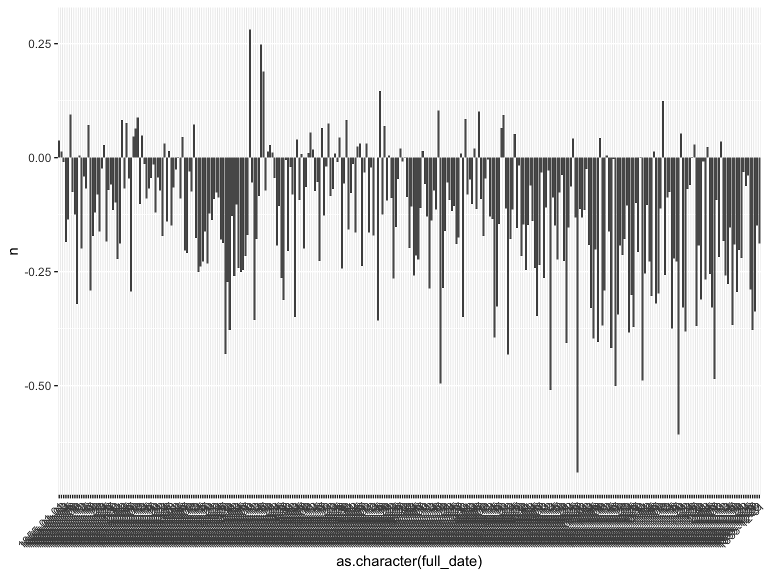
Figure 13.1: Sentiment Over Time