11 Term Frequencies
The first thing you might want to do with a large dataset of text is to count the words within it. Doing this with newspaper data can be particularly significant, because it’s quite easy to discover trends, reporting practices, and particular events. By count words, and sorting by date, or by title, it’s possible to make some interesting comparisons and conclusions in the makeup of different titles, or to understand changes in reporting over time. Again, as this is a small sample, the conclusions will be light, but the aim is the show the method.
11.1 Load the news dataframe and relevant libraries
The first thing is to take the newss dataframe, as made in the previous chapter, and load it into memory, if it isn’t already.
load('news_sample_dataframe')The two libraries we’ll use are tidyverse, as usual, and tidytext. The dataframe we created has a row per article. This is a really easy format to do text mining with, using the techniques from here: https://www.tidytextmining.com/, and the library tidytext. If it’s not installed, use ```install.packages(‘tidytext’) to install it.
library(tidyverse)
library(tidytext)
library(lubridate)
Take a quick look at the dataframe:
glimpse(news_sample_dataframe)## Rows: 83,656
## Columns: 7
## $ article_code <int> 1, 2, 3, 4, 5, 6, 7, 8, 9, 10, 11, 12, 13, 14, 15, 16, 17…
## $ art <chr> "0001", "0002", "0003", "0004", "0005", "0006", "0007", "…
## $ text <chr> "esP e STYLE=superscript allall J STYLE=superscript o…
## $ title <chr> "", "", "", "", "", "", "", "", "", "", "", "", "", "", "…
## $ year <chr> "1855", "1855", "1855", "1855", "1855", "1855", "1855", "…
## $ date <chr> "0619", "0619", "0619", "0619", "0619", "0619", "0619", "…
## $ full_date <date> 1855-06-19, 1855-06-19, 1855-06-19, 1855-06-19, 1855-06-…11.2 Tokenise the text using unnest_tokens()
Most analysis involves tokenising the text. This divides the text into ‘tokens’ - representing one unit. A unit is often a word, but could be a bigram - a sequence of two consecutive words, or a trigram, a sequence of three consecutive words. With the library tidytext, this is done using a function called unnest_tokens(). This will split the column containing the text of the article into a long dataframe, with one word per row.
The two most important arguments to ``unnest_tokensareoutputandinput```. This is fairly self explanatory. Just pass it the name you would like to give the new column of words (or n-grams) and the column you’d like to split up: in this case the original column is called ‘text’, and we’d like our column of words to be called words.
news_sample_dataframe %>%
  unnest_tokens(output = word, input = text) %>% head(10)
## # A tibble: 10 × 7
## article_code art title year date full_date word
## <int> <chr> <chr> <chr> <chr> <date> <chr>
## 1 1 0001 "" 1855 0619 1855-06-19 esp
## 2 1 0001 "" 1855 0619 1855-06-19 e
## 3 1 0001 "" 1855 0619 1855-06-19 style
## 4 1 0001 "" 1855 0619 1855-06-19 superscript
## 5 1 0001 "" 1855 0619 1855-06-19 allall
## 6 1 0001 "" 1855 0619 1855-06-19 j
## 7 1 0001 "" 1855 0619 1855-06-19 style
## 8 1 0001 "" 1855 0619 1855-06-19 superscript
## 9 1 0001 "" 1855 0619 1855-06-19 o
## 10 1 0001 "" 1855 0619 1855-06-19 poYou can also specify an argument for token, allowing you to split the text into sentences, characters, lines, or n-grams.If you split into n-grams, you need to use the argument n= to specify how many consecutive words you’d like to use.
Like this:
news_sample_dataframe %>%
  unnest_tokens(output = word,
                input = text,
                token = 'ngrams',
                n =3)
## # A tibble: 59,001,206 × 7
## article_code art title year date full_date word
## <int> <chr> <chr> <chr> <chr> <date> <chr>
## 1 1 0001 "" 1855 0619 1855-06-19 esp e style
## 2 1 0001 "" 1855 0619 1855-06-19 e style superscript
## 3 1 0001 "" 1855 0619 1855-06-19 style superscript allall
## 4 1 0001 "" 1855 0619 1855-06-19 superscript allall j
## 5 1 0001 "" 1855 0619 1855-06-19 allall j style
## 6 1 0001 "" 1855 0619 1855-06-19 j style superscript
## 7 1 0001 "" 1855 0619 1855-06-19 style superscript o
## 8 1 0001 "" 1855 0619 1855-06-19 superscript o po
## 9 1 0001 "" 1855 0619 1855-06-19 o po 34
## 10 1 0001 "" 1855 0619 1855-06-19 po 34 d
## # … with 59,001,196 more rows11.3 Pre-process to clean and remove stop words
Before we do any counting, there’s a couple more processing steps. I’m going to remove ‘stop words’. Stop words are very frequently-used words which often crowd out more interesting results. This isn’t always the case, and you shoudln’t just automatically get rid of them, but rather think about what it is yo uare looking for. For this tutorial, though, the results will be more interesting if it’s not just a bunch of ‘the’ and ‘at’ and so forth.
This is really easy. We load a dataframe of stopwords, which is included in the tidytext package.
data("stop_words")Next use the function anti_join(). This bascially removes any word in our word list which is also in the stop words list
news_sample_dataframe %>%
  unnest_tokens(output = word, input = text) %>%
  anti_join(stop_words)
## Joining, by = "word"## # A tibble: 30,577,829 × 7
## article_code art title year date full_date word
## <int> <chr> <chr> <chr> <chr> <date> <chr>
## 1 1 0001 "" 1855 0619 1855-06-19 esp
## 2 1 0001 "" 1855 0619 1855-06-19 style
## 3 1 0001 "" 1855 0619 1855-06-19 superscript
## 4 1 0001 "" 1855 0619 1855-06-19 allall
## 5 1 0001 "" 1855 0619 1855-06-19 style
## 6 1 0001 "" 1855 0619 1855-06-19 superscript
## 7 1 0001 "" 1855 0619 1855-06-19 po
## 8 1 0001 "" 1855 0619 1855-06-19 34
## 9 1 0001 "" 1855 0619 1855-06-19 style
## 10 1 0001 "" 1855 0619 1855-06-19 superscript
## # … with 30,577,819 more rowsA couple of words from the .xml have managed to sneak through our text processing: ‘style’ and ‘superscript’. I’m also going to remove these, plus a few more common OCR errors for the word ‘the’.
I’m also going to remove any word with two or less characters, and any numbers. Again, these are optional steps.
I’ll store the dataframe as a variable called ‘tokenised_news_sample’. I’ll also save it using save(), which turns it into an .rdata file, which can be used later.
11.4 Create and save a dataset of tokenised text
tokenised_news_sample = news_sample_dataframe %>%
  unnest_tokens(output = word, input = text) %>%
  anti_join(stop_words) %>%
  filter(!word %in% c('superscript',
                      'style',
                      'de',
                      'thle',
                      'tile',
                      'tie',
                      'tire',
                      'tiie',
                      'tue',
                      'amp')) %>%
  filter(!str_detect(word, '[0-9]{1,}')) %>%
  filter(nchar(word) > 2)
## Joining, by = "word"save(tokenised_news_sample, file = 'tokenised_news_sample')11.5 Count the tokens
Now I can use all the tidyverse commands like filter, count, tally and so forth on the data, making it really easy to do basic analysis like word frequency counting. It’s a large list of words (about 23 million), so these processes might take a few seconds, even on a fast computer.
A couple of examples:
11.5.1 The top words overall:
tokenised_news_sample %>%
  group_by(word) %>%
  tally() %>%
  arrange(desc(n)) %>% head(20)
## # A tibble: 20 × 2
## word n
## <chr> <int>
## 1 day 70802
## 2 lord 66234
## 3 london 59544
## 4 street 58403
## 5 time 57188
## 6 house 49212
## 7 war 48262
## 8 sad 47300
## 9 sir 45300
## 10 government 43278
## 11 cent 40611
## 12 royal 40040
## 13 john 38177
## 14 public 34011
## 15 captain 32784
## 16 country 32677
## 17 liverpool 32246
## 18 army 32049
## 19 received 29738
## 20 french 2926711.5.2 The top five words for each day in the dataset:
tokenised_news_sample %>%
  group_by(full_date, word) %>%
  tally() %>%
  arrange(full_date, desc(n)) %>%
  group_by(full_date) %>%
  top_n(5) %>% head(100)
## Selecting by n## # A tibble: 100 × 3
## # Groups: full_date [20]
## full_date word n
## <date> <chr> <int>
## 1 1855-01-01 day 197
## 2 1855-01-01 royal 135
## 3 1855-01-01 london 132
## 4 1855-01-01 lord 122
## 5 1855-01-01 steam 120
## 6 1855-01-02 cent 226
## 7 1855-01-02 day 219
## 8 1855-01-02 london 197
## 9 1855-01-02 time 145
## 10 1855-01-02 royal 131
## # … with 90 more rows11.5.3 Check the top words per title (well, variant titles in this case):
tokenised_news_sample %>%
  group_by(title, word) %>%
  tally() %>%
  arrange(desc(n)) %>%
  group_by(title) %>%
  top_n(5)
## Selecting by n## # A tibble: 5 × 3
## # Groups: title [1]
## title word n
## <chr> <chr> <int>
## 1 "" day 70802
## 2 "" lord 66234
## 3 "" london 59544
## 4 "" street 58403
## 5 "" time 57188You can also summarise by units of time, using the function cut(). This rounds the date down to the nearest day, year or month. Once it’s been rounded down, we can count by this new value.
11.5.4 Top words by month
tokenised_news_sample %>%
  mutate(month = cut(full_date, 'month')) %>%
  group_by(month, word) %>%
  tally() %>%
  arrange(month, desc(n)) %>%
  group_by(month) %>%
  top_n(5)
## Selecting by n## # A tibble: 60 × 3
## # Groups: month [12]
## month word n
## <fct> <chr> <int>
## 1 1855-01-01 jan 7162
## 2 1855-01-01 day 5462
## 3 1855-01-01 london 4615
## 4 1855-01-01 war 4584
## 5 1855-01-01 time 4272
## 6 1855-02-01 lord 7832
## 7 1855-02-01 feb 5710
## 8 1855-02-01 government 4904
## 9 1855-02-01 house 4879
## 10 1855-02-01 day 4650
## # … with 50 more rows11.6 Visualise the Results
We can also pipe everything directly to a plot. ‘Ship’ is a common word: did its use change over the year? Here we use filter() to filter out everything except the word (or words) we’re interested in.
For this to be in any way meaningful, you should think of some way of normalising the results, so that the number is of a percentage of the total words in that title, for example. The raw numbers may just indicate a change in the total volume of text.
11.6.1 Words over time
tokenised_news_sample %>%
  filter(word == 'ship') %>%
    mutate(week = ymd(cut(full_date, 'week'))) %>%
  group_by(week, word) %>%
  tally() %>% ggplot() + geom_col(aes(x = week, y = n))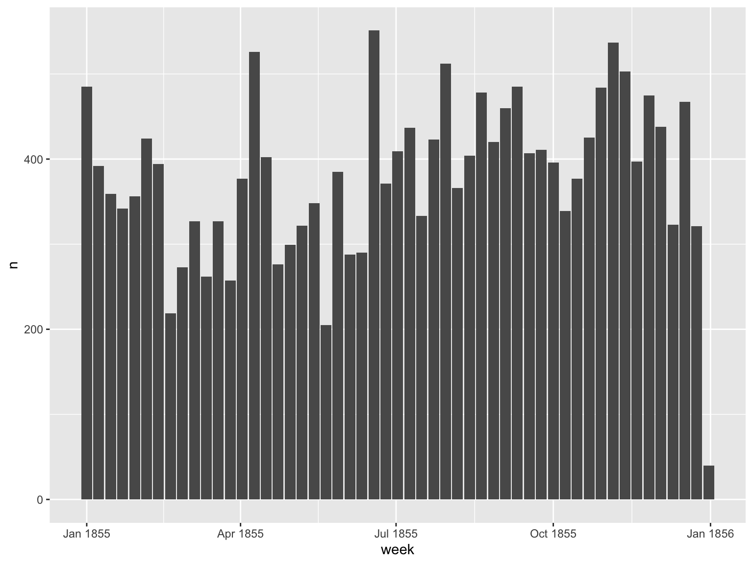
Figure 11.1: Chart of the Word ‘ship’ over time
11.6.2 Chart several words over time
Charting a couple of words might be more interesting: How about ‘steam’ versus ‘sail’?
tokenised_news_sample %>%
  filter(word %in% c('steam', 'sail')) %>%
    mutate(week = ymd(cut(full_date, 'week')))%>%
  group_by(week, word) %>%
  tally() %>% ggplot() +
  geom_line(aes(x = week, y = n, color = word))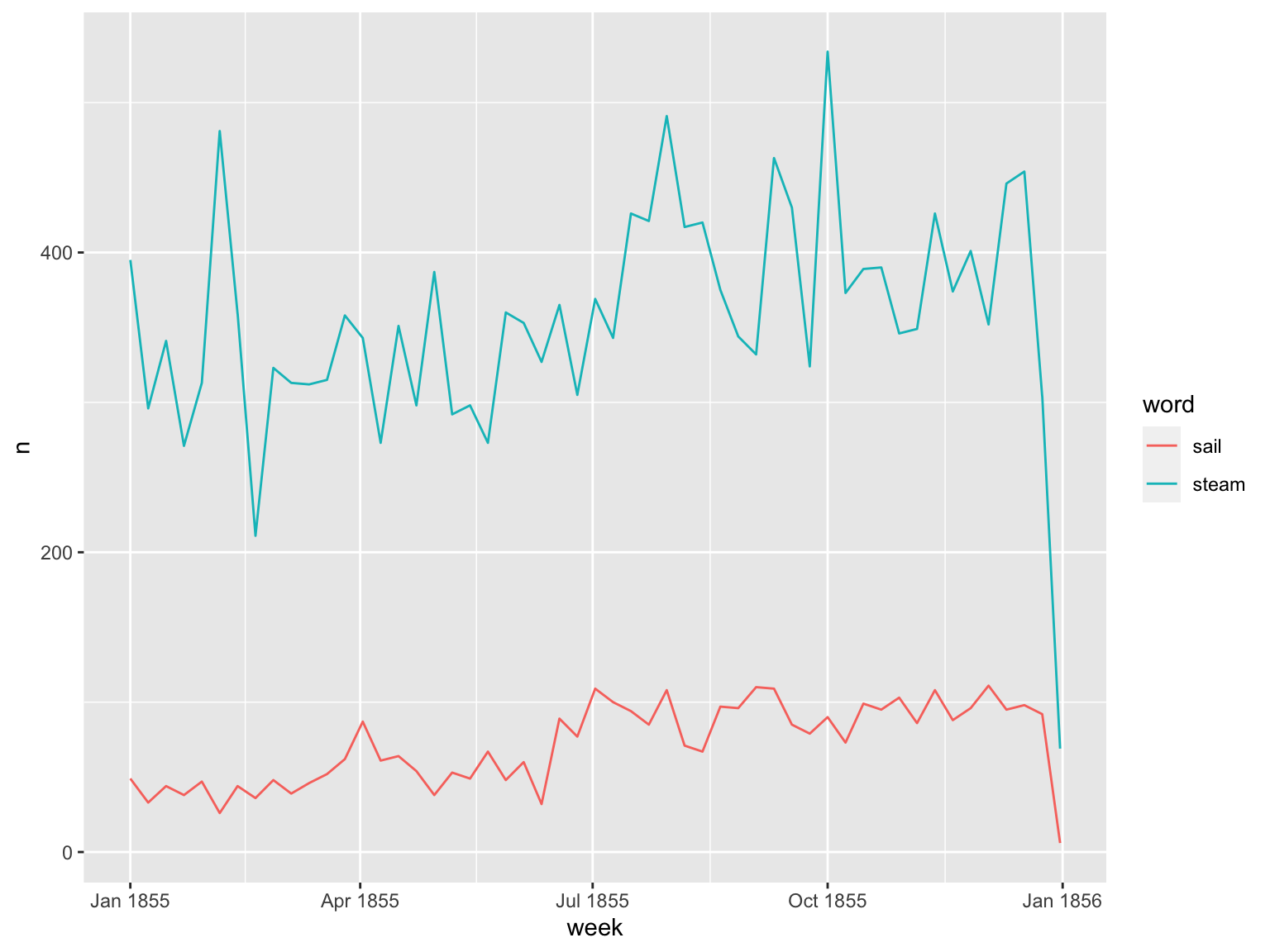
Figure 11.2: Charting Several Words Over the Entire Dataset
11.7 Interactive Shiny Application
If you’d like to explore some of the text frequencies as extracted in this chapter, I’ve created an application to do so without going through any of the code on the page:
11.8 Further reading
The best place to learn more is by reading the ‘Tidy Text Mining’ book available at https://www.tidytextmining.com. This book covers a whole range of text mining topics, including those used in the next few chapters.