Chapter 9 Meauring Volatility

9.1 Imagine this

• Your company owns several facilities for the manufacture and distribution of polysyllabic acid, a compound used in several industries (and of course quite fictional!).
• Inputs to the manufacturing and distribution processes include various petroleum products and natural gas. Price swings can be quite volatile, and you know that Brent crude exhibits volatility clustering.
• Working capital management is always a challenge, and recent movements in the dollar against the euro and pound sterling have impacted cash conversion severely.
• Your CFO, with a memory of having worked at Metallgesellschaft in the 1990’s, is being pushed by the board to hedge the input price risk using futures and over-the-counter (OTC) instruments.

The board is concerned because the company has missed its earnings estimate for the fifth straight quarter in a row. Shareholders are not pleased. The culprits seem to be a volatile cost of goods sold coupled with large swings in some revenue segments in the United Kingdom (UK) and the European Union (EU).Your CFO has handed you the job of organizing the company’s efforts to understand the limits your exposure can extend. The analysis will be used to develop policy guidelines for managing customer and vendor relationships.

9.1.1 Example

1. What are the key business questions you should ask about energy pricing patterns?
2. What systematic approach might you use to manage input volatility?

Here are some ideas.

1. Key business questions might be

• Which input prices and exchange rates are more volatile than others and when?
• Are price movements correlated?
• In times of market stress how volatile can they be?
• Are there hedging instruments we can deploy or third parties we can use to mitigate pricing risk?

2. Managing volatility

• Set up an input monitoring system to know what inputs affect what components and costs of running the manufacturing and distribution processes.
• Monitor price movements and characteristics and measure severity of impact on key operating income components by process.
• Build in early warning indicators of intolerable swings in prices.
• Build a playbook to manage the otherwise insurgent and unanticipated retained risk of input price volatility in manufacturing and distribution processes.

Topics we got to in previous chapters:

• Explored stylized fact of financial market data
• Learned just how insidious volatility really is
• Acquired new tools like acf, pacf, ccf to explore time series
• Analyzed market, credit, and operational risk

In this chapter we will

• Remember the stylized facts and use a fix for volatility clustering
• Fit AR-GARCH models
• Simulate volatility from the AR-GARCH model
• Measure the risks of various exposures

9.2 What is All the Fuss About?

We have already looked at volatility clustering. ARCH models are one way to model this phenomenon.

ARCH stands for

• Autoregressive (lags in volatility)
• Conditional (any new values depend on others)
• Heteroscedasticity (Greek for varying volatility, here time-varying)

These models are especially useful for financial time series that exhibit periods of large return movements alongside intermittent periods of relative calm price changes.

An experiment is definitely in order.

The AR+ARCH model can be specified starting with \(z(t)\) standard normal variables and initial (we will overwrite this in the simulation) volatility series \(\sigma(t)^2 = z(t)^2\). We then condition these variates with the square of their variances \(\varepsilon(t) = (sigma^2)^{1/2} z(t)\). Then we first compute for each date \(t = 1 ... n\),

\[ \varepsilon(t) = (sigma^2)^{1/2} z(t) \]

Then, using this conditional error term we compute the autoregression (with lag 1 and centered at the mean \(\mu\))

\[ y(t) = \mu + \phi(y(t-1) - \mu) + \varepsilon(t) \]

Now we are ready to compute the new variance term.

n <-  10500 ## lots of trials
z <- rnorm(n) ## sample standard normal distribution variates
e <-  z ## store variates
y <-  z ## store again in a different place
sig2 <-  z^2 ## create volatility series
omega <-  1 ## base variance
alpha <-  0.55 ## Markov dependence on previous variance
phi <-  0.8 ## mMarkov dependence on previous period
mu <-  0.1 ## average return
omega/(1-alpha) ; sqrt(omega/(1-alpha))

## [1] 2.222222

## [1] 1.490712

set.seed("1012")
for (t in 2:n) ## Because of lag start at second date
{
  e[t] <- sqrt(sig2[t])*z[t]          ## 1. e is conditional on sig
  y[t] <-  mu + phi*(y[t-1]-mu) + e[t] ## 2. generate returns
  sig2[t+1] <-  omega + alpha * e[t]^2 ## 3. generate new sigma^2 to feed 1.
}

A plot is a little than instructive.

par(mfrow = c(2, 4))
plot(z[10001:n], type = "l", xlab = "t", 
    ylab = expression(epsilon), main = "1. Simple noise")
plot(sqrt(sig2[10000:n]), type = "l", 
    xlab = "t", ylab = expression(sigma[t]), 
    main = "2. Conditional sigma")
plot(e[10001:n], type = "l", xlab = "t", 
    ylab = "a", main = "3. ARCH")
plot(y[10001:n], type = "l", xlab = "t", 
    ylab = "y", main = "4. AR+ARCH")
acf(e[10001:n], main = "5. ARCH")
acf(abs(e[10001:n]), main = "6. Absolute ARCH value")
acf(y[10001:n], main = "7. AR+ARCH")
acf(abs(y[10001:n]), main = "8. Absolute AR+ARCH value")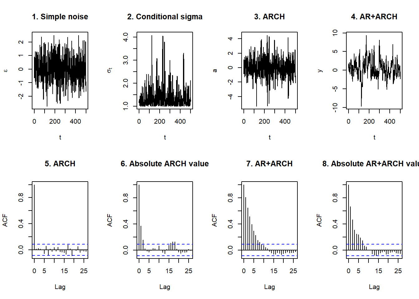

## 

What do we see?

1. Large outlying peaks in the conditional standard deviation
2. Showing up as well in the ARCH plot
3. AR adds the clustering as returns attempt to revert to the long run mean of \(\mu =\) 10%.
4. Patterns reminiscent of clustering occur with thick and numerous lags in the acf plots. There is persistence of large movements both up and down.

Why does it matter?

• Revenue received from customer contracts priced with volatility clustering will act like the prices: when in a downward spiral, that spiral will amplify more than when prices try to trend upward.
• The same will happen with the value of inventory and the costs of inputs.
• All of this adds up to volatile EBITDA (Earnings Before Interest and Tax adding in non-cash Depreciation and Amortization), missed earnings targets, shareholders selling, the stock price dropping, and equity-based compensation falling.

9.3 Lock and Load…

We have more than one way to estimate the parameters of the AR-ARCH process. Essentially we are running yet another “regression.” Let’s first load some data to tackle the CFO’s questions around exposures in the UK, EU, and in the oil market.

require(rugarch)
require(qrmdata)
require(xts)
## The exchange rate data was obtained
## from OANDA (http://www.oanda.com/)
## on 2016-01-03
data("EUR_USD")
data("GBP_USD")
## The Brent data was obtained from
## Federal Reserve Economic Data
## (FRED) via Quandl on 2016-01-03
data("OIL_Brent")
data.1 <- na.omit(merge(EUR_USD, GBP_USD, 
    OIL_Brent))
P <- data.1
R <- na.omit(diff(log(P)) * 100)
names.R <- c("EUR.USD", "GBP.USD", "OIL.Brent")
colnames(R) <- names.R
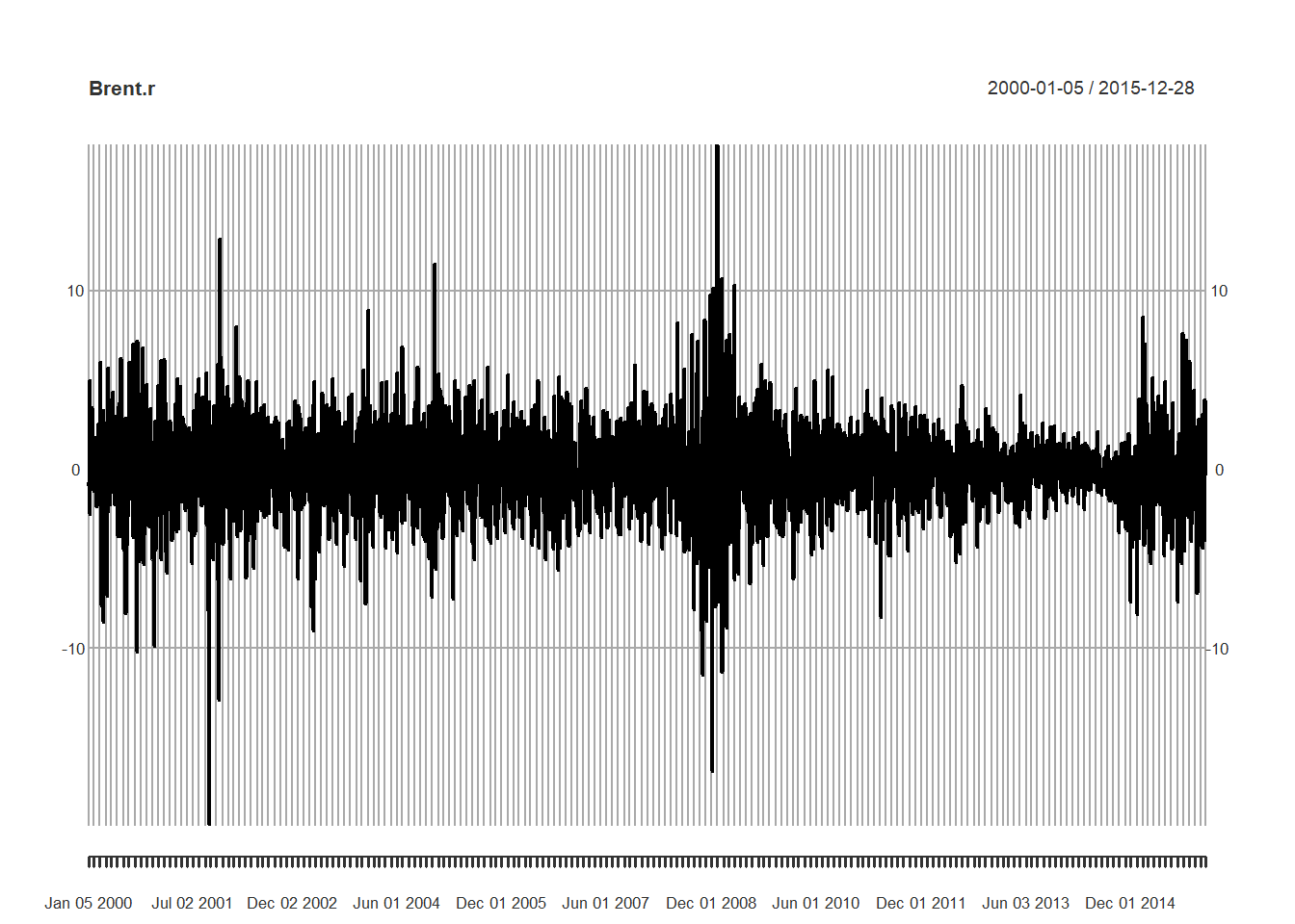
Brent.p <- data.1[, 3]
Brent.r <- R[, 3]  ## Pull out just the Brent pieces

Then we plot the data, transformations, and autocorrelations.

## 
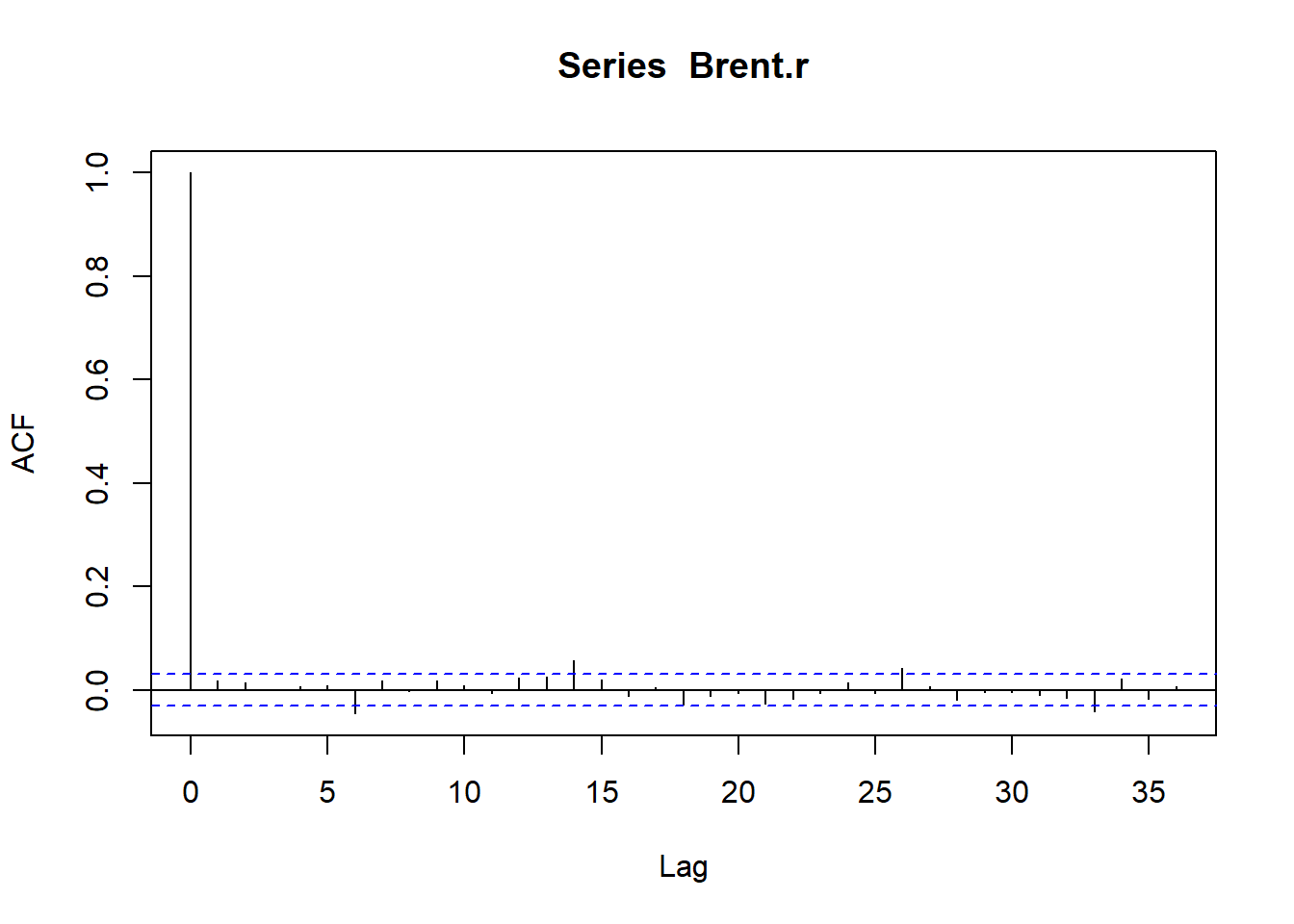
##  Box-Ljung test
## 
## data:  Brent.r
## X-squared = 32.272, df = 14, p-value = 0.003664

The p-value is small enough to more than reject the null hypothesis that the 14-day lag is not significantly different from zero.

9.4 It is Fitting…

Our first mechanical task is to specify the ARMA-GARCH model. First we specify.

1. Use the ugarchspec function to specify a plain vanilla sGarch model.
2. garchOrder = c(1,1) means we are using the first lags of residuals squared and variance or (with \(\omega\), “omega,” the average variance, \(\sigma_t^2\)), here of Brent returns): \[ \sigma_t^2 = \omega + \alpha_1 \varepsilon_{t-1}^2 + \beta_{t-1} \sigma_{t-1}^2. \]
3. Use armaOrder = c(1,0) to specify the mean Brent return model with long run average \(\mu\) \[ r_t = \mu + \psi_1 y_{t-1} + \psi_2 \varepsilon_{t-1}. \]
4. Include means as in the equations above.
5. Specify the distribution as norm for normally distributed innovations \(\varepsilon_t\). We will also compare this fit with the std Student’s t-distribution innovations using the Akaike Information Criterion (AIC).
6. Fit the data to the model using ugarchfit.

AR.GARCH.Brent.Norm.spec <- ugarchspec(variance.model = list(model = "sGARCH", 
    garchOrder = c(1, 1)), mean.model = list(armaOrder = c(1, 
    0), include.mean = TRUE), distribution.model = "norm")
fit.Brent.norm <- ugarchfit(spec = AR.GARCH.Brent.Norm.spec, 
    data = Brent.r)

Let’s look at the conditional quantiles from this model, otherwise known as the VaR limits, nominally set at 99%.

## First the series with conditional
## quantiles
plot(fit.Brent.norm, which = 2)

We might think about hedging the very highs and very lows.

## 
## please wait...calculating quantiles...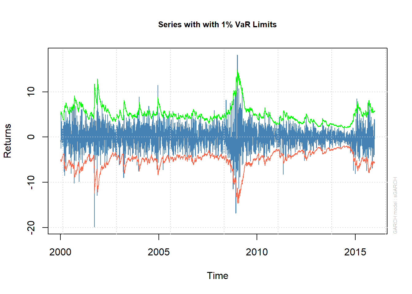

Now let’s generate a panel of plots.

par(mfrow = c(2, 2))
## acf of absolute data - shows serial
## correlation
plot(fit.Brent.norm, which = 6)
## QQplot of data - shows
## leptokurtosis of standardized
## rediduals - normal assumption not
## supported
plot(fit.Brent.norm, which = 9)
## acf of standardized residuals -
## shows AR dynamics do a reasonable
## job of explaining conditional mean
plot(fit.Brent.norm, which = 10)
## acf of squared standardized
## residuals - shows GARCH dynamics do
## a reasonable job of explaining
## conditional sd
plot(fit.Brent.norm, which = 11)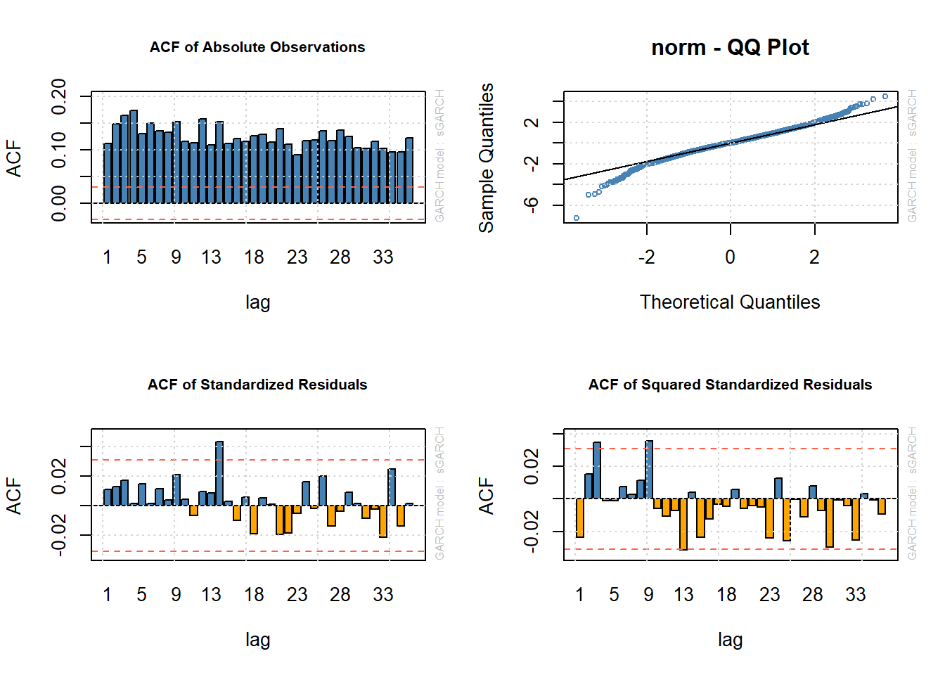

par(mfrow = c(1, 1))

9.4.1 Example

Let’s redo the GARCH estimation, now using the possibly more realistic thicker tails of the Student’s t-distribution for the \(\varepsilon\) innovations. Here we just replace norm with std in the distribution.model = statement in the ugarchspec function.

## Fit an AR(1)-GARCH(1,1) model with
## student innovations
AR.GARCH.Brent.T.spec <- ugarchspec(variance.model = list(model = "sGARCH", 
    garchOrder = c(1, 1)), mean.model = list(armaOrder = c(1, 
    0), include.mean = TRUE), distribution.model = "std")
fit.Brent.t <- ugarchfit(spec = AR.GARCH.Brent.T.spec, 
    data = Brent.r)
par(mfrow = c(2, 2))
plot(fit.Brent.t, which = 6)
plot(fit.Brent.t, which = 9)
plot(fit.Brent.t, which = 10)
plot(fit.Brent.t, which = 11)
par(mfrow = c(1, 1))

Here are some results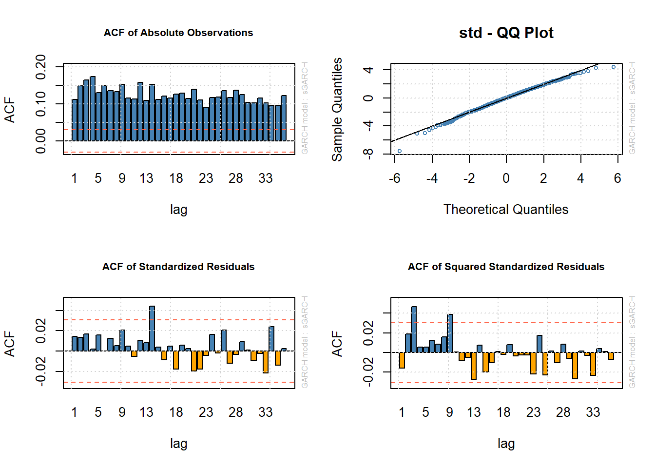

1. ACF of absolute observations indicates much volatility clustering.
2. These are significantly dampened by the AR-ARCH estimation with almost bounded standardized residuals (residual / standard error).
3. More evidence of this comes from the ACF of the squared standardized residuals.
4. It appears that this AR-GARCH specification and Student’s t-distributed innovations captures most of the movement in volatility for Brent.

Which model? - Use the Akaike Information Criterion (AIC) to measure information leakage from a model. - AIC measures the mount of information used in a model specified by a log likelihood function. - Likelihood: probability that you will observe the Brent returns given the parameters estimated by (in this case) the GARCH(1,1) model with normal or t-distributed innovations. - Smallest information leakage (smallest AIC) is the model for us.

Compute 5. Using normally distributed innovations produces a model with AIC = 4.2471. 6. Using Student’s t-distributed innovations produces a model with AIC = 4.2062. 7. GARCH(1,1) with Student’s t-distributed innovations is more likely to have less information leakage than the GARCH(1,1) with normally distributed innovations.

Here are some common results we can pull from the fit model:

coef(fit.Brent.t)

##         mu        ar1      omega     alpha1      beta1      shape 
## 0.04018002 0.01727725 0.01087721 0.03816097 0.96074399 7.03778415

Coefficients include:

• mu is the long run average Brent return.
• ar1 is the impact of one day lagged return on today’s return.
• omega is the long run variance of Brent return.
• alpha1 is the impact of lagged squared variance on today’s return.
• beta1 is the impact of lagged squared residuals on today’s Brent return.
• shape is the degrees of freedom of the Student’s t-distribution and the bigger this is, the thicker the tail.

Let’s plot the star of this show: time-varying volatility.

coef(fit.Brent.t)

##         mu        ar1      omega     alpha1      beta1      shape 
## 0.04018002 0.01727725 0.01087721 0.03816097 0.96074399 7.03778415

plot(sigma(fit.Brent.t))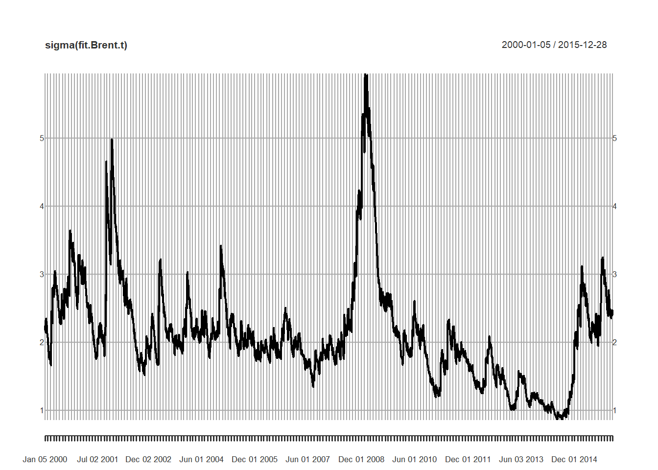

Here’s the other reason for going through this exercise: we can look at any Brent volatility range we like.

plot(quantile(fit.Brent.t, 0.99))

Next we plot and test the residuals:

z.hat <- residuals(fit.Brent.t, standardize = TRUE)
plot(z.hat)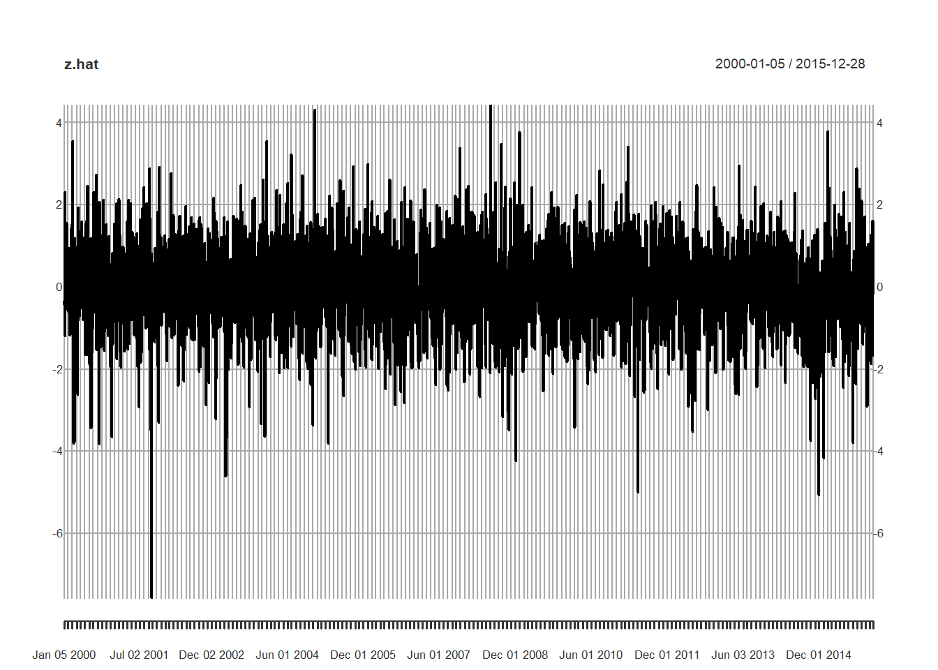

hist(z.hat)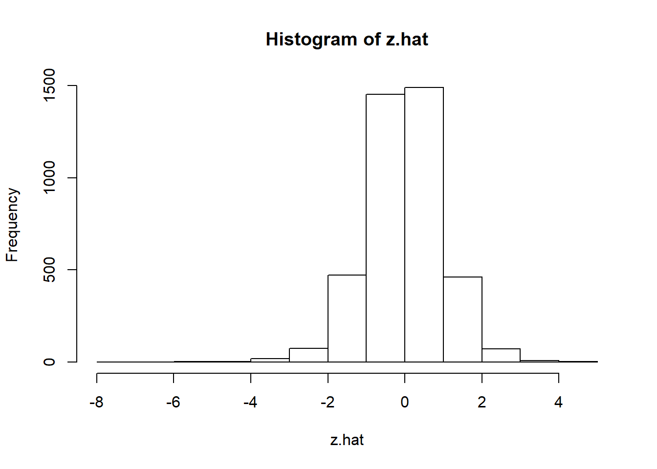

mean(z.hat)

## [1] -0.0181139

var(z.hat)

##          [,1]
## [1,] 1.000682

require(moments)
skewness(z.hat)

## [1] -0.3207327
## attr(,"method")
## [1] "moment"

kurtosis(z.hat)

## [1] 2.048561
## attr(,"method")
## [1] "excess"

shapiro.test(as.numeric(z.hat))

## 
##  Shapiro-Wilk normality test
## 
## data:  as.numeric(z.hat)
## W = 0.98439, p-value < 2.2e-16

jarque.test(as.numeric(z.hat))

## 
##  Jarque-Bera Normality Test
## 
## data:  as.numeric(z.hat)
## JB = 780.73, p-value < 2.2e-16
## alternative hypothesis: greater

What do we see?

• Left skewed.
• Thick tailed.
• Potentially large losses can occur with ever larger losses in the offing.
• More negative than positive.
• Both standard tests indicate rejection of the null hypothesis that the series is normally distributed.

9.5 Simulate… again until Morale Improves…

1. Specify the AR-GARCH process using the parameters from the fit.Brent.t results.
2. Generate 2000 paths.

require(rugarch)
GARCHspec <- ugarchspec(variance.model = list(model = "sGARCH", 
    garchOrder = c(1, 1)), mean.model = list(armaOrder = c(1, 
    0), include.mean = TRUE), distribution.model = "std", 
    fixed.pars = list(mu = 0.04, ar1 = 0.0173, 
        omega = 0.0109, alpha1 = 0.0382, 
        beta1 = 0.9607, shape = 7.0377))
GARCHspec

## 
## *---------------------------------*
## *       GARCH Model Spec          *
## *---------------------------------*
## 
## Conditional Variance Dynamics    
## ------------------------------------
## GARCH Model      : sGARCH(1,1)
## Variance Targeting   : FALSE 
## 
## Conditional Mean Dynamics
## ------------------------------------
## Mean Model       : ARFIMA(1,0,0)
## Include Mean     : TRUE 
## GARCH-in-Mean        : FALSE 
## 
## Conditional Distribution
## ------------------------------------
## Distribution :  std 
## Includes Skew    :  FALSE 
## Includes Shape   :  TRUE 
## Includes Lambda  :  FALSE

## Generate two realizations of length
## 2000
path <- ugarchpath(GARCHspec, n.sim = 2000, 
    n.start = 50, m.sim = 2)

There is a special plotting function for “uGARCHpath” objects.

plot(path, which = 1)
plot(path, which = 2)
plot(path, which = 3)
plot(path, which = 4)
## How to see the documentation of the
## plot function showMethods('plot')
## getMethod('plot',c(x='GPDTAILS',
## y='missing'))

There is also an extraction function for the volatility.

vol <- sigma(path)
head(vol)

##         [,1]     [,2]
## T+1 2.950497 5.018346
## T+2 2.893878 4.927087
## T+3 2.848404 4.849797
## T+4 2.802098 4.819258
## T+5 2.880778 4.768916
## T+6 2.826746 4.675612

plot(vol[, 1], type = "h")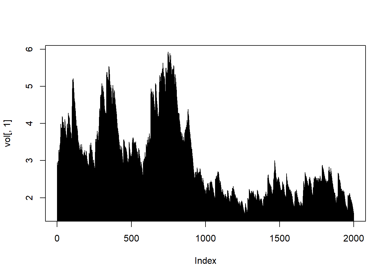

plot(vol[, 2], type = "h")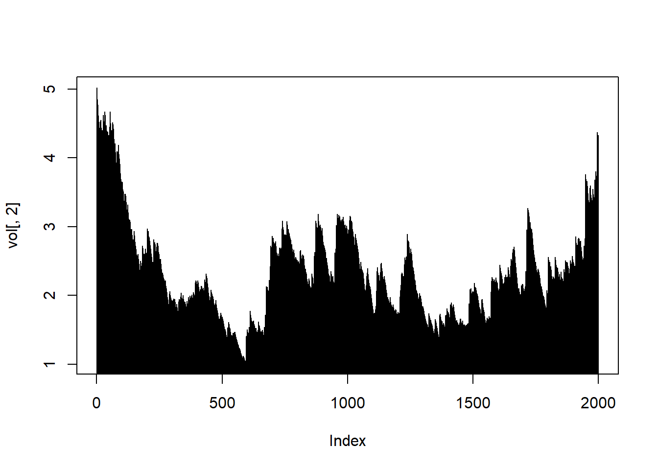

Here is a little more background on the classes used.

series <- path@path
## series is a simple list
class(series)

## [1] "list"

names(series)

## [1] "sigmaSim"  "seriesSim" "residSim"

## the actual simulated data are in
## the matrix/vector called
## 'seriesSim'
X <- series$seriesSim
head(X)

##            [,1]       [,2]
## [1,]  0.1509418  1.4608335
## [2,]  1.2644849 -2.1509425
## [3,] -1.0397785  4.0248510
## [4,]  4.4369130  3.4214660
## [5,] -0.3076812 -0.1104726
## [6,]  0.4798977  2.7440751

9.5.1 Example

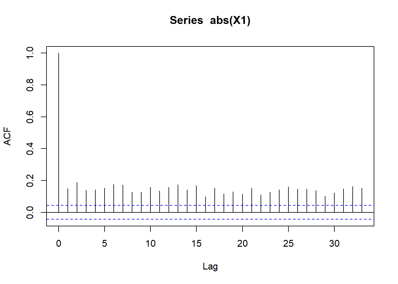
Does the simulated series conform to stylized facts?

X1 <- X[, 1]
acf(X1)
acf(abs(X1))
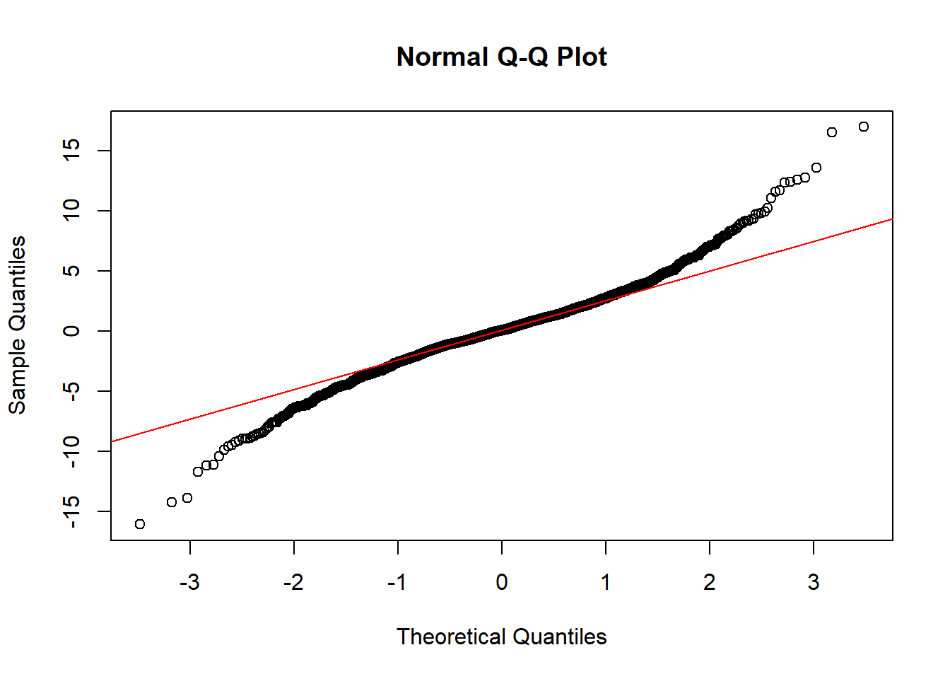
qqnorm(X1)
qqline(X1, col = 2)
shapiro.test(X1)

Remember the stylized facts?

1. Volatility clustering.
2. If it’s bad, it gets worse more often.
3. If it’s good, it get better less often.
4. High stress means high volatility.

Here are some results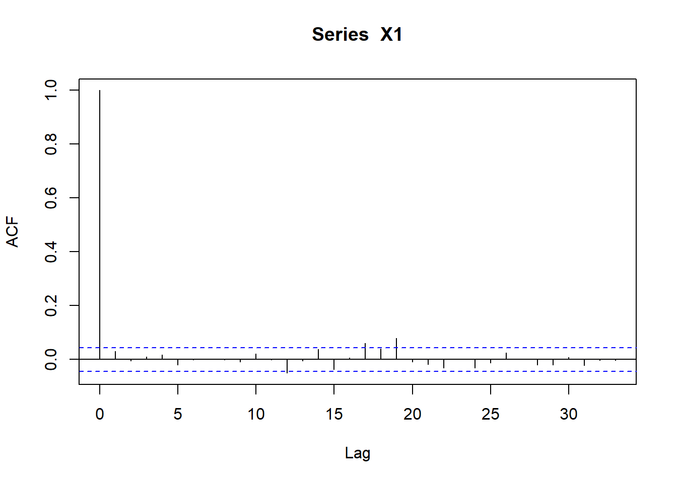

## 
##  Shapiro-Wilk normality test
## 
## data:  X1
## W = 0.97164, p-value < 2.2e-16

Shapiro-Wilk test - Null hypothesis: normally distributed. - Reject null if p-value is small enough. - Must verify with a QQ plot of empirical versus theoretical quantiles.

The stylized facts perdure.

9.6 Now for Something Really Interesting

We go from univariate GARCH to multivariate GARCH…and use the most recent technique to make it into the fray:

• The Dynamic Conditional Correlation of Nobel Laureate Robert Engle.
• In the GARCH model we just did, individual assets follow their own univariate GARCH process: they now have time-varying volatilities.
• Engle figured out how to make the correlations among asset return also time-varying.

Why? - What if we have a portfolio, like the accounts receivable that might face variations in exchange rates and in Brent oil. - We would need to know the joint volatilities and dependences of these three factors as they contribute to overall accounts receivable volatility. - We would use these conditional variances at least to model option prices on instruments to manage currency and commodity risk.

require(rmgarch)
garch11.spec <- ugarchspec(mean.model = list(armaOrder = c(0, 
    0)), variance.model = list(garchOrder = c(1, 
    1), model = "sGARCH"), distribution.model = "std")
dcc.garch11.spec = dccspec(uspec = multispec(replicate(3, 
    garch11.spec)), dccOrder = c(1, 1), 
    distribution = "mvt")

Look at dcc.garch11.spec

dcc.garch11.spec

## 
## *------------------------------*
## *       DCC GARCH Spec         *
## *------------------------------*
## Model          :  DCC(1,1)
## Estimation     :  2-step
## Distribution   :  mvt
## No. Parameters :  21
## No. Series     :  3

Now for the fit (takes more than 27.39 seconds on my laptop…)

dcc.fit <- dccfit(dcc.garch11.spec, data = R)

Now let’s get some results:

## 
## *---------------------------------*
## *          DCC GARCH Fit          *
## *---------------------------------*
## 
## Distribution         :  mvt
## Model                :  DCC(1,1)
## No. Parameters       :  21
## [VAR GARCH DCC UncQ] : [0+15+3+3]
## No. Series           :  3
## No. Obs.             :  4057
## Log-Likelihood       :  -12820.82
## Av.Log-Likelihood    :  -3.16 
## 
## Optimal Parameters
## -----------------------------------
##                     Estimate  Std. Error    t value Pr(>|t|)
## [EUR.USD].mu        0.006996    0.007195    0.97238 0.330861
## [EUR.USD].omega     0.000540    0.000288    1.87540 0.060738
## [EUR.USD].alpha1    0.036643    0.001590   23.04978 0.000000
## [EUR.USD].beta1     0.962357    0.000397 2426.49736 0.000000
## [EUR.USD].shape     9.344066    1.192132    7.83811 0.000000
## [GBP.USD].mu        0.006424    0.006386    1.00594 0.314447
## [GBP.USD].omega     0.000873    0.000327    2.67334 0.007510
## [GBP.USD].alpha1    0.038292    0.002217   17.27004 0.000000
## [GBP.USD].beta1     0.958481    0.000555 1727.86868 0.000000
## [GBP.USD].shape    10.481272    1.534457    6.83061 0.000000
## [OIL.Brent].mu      0.040479    0.026696    1.51627 0.129450
## [OIL.Brent].omega   0.010779    0.004342    2.48228 0.013055
## [OIL.Brent].alpha1  0.037986    0.001941   19.57467 0.000000
## [OIL.Brent].beta1   0.960927    0.000454 2118.80489 0.000000
## [OIL.Brent].shape   7.040287    0.729837    9.64639 0.000000
## [Joint]dcca1        0.009915    0.002821    3.51469 0.000440
## [Joint]dccb1        0.987616    0.004386  225.15202 0.000000
## [Joint]mshape       9.732509    0.652707   14.91100 0.000000
## 
## Information Criteria
## ---------------------
##                    
## Akaike       6.3307
## Bayes        6.3633
## Shibata      6.3306
## Hannan-Quinn 6.3423
## 
## 
## Elapsed time : 11.89964

• The mean models of each series (EUR.USD, GPB.USD, OIL.Brent) are overwhelmed by the preponderance of time-varying volatility, correlation, and shape (degrees of freedom since we used the Student’s t-distribution).
• The joint conditional covariance (relative of correlation) parameters are also significantly different from zero.

Using all of the information from the fit, we now forecast. These are the numbers we would use to simulate hedging instruments or portfolio VaR or ES.Let’s plot the time-varying sigma first.

# dcc.fcst <- dccforecast(dcc.fit,
# n.ahead = 100) plot(dcc.fcst, which
# = 2)

9.6.1 Example

Look at VaR and ES for the three risk factors given both conditional volatility and correlation.

Here are some results. First, compute, then plot.

dcc.residuals <- residuals(dcc.fit)
(Brent.dcc.var <- quantile(dcc.residuals$OIL.Brent, 
    c(0.01, 0.05, 0.5, 0.95, 0.99)))

##           1%           5%          50%          95%          99% 
## -6.137269958 -3.677130793 -0.004439644  3.391312753  5.896992710

(GBP.dcc.var <- quantile(dcc.residuals$GBP.USD, 
    c(0.01, 0.05, 0.5, 0.95, 0.99)))

##            1%            5%           50%           95%           99% 
## -1.3393119939 -0.8235076255 -0.0003271163  0.7659725631  1.2465945013

(EUR.dcc.var <- quantile(dcc.residuals$EUR.USD, 
    c(0.01, 0.05, 0.5, 0.95, 0.99)))

##           1%           5%          50%          95%          99% 
## -1.520666396 -0.980794376  0.006889539  0.904772045  1.493169076

What do we see?

1. A bit more heavily weighted in the negative part of the distributions.
2. Exchange rates are about the same as one another in this profile.
3. Brent is shocky at best: large moves either way.
4. If you use Brent contingent inputs (costs) in your production process you are naturally short Brent and would experience losses at the rate of 500% about 1% of the time.
5. If you use Brent contingent outputs (revenue) in your customer and distribution processes you are naturally long Brent and could experience over 600% losses about 1% of the time.

plot(dcc.residuals$OIL.Brent)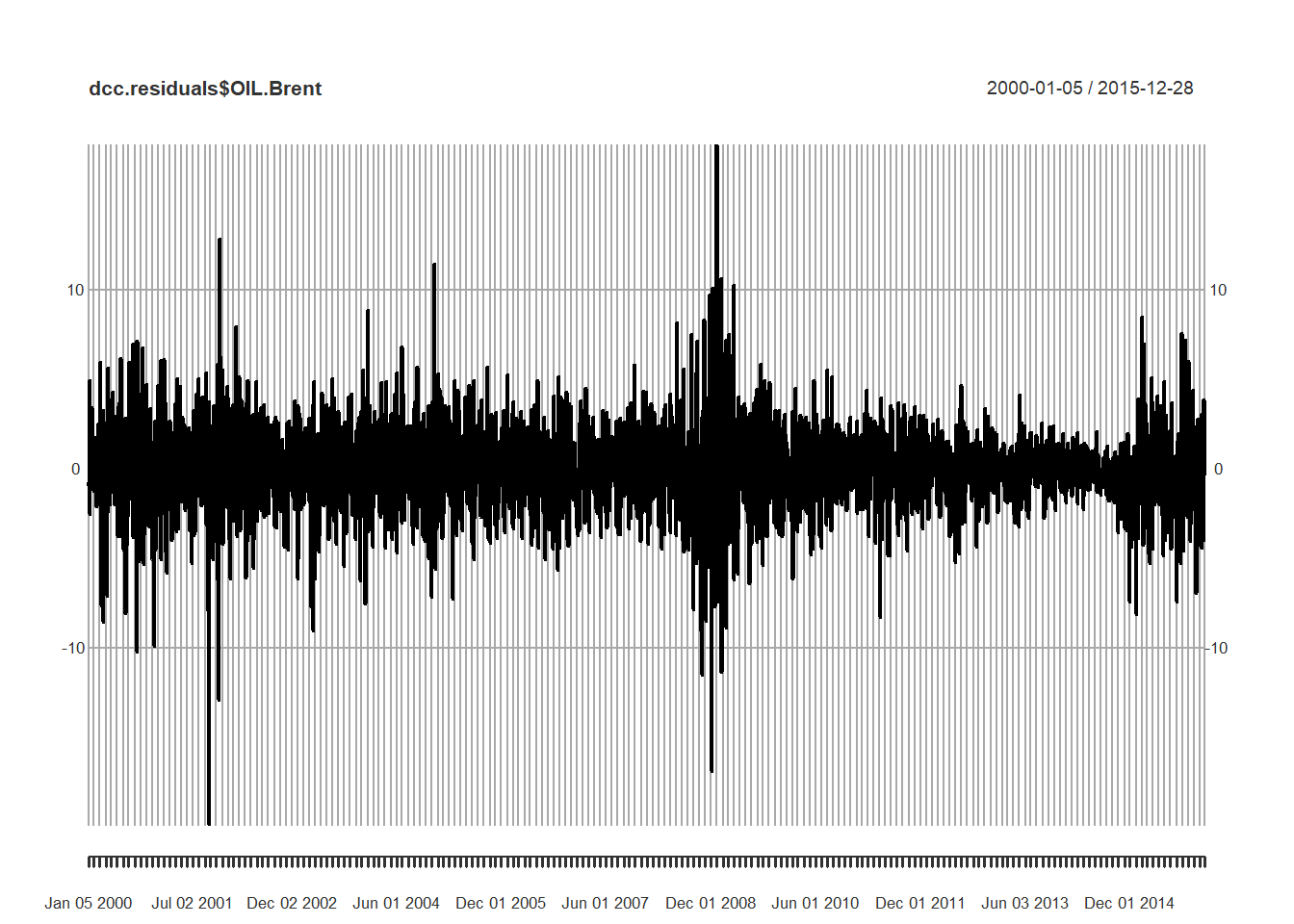

9.7 Just One More Thing

Back to Brent. Let’s refit using the new volatility models and innovation distributions to capture asymmetry and thick tails.

Brent.spec <- ugarchspec(variance.model = list(model = "gjrGARCH", 
    garchOrder = c(1, 1)), mean.model = list(armaOrder = c(1, 
    1), include.mean = TRUE), distribution.model = "nig")

Here we experiment with a new GARCH model: the gjr stands for Glosten, Jagannathan, and Runkle (1993), who proposed a volatility model that puts a knot into the works:

\[ \sigma_t^2 = \omega + \alpha \sigma_{t-1}^2 + \beta_1 \varepsilon_{t-1}^2 + \beta_2 \varepsilon_{t-1}^2 I_{t-1} \]

where \(I_{t-1} = 1\) when \(\varepsilon_{t-1} > 0\) and 0 otherwise, the “knot.”

We also experiment with a new distribution: the negative inverse gamma. Thick tails abound…

fit.Brent <- ugarchfit(spec = Brent.spec, 
    data = R$OIL.Brent, solver.control = list(trace = 0))

Another 10 seconds (or so) of our lives will fit this model.

fit.Brent

## 
## *---------------------------------*
## *          GARCH Model Fit        *
## *---------------------------------*
## 
## Conditional Variance Dynamics    
## -----------------------------------
## GARCH Model  : gjrGARCH(1,1)
## Mean Model   : ARFIMA(1,0,1)
## Distribution : nig 
## 
## Optimal Parameters
## ------------------------------------
##         Estimate  Std. Error     t value Pr(>|t|)
## mu     -0.040275    0.027883 -1.4445e+00 0.148608
## ar1     0.996072    0.001900  5.2430e+02 0.000000
## ma1    -0.989719    0.000005 -1.8786e+05 0.000000
## omega   0.006346    0.003427  1.8517e+00 0.064071
## alpha1  0.009670    0.003841  2.5178e+00 0.011808
## beta1   0.968206    0.001237  7.8286e+02 0.000000
## gamma1  0.042773    0.007183  5.9547e+00 0.000000
## skew   -0.120184    0.032059 -3.7488e+00 0.000178
## shape   2.362890    0.351494  6.7224e+00 0.000000
## 
## Robust Standard Errors:
##         Estimate  Std. Error     t value Pr(>|t|)
## mu     -0.040275    0.030871 -1.3046e+00 0.192023
## ar1     0.996072    0.002107  4.7283e+02 0.000000
## ma1    -0.989719    0.000005 -1.8363e+05 0.000000
## omega   0.006346    0.003388  1.8729e+00 0.061086
## alpha1  0.009670    0.004565  2.1184e+00 0.034143
## beta1   0.968206    0.000352  2.7485e+03 0.000000
## gamma1  0.042773    0.008503  5.0300e+00 0.000000
## skew   -0.120184    0.033155 -3.6249e+00 0.000289
## shape   2.362890    0.405910  5.8212e+00 0.000000
## 
## LogLikelihood : -8508.439 
## 
## Information Criteria
## ------------------------------------
##                    
## Akaike       4.1989
## Bayes        4.2129
## Shibata      4.1989
## Hannan-Quinn 4.2038
## 
## Weighted Ljung-Box Test on Standardized Residuals
## ------------------------------------
##                         statistic p-value
## Lag[1]                      1.856  0.1730
## Lag[2*(p+q)+(p+q)-1][5]     2.196  0.9090
## Lag[4*(p+q)+(p+q)-1][9]     2.659  0.9354
## d.o.f=2
## H0 : No serial correlation
## 
## Weighted Ljung-Box Test on Standardized Squared Residuals
## ------------------------------------
##                         statistic  p-value
## Lag[1]                     0.5109 0.474739
## Lag[2*(p+q)+(p+q)-1][5]    9.3918 0.013167
## Lag[4*(p+q)+(p+q)-1][9]   13.2753 0.009209
## d.o.f=2
## 
## Weighted ARCH LM Tests
## ------------------------------------
##             Statistic Shape Scale  P-Value
## ARCH Lag[3]     10.26 0.500 2.000 0.001360
## ARCH Lag[5]     10.41 1.440 1.667 0.005216
## ARCH Lag[7]     11.06 2.315 1.543 0.010371
## 
## Nyblom stability test
## ------------------------------------
## Joint Statistic:  2.5309
## Individual Statistics:              
## mu     0.91051
## ar1    0.07050
## ma1    0.06321
## omega  0.70755
## alpha1 0.22126
## beta1  0.28137
## gamma1 0.17746
## skew   0.25115
## shape  0.16545
## 
## Asymptotic Critical Values (10% 5% 1%)
## Joint Statistic:          2.1 2.32 2.82
## Individual Statistic:     0.35 0.47 0.75
## 
## Sign Bias Test
## ------------------------------------
##                    t-value    prob sig
## Sign Bias           1.1836 0.23663    
## Negative Sign Bias  0.7703 0.44119    
## Positive Sign Bias  1.8249 0.06809   *
## Joint Effect        9.8802 0.01961  **
## 
## 
## Adjusted Pearson Goodness-of-Fit Test:
## ------------------------------------
##   group statistic p-value(g-1)
## 1    20     27.42      0.09520
## 2    30     46.32      0.02183
## 3    40     58.50      0.02311
## 4    50     70.37      0.02431
## 
## 
## Elapsed time : 6.630391

9.7.1 Example (last one!)

Let’s run this code and recall what the evir package does for us.

require(evir)
Brent.resid <- abs(residuals(fit.Brent))
gpdfit.Brent <- gpd(Brent.resid, threshold = quantile(Brent.r, 
    0.9))
(Brent.risk <- riskmeasures(gpdfit.Brent, 
    c(0.9, 0.95, 0.975, 0.99, 0.999)))

We can interpret the results…and use the tailplot() function as well.

require(evir)
Brent.resid <- abs(residuals(fit.Brent))
gpdfit.Brent <- gpd(Brent.resid, threshold = quantile(Brent.r, 
    0.9))
(Brent.risk <- riskmeasures(gpdfit.Brent, 
    c(0.9, 0.95, 0.975, 0.99, 0.999)))

##          p  quantile     sfall
## [1,] 0.900  3.478474  5.110320
## [2,] 0.950  4.509217  6.293461
## [3,] 0.975  5.636221  7.587096
## [4,] 0.990  7.289163  9.484430
## [5,] 0.999 12.415553 15.368772

What does this mean? 1. 1 - p gives us levels of tolerance 2. quantile gives us the value at risk (VaR) 3. sfall reports the expected short fall (ES)

From the evir package here is the tail plot.

tailplot(gpdfit.Brent)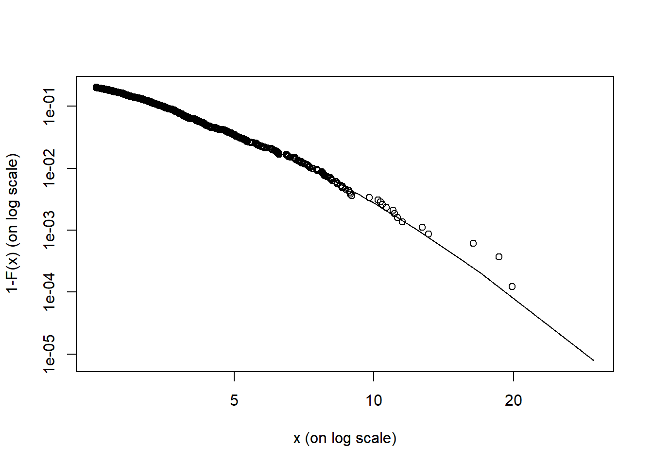

What does this mean?

• The results show much thick and volatile tail activity event with the AR-GARCH treatment.
• We could well go back to market and operational risk sections to understand mean excess value (beyond thresholds) and the confidence intervals for VaR and ES.
• For accounts receivable mitigation strategies might be to have excess risk hedges provided through reinsurance and total return swaps.
• Credit risk analysis of customers is critical: frequent updates of Brent exposed customers will help to detect early on problems that might admit of some solution.

9.8 Summary

• Lots more R practice
• Univariate GARCH
• Multivariate GARCH
• Fitting models
• Simulating volatility and correlation
• …and why it might all matter: answering a critical business question of how much volatility do we have to manage.

9.9 Further Reading

9.10 Practice Laboratory

9.10.1 Practice laboratory #1

9.10.1.1 Problem

9.10.1.2 Questions

9.10.2 Practice laboratory #2

9.10.2.1 Problem

9.10.2.2 Questions

9.11 Project

9.11.1 Background

9.11.2 Data

9.11.3 Workflow

9.11.4 Assessment

We will use the following rubric to assess our performance in producing analytic work product for the decision maker.

• The text is laid out cleanly, with clear divisions and transitions between sections and sub-sections. The writing itself is well-organized, free of grammatical and other mechanical errors, divided into complete sentences, logically grouped into paragraphs and sections, and easy to follow from the presumed level of knowledge.

• All numerical results or summaries are reported to suitable precision, and with appropriate measures of uncertainty attached when applicable.

• All figures and tables shown are relevant to the argument for ultimate conclusions. Figures and tables are easy to read, with informative captions, titles, axis labels and legends, and are placed near the relevant pieces of text.

• The code is formatted and organized so that it is easy for others to read and understand. It is indented, commented, and uses meaningful names. It only includes computations which are actually needed to answer the analytical questions, and avoids redundancy. Code borrowed from the notes, from books, or from resources found online is explicitly acknowledged and sourced in the comments. Functions or procedures not directly taken from the notes have accompanying tests which check whether the code does what it is supposed to. All code runs, and the R Markdown file knits to pdf_document output, or other output agreed with the instructor.

• Model specifications are described clearly and in appropriate detail. There are clear explanations of how estimating the model helps to answer the analytical questions, and rationales for all modeling choices. If multiple models are compared, they are all clearly described, along with the rationale for considering multiple models, and the reasons for selecting one model over another, or for using multiple models simultaneously.

• The actual estimation and simulation of model parameters or estimated functions is technically correct. All calculations based on estimates are clearly explained, and also technically correct. All estimates or derived quantities are accompanied with appropriate measures of uncertainty.

• The substantive, analytical questions are all answered as precisely as the data and the model allow. The chain of reasoning from estimation results about the model, or derived quantities, to substantive conclusions is both clear and convincing. Contingent answers (for example, “if X, then Y , but if A, then B, else C”) are likewise described as warranted by the model and data. If uncertainties in the data and model mean the answers to some questions must be imprecise, this too is reflected in the conclusions.

• All sources used, whether in conversation, print, online, or otherwise are listed and acknowledged where they used in code, words, pictures, and any other components of the analysis.

9.12 References