Chapter 7 Credit Risk

7.1 Imagine This

Our company is trying to penetrate a new market. To do so it acquires several smaller competitors for your products and services. As we acquire the companies , we also acquire their customers…and now our customers’ ability to pay us.

Not only that, but yowe have also taken your NewCo’s supply chain. Your company also has to contend with the credit worthiness of NewCo’s vendors. If they default you don’t get supplied, you can’t produce, you can’t fulfill your customers, they walk.
Your CFO has handed you the job of organizing your accounts receivable, understanding your customers’ paying patterns, and more importantly their defaulting patterns.

Some initial questions come to mind:

What are the key business questions you should ask about your customers’ paying / defaulting patterns?
What systematic approach might you use to manage customer and counterparty credit risk?

Some ideas to answer these questions can be

Key business questions might be

What customers and counterparties default more often than others?
If customer default what can we recover?
What is the total exposure that we experience at any given point in time?
How far can we go with customers that might default?

Managing credit risk

Set up a scoring system to accept new customers and track existing customers
Monitor transitions of customers from one rating notch to another
Build in early warning indicators of customer and counterparty default
Build a playbook to manage the otherwise insurgent and unanticipated credit events that can overtake your customers and counterparties

Topics we got to in the last several chapters:

Explored stylized fact of financial market data
Learned just how insidious volatility really is
Acquired new tools like acf, pacf, ccf to explore time series.

In this chapter on credit risk We Will Use actual transaction and credit migration data to examine relationships among default and explanations of credit-worthiness. We will also simulate default probababilities using markov chains. With this technology in hand we can then begin to Understand hazard rates and the probabality of transitioning from one credit state to another. Then we have a first stab a predicting default and generating loss distributions for portfolios of credit exposures, as in the the Newco example of the accounts receivable credit portfolio.

7.2 New customers!

Not so fast! Let’s load the credit profiles of our newly acquired customers. Here is what was collected these past few years:

firm.profile <- read.csv("data/creditfirmprofile.csv")
head(firm.profile)

##   id start.year default  wcTA  reTA ebitTA mktcapTL   sTA
## 1  1       2010       0 0.501 0.307  0.043    0.956 0.335
## 2  1       2011       0 0.550 0.320  0.050    1.060 0.330
## 3  1       2012       0 0.450 0.230  0.030    0.800 0.250
## 4  1       2013       0 0.310 0.190  0.030    0.390 0.250
## 5  1       2014       0 0.450 0.220  0.030    0.790 0.280
## 6  1       2015       0 0.460 0.220  0.030    1.290 0.320

Recorded for each of several years from 2006 through 2015 each firm’s (customer’s) indicator as to whether they defaulted or not (1 or 0).

summary(firm.profile)

##        id          start.year      default           wcTA        
##  Min.   :  1.0   Min.   :2006   Min.   :0.000   Min.   :-2.2400  
##  1st Qu.:192.0   1st Qu.:2009   1st Qu.:0.000   1st Qu.: 0.0300  
##  Median :358.0   Median :2011   Median :0.000   Median : 0.1200  
##  Mean   :356.3   Mean   :2011   Mean   :0.018   Mean   : 0.1426  
##  3rd Qu.:521.0   3rd Qu.:2013   3rd Qu.:0.000   3rd Qu.: 0.2400  
##  Max.   :830.0   Max.   :2015   Max.   :1.000   Max.   : 0.7700  
##       reTA             ebitTA            mktcapTL           sTA        
##  Min.   :-3.3100   Min.   :-0.59000   Min.   : 0.020   Min.   :0.0400  
##  1st Qu.: 0.0900   1st Qu.: 0.04000   1st Qu.: 0.620   1st Qu.:0.1700  
##  Median : 0.2200   Median : 0.05000   Median : 1.140   Median :0.2600  
##  Mean   : 0.2104   Mean   : 0.05181   Mean   : 1.954   Mean   :0.3036  
##  3rd Qu.: 0.3700   3rd Qu.: 0.07000   3rd Qu.: 2.240   3rd Qu.:0.3700  
##  Max.   : 1.6400   Max.   : 0.20000   Max.   :60.610   Max.   :5.0100

Several risk factors can contribute to credit risk:

Working Capital risk is measured by the Working Capital / Total Assets ratio wcTA. When this ratio is zero, current assets are matched by current liabilities. When positive (negative), current assets are greater (lesser) than current liabilities. The risk is that there are very large current assets of low quality to feed revenue cash flow. Or the risk is that there are high current liabilities balances creating a hole in the cash conversion cycle and thus a possibility of low than expected cash flow.
Internal Funding risk is measured by the Retained Earnings / Total Assets ratio reTA. Retained Earnings measures the amount of net income plowed back into the organization. High ratios signal strong capability to fund projects with internally generated cash flow. The risk is that if the organization faces extreme changes in the market place, there is not enough internally generated funding to manage the change.
Asset Profitability risk is measured by EBIT / Total Assets ratio. This is the return on assets used to value the organization. The risk is that

EBIT is too low or even negative and thus the assets are not productively reaching revenue markets or efficiently using the supply change, or both, all resulting in too low a cash flow to sustain operations and investor expectations, and
This metric falls short of investors minimum required returns, and thus investors’ expectations are dashed to the ground, they sell your stock, and with supply and demand simplicity your stock price falls, along with your equity-based compensation.

Capital Structure risk is measured by the Market Value of Equity / Total Liabilities ratio mktcapTL. If this ratio deviates from industry norms, or if too low, then shareholder claims to cash flow, and thus control of funding for responding to market changes will be impaired. The risk is similar to Internal Fund Risk but carries the additional market perception that the organization is unwilling or unable to manage change.
Asset Efficiency risk is measured by the Sales / Total Assets ratio sTA. If too low then the organization risks two things: being able to support sales with assets, and the overburden of unproductive assets unable to support new projects through additions to retained earnings or in meeting liability committments.

Let’s also load customer credit migration data. This data records the start rating, end rating and timing for each of 830 customers as their business, and the recession, affected them.

firm.migration <- read.csv("data/creditmigration.csv")
head(firm.migration)

##   id start.date start.rating end.date end.rating time start.year end.year
## 1  1      40541            6    42366          6 1825       2010     2015
## 2  2      41412            6    42366          6  954       2013     2015
## 3  3      40174            5    40479          6  305       2009     2010
## 4  3      40479            6    40905          5  426       2010     2011
## 5  3      40905            5    42366          5 1461       2011     2015
## 6  4      40905            5    41056          6  151       2011     2012

Notice that the dates are given in number of days from January 1, 1900. Ratings are numerical.

summary(firm.migration)

##        id          start.date     start.rating      end.date    
##  Min.   :  1.0   Min.   :39951   Min.   :1.000   Min.   :39960  
##  1st Qu.:230.0   1st Qu.:40418   1st Qu.:3.000   1st Qu.:41170  
##  Median :430.0   Median :40905   Median :4.000   Median :42143  
##  Mean   :421.8   Mean   :40973   Mean   :4.041   Mean   :41765  
##  3rd Qu.:631.0   3rd Qu.:41421   3rd Qu.:5.000   3rd Qu.:42366  
##  Max.   :830.0   Max.   :42366   Max.   :8.000   Max.   :42366  
##  NA's   :1709    NA's   :1709    NA's   :1709    NA's   :1709   
##    end.rating         time          start.year      end.year   
##  Min.   :1.000   Min.   :   0.0   Min.   :2009   Min.   :2009  
##  1st Qu.:3.000   1st Qu.: 344.0   1st Qu.:2010   1st Qu.:2012  
##  Median :4.000   Median : 631.0   Median :2011   Median :2015  
##  Mean   :4.121   Mean   : 791.5   Mean   :2012   Mean   :2014  
##  3rd Qu.:5.000   3rd Qu.:1157.0   3rd Qu.:2013   3rd Qu.:2015  
##  Max.   :8.000   Max.   :2415.0   Max.   :2015   Max.   :2015  
##  NA's   :1709    NA's   :1709     NA's   :1709   NA's   :1709

firm.migration <- na.omit(firm.migration)
## firm.migration$start.rating <-
## levels(firm.migration$start.rating)
## firm.migration$end.rating <-
## levels(firm.migration$end.rating)
firm.migration$time <- as.numeric(firm.migration$time)

An interesting metric is in firm.migration$time. This field has records of the difference between end.date and start.date in days between start ratings and end ratings.

hist(firm.migration$time)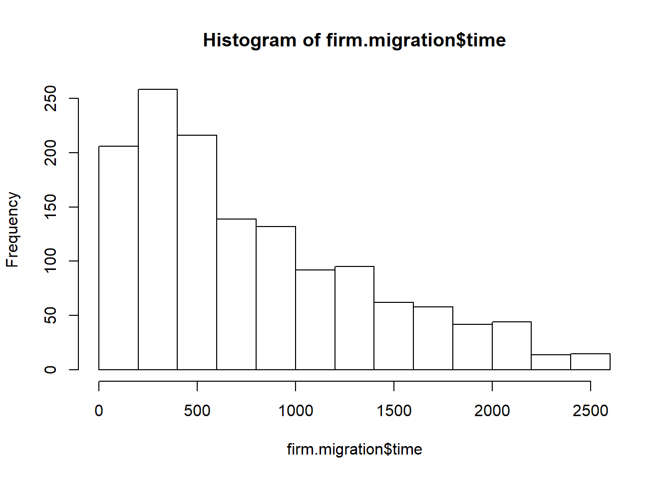

Let’s now merge the two credit files by starting year. This will (“inner”) join the data so we can see what customer conditions might be consistent with a rating change and rating dwell time. Two keys are id and start.year. The resulting data set will have records less than or equal to (if a perfect match) the maximum number of records (rows) in any input data set.

firm.credit <- merge(firm.profile, firm.migration, 
    by = c("id", "start.year"))
head(firm.credit)

##    id start.year default  wcTA  reTA ebitTA mktcapTL   sTA start.date
## 1   1       2010       0 0.501 0.307  0.043    0.956 0.335      40541
## 2  10       2014       0 0.330 0.130  0.030    0.330 0.140      42001
## 3 100       2010       0 0.170 0.240  0.080    5.590 0.270      40510
## 4 100       2013       0 0.140 0.260  0.020    2.860 0.260      41635
## 5 106       2013       0 0.040 0.140  0.060    0.410 0.320      41605
## 6 106       2013       0 0.040 0.140  0.060    0.410 0.320      41421
##   start.rating end.date end.rating time end.year
## 1            6    42366          6 1825     2015
## 2            5    42366          5  365     2015
## 3            4    41635          3 1125     2013
## 4            3    42366          3  731     2015
## 5            5    42366          5  761     2015
## 6            6    41605          5  184     2013

dim(firm.credit)

## [1] 714  14

7.2.1 Try this exercise

The shape of firm.migration$time suggests a gamma or an exponential function. But before we go off on that goose chase, let’s look at the inner-joined data to see potential differences in rating. Let’s reuse this code from previous work:

library(dplyr)

## 1: filter to keep one state. Not
## needed (yet...)
pvt.table <- firm.credit  ## filter(firm.credit, xxx %in% 'NY')

## 2: set up data frame for by-group
## processing.
pvt.table <- group_by(pvt.table, default, 
    end.rating)

## 3: calculate the three summary
## metrics
options(dplyr.width = Inf)  ## to display all columns
pvt.table <- summarise(pvt.table, time.avg = mean(time)/365, 
    ebitTA.avg = mean(ebitTA), sTA.avg = mean(sTA))

Now we display the results in a nice table

knitr::kable(pvt.table)

default	end.rating	time.avg	ebitTA.avg	sTA.avg
0	1	3.021005	0.0491667	0.2633333
0	2	2.583007	0.0529762	0.3250000
0	3	2.468776	0.0520103	0.2904124
0	4	2.106548	0.0455495	0.2655495
0	5	1.912186	0.0501042	0.2883333
0	6	1.697821	0.0504886	0.3041477
0	7	1.672251	0.0494286	0.3308571
0	8	2.467123	0.0591667	0.3208333
1	1	2.413699	-0.0100000	0.4100000
1	2	2.497717	0.0216667	0.2683333
1	3	2.613699	0.0200000	0.2400000
1	6	2.242466	0.0350000	0.1150000
1	7	3.002740	0.0500000	0.3000000

Defaulting (default = 1)firms have very low EBIT returns on Total Assets as well as low Sales to Total Assets… as expected. They also spent a lot of time (in 365 day years) in rating 7 – equivalent to a “C” rating at S&P.

Now let’s use the credit migration data to understand the probability of default as well as the probabilities of being in other ratings or migrating from one rating to another.

7.3 It Depends

Most interesting examples in probability have a little dependence added in: “If it rained yesterday, what is the probability it rains today?” We can use this idea to generate weather patterns and probabilities for some time in the future.

In market risk, we can use this idea to generate the persistence of consumption spending, inflation, and the impact on zero coupon bond yields.
In credit, dependence can be seen in credit migration: if an account receivable was A rated this year, what are the odds this receivable be A rated next year?

We will use a mathematical representation of these language statements to help us understand the dynamics of probabalistic change we so often observe in financial variables such as credit default.

7.3.1 Enter A.A Markov

Suppose we have a sequence of $T$ observations, $\{X_t\}_{1}^{T}$, that are dependent. In a time series, what happens next can depend on what happened before:

\[ p(X_1, X_2, ..., X_T) = p(X_1)p(X_2|X_1)...p(X_t|X_{t-1},...,X_1) \]

Here $p(x|y)$ is probability that an event $x$ (e.g., default) occurs whenever (the vertical bar |) event $y$ occurs. This is the statement of conditional probability. Event $x$ depends in some way on the occurrence of $y$.

With markov dependence each outcome only depends on the one that came before.

\[ p(X_1, X_2, ..., X_T) = p(X_1)\prod_{s=2}^T p(X_s|X_{s-1}) \]

We have already encountered this when we used the functions acf and ccf to explore very similar dependencies in macro-financial time series data. In those cases we explored the dependency of today’s returns on yesterday’s returns. Markov dependence is equivalent to an AR(1) process (today = some part of yesterday plus some noise).

To generate a markov chain, we need to do three things:

Set up the conditional distribution.
Draw the initial state of the chain.
For every additional draw, use the previous draw to inform the new one.

Now we are a position to develop a very simple (but oftentimes useful) credit model:

If a receivable’s issuer (a customer) last month was investment grade, this month’s chance of also being investment grade is 80%.
If a receivable’s issuer last month was not investment grade, this month’s chance of being investment grade is 20%.

7.3.2 Try this exercise

We will simulate monthly for 5 years. Here we parameterize even the years and calculate the number of months in the simulation. We set up a dummy investment.grade variable with NA entries into which we deposit 60 dependent coin tosses using the binomial distribution. The probability of success (state = “Investment Grade”) is overall 80% and is composed of a long run 20% (across the 60 months) plus a short run 60% (of the previous month). Again the similarity to an autoregressive process here with lags at 1 month and 60 months.

Then,

We will run the following code.
We should look up rbinom(n, size, prob) (coin toss random draws) to see the syntax.
We will interpret what happens when we set the long.run rate to 0% and the short.run rate to 80%.

N.years <- 5
N.months <- N.years * 12
investment.grade <- rep(NA, N.months)
investment.grade[1] <- 1
long.run <- 0.5
short.run <- 0
for (month in 2:N.months) {
    investment.grade[month] <- rbinom(1, 
        1, long.run + short.run * investment.grade[month - 
            1])
}
hist(investment.grade)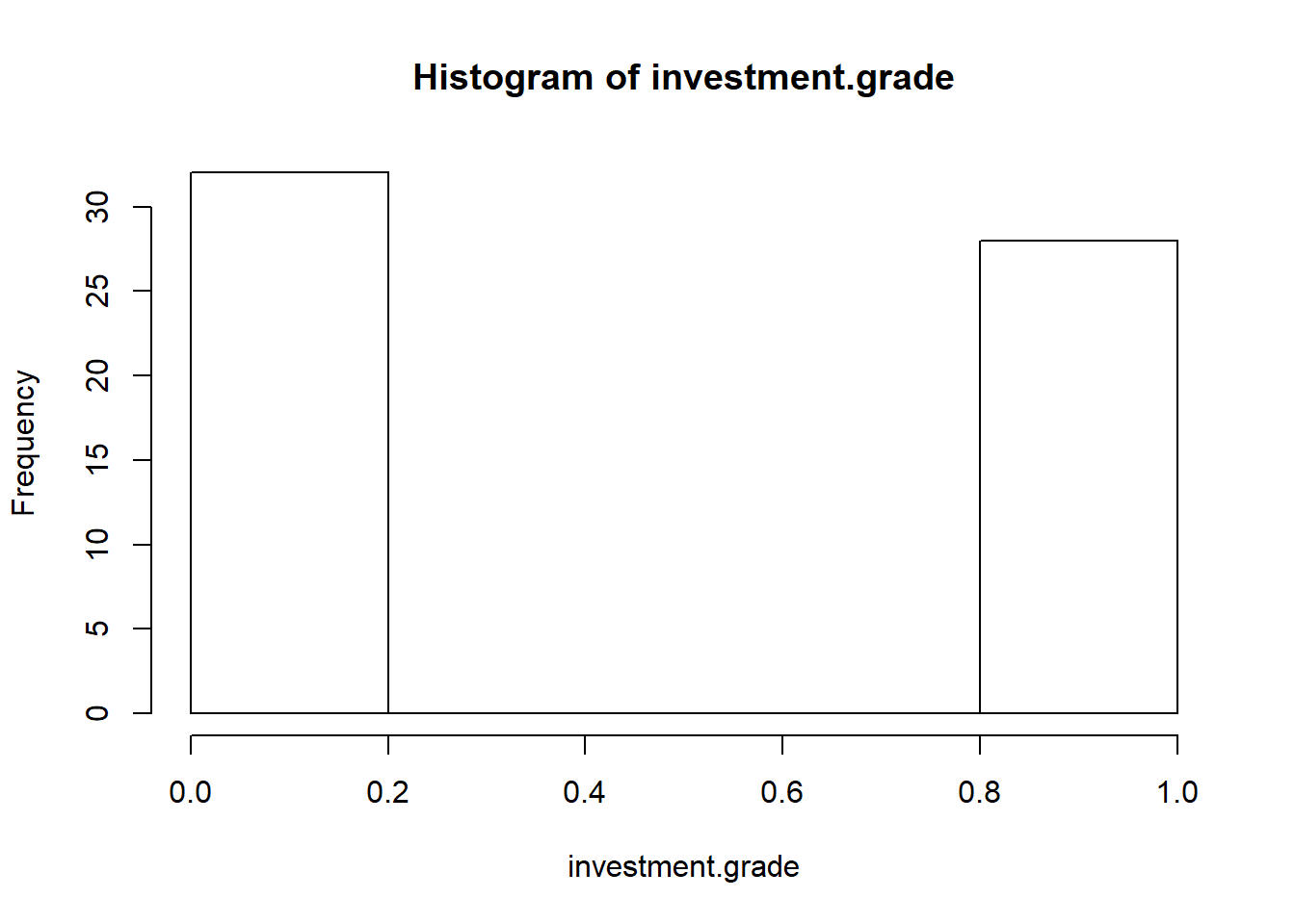

The for (month in 2:N.months) loop says “For each month starting at month 2, perform the tasks in the curly brackets ({}) until, and including, N.months”

Almost evenly ditributed probabilities occur. We plot the results.

plot(investment.grade, main = "Investment Grade", 
    xlab = "Month", ylab = "IG?", ty = "s")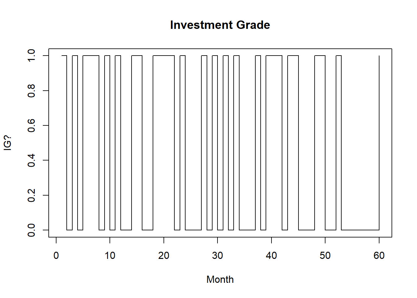

Now to look at a scenario with long-run = 0.0, and short-run = 0.80

N.years <- 5
N.months <- N.years * 12
investment.grade <- rep(NA, N.months)
investment.grade[1] <- 1
long.run <- 0  ## changed from base scenario 0.5
short.run <- 0.8  ## changed from base scenario 0.0
for (month in 2:N.months) {
    investment.grade[month] <- rbinom(1, 
        1, long.run + short.run * investment.grade[month - 
            1])
}
hist(investment.grade)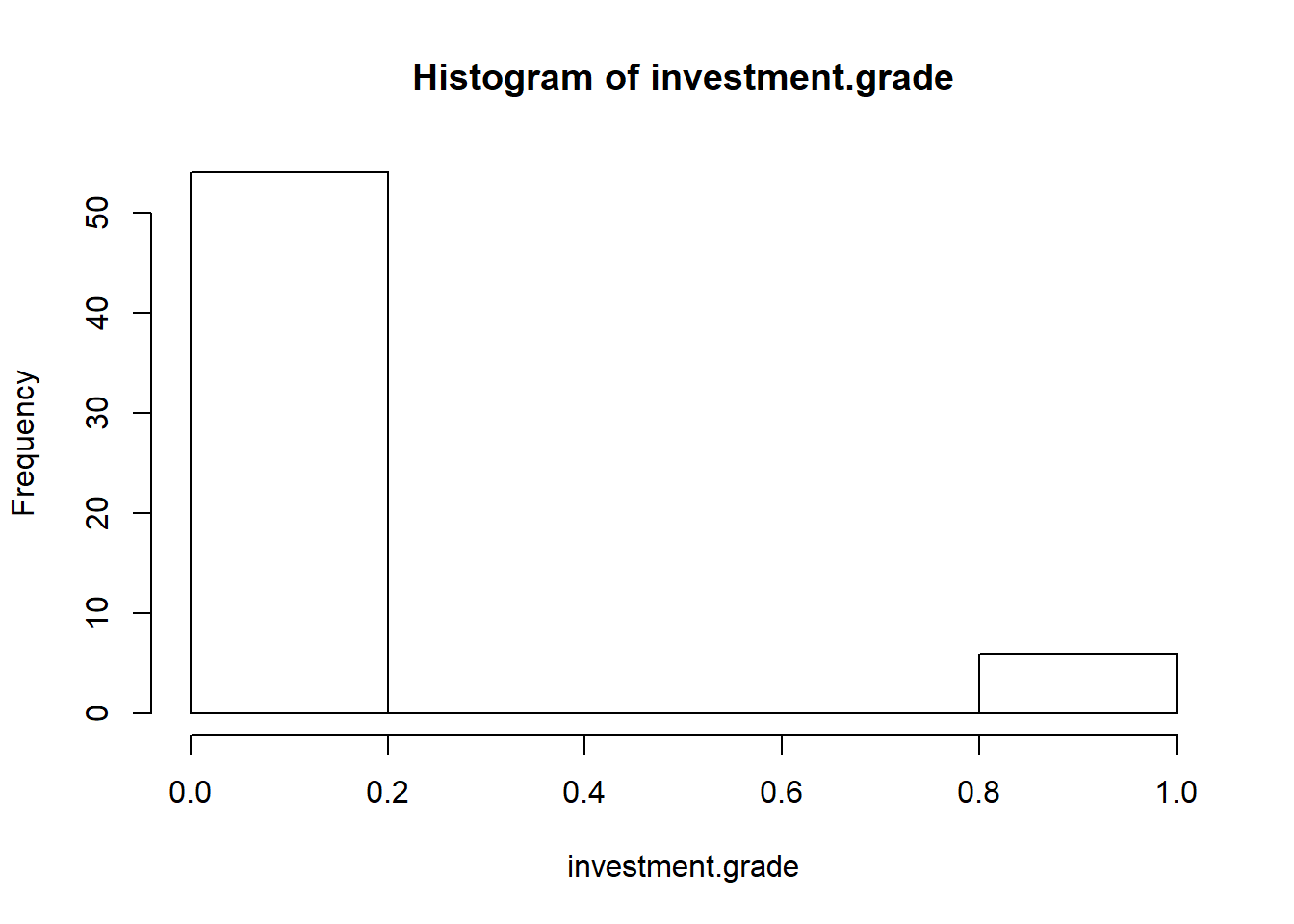

The result is much different now with more probability concentrated in lower end of investment grade scale. The next plot the up and down transitions between investment grade and not-investment grade using lines to connect up to down transitions. Now this looks more like a bull and bear graph.

plot(investment.grade, main = "Investment Grade", 
    xlab = "Month", ylab = "IG?", ty = "l")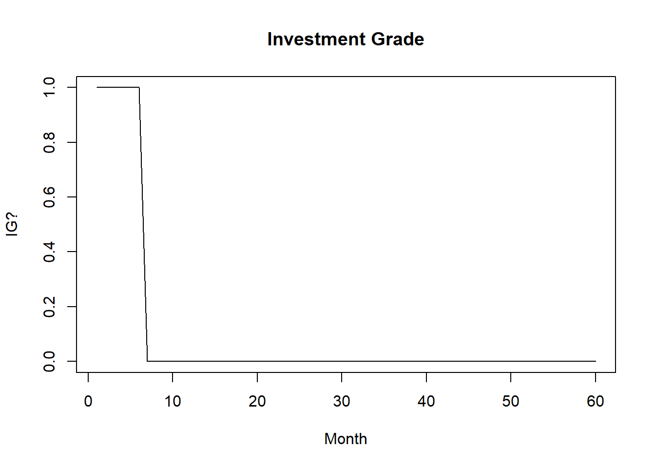

And we see how different these transitions are from a simple coin toss credit model (independence, not dependence). We could just set the long.run rate to 50% (a truly unbiased coin) and rerun, or simply run the following.

toss.grade <- rbinom(N.months, 1, 0.5)
plot(toss.grade, main = "Investment Grades (yawn!)", 
    xlab = "Month", ylab = "IG?", ty = "l")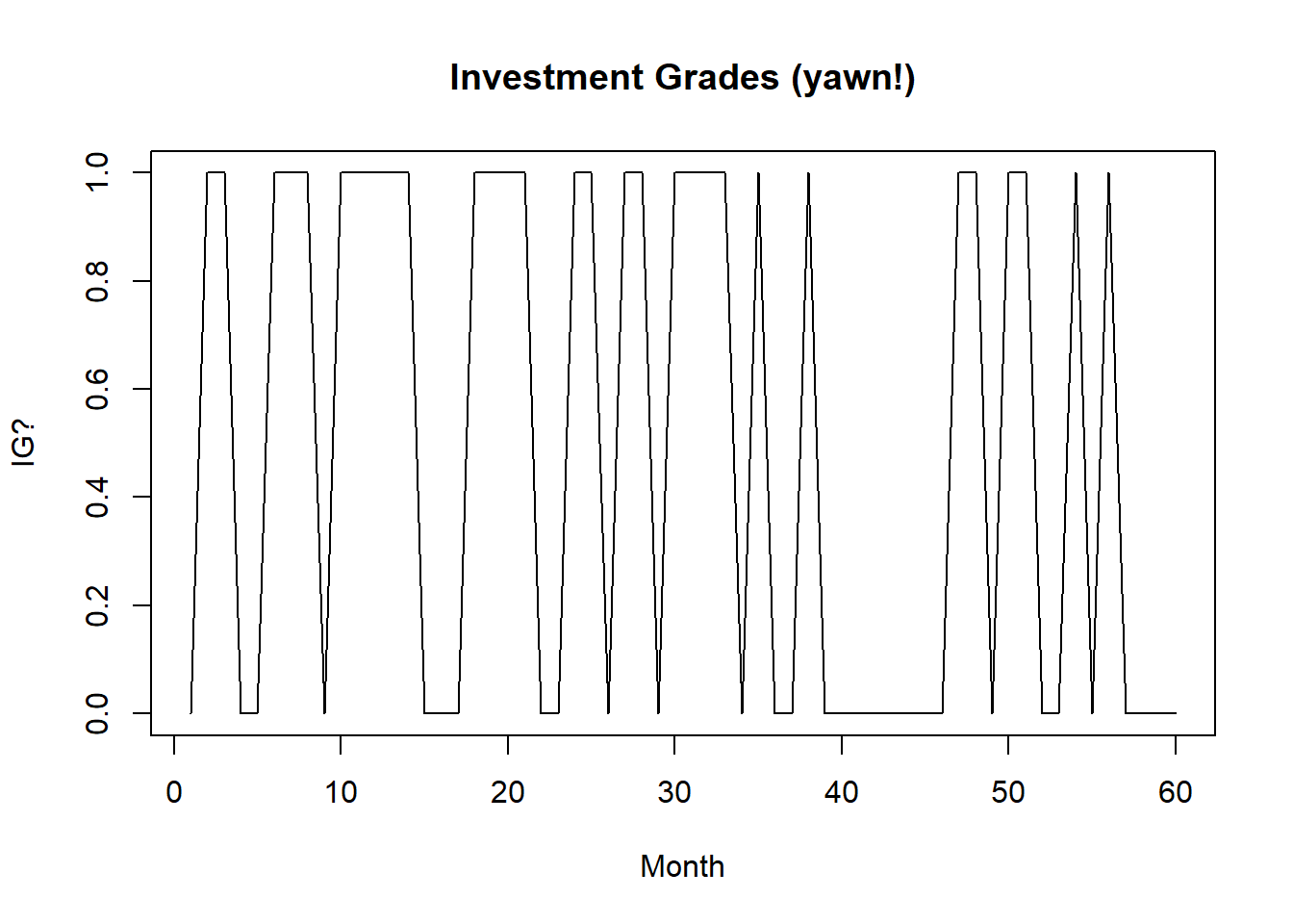

In our crude credit model transitions are represented as a matrix: $Q_{ij}$ is $P(X_t = j|X_{t-1} = i)$ where, $i$ is the start state (“Investment Grade”), and $j$ is the end state (“not-Investment Grade”). Here is a transition matrix to encapsulate this data.

(transition.matrix <- matrix(c(0.8, 0.2, 
    0.2, 0.8), nrow = 2))

##      [,1] [,2]
## [1,]  0.8  0.2
## [2,]  0.2  0.8

This function will nicely simulate this and more general random Markov chains.

rmarkovchain <- function(n.sim, transition.matrix, 
    start = sample(1:nrow(transition.matrix), 
        1)) {
    result <- rep(NA, n.sim)
    result[1] <- start
    for (t in 2:n.sim) result[t] <- sample(ncol(transition.matrix), 
        1, prob = transition.matrix[result[t - 
            1], ])
    return(result)
}

7.3.3 Try this next exercise

Let’s run a 1000 trial markov chain with the 2-state transition.matrix and save to a variable called ‘markov.sim’. Then we will use the table function to calculate how many 1’s and 2’ are simulated.

Many trials (and tribulations…) follow from this code.

markov.sim <- rmarkovchain(1000, transition.matrix)
head(markov.sim)

## [1] 2 1 1 1 1 2

Then we tabulate the contingency table.

ones <- which(markov.sim[-1000] == 1)
twos <- which(markov.sim[-1000] == 2)
state.one <- signif(table(markov.sim[ones + 
    1])/length(ones), 3)
state.two <- signif(table(markov.sim[twos + 
    1])/length(twos), 3)
(transition.matrix.sim <- rbind(state.one, 
    state.two))

##               1     2
## state.one 0.817 0.183
## state.two 0.220 0.780

The result is pretty close to transition.matrix. The Law of large numbers would say we converge to these values. The function which() sets up two indexes to find where the 1’s and 2’s are in markov.sim. The function signif() with 3 means use 3 significant digits. The the function table() tabulates the number of one states and two states simulated.

Next let’s develop an approach to estimating transition probabilities using observed (or these could be simulated… if we are not very sure of future trends) rates of credit migration from one rating to another.

7.4 Generating Some Hazards

Let’s set up a more realistic situation. Suppose we have annual hazard rates $\lambda$ for each of 4 in-house credit ratings for a portfolio of accounts receivable. We can use a pivot table to get these rates. Suppose that we know the number of accounts that transition from one rating (start state) to another rating (end state) in a unit of time (here a year). We define the hazard rate $\lambda$ as the number of accounts that migrate from one rating to another rating (per year) divided by the number of all the accounts that year at that starting rating.

Next we suppose we have $N$ ratings which in Markov-speak are states of being in a credit rating. Transition probabilities are summarized by a $N$ row $\times$ $N$ column “generator” matrix $\Lambda = [\lambda_{ij}]$. Here the row index is $i = 1...N$ starting credit rating states and the column index is $j = 1...N$ ending credit rating states for a customer.

Over any small (and getting ever smaller…) time step of duration $dt$ the probability of a transition from rating i to j is given approximately by $\lambda_{ij} dt$. The probability of moving to any other rating from the starting rating is $\Sigma_{i \neq j} \lambda_{ij}$ so that staying at rating i is given by $1 - \Sigma_{i \neq j} \lambda_{ij}$ all along the diagonal of the matrix.

A little more formally, and usefully, we can define for transitions from a starting state rating $i$ to an ending state rating $j$ over an interval of time $s = [0,t]$, the hazard rate for $i \neq j$,

\[ \lambda_{ij} = \frac{N_{ij}}{\int_{0}^{t} Y_{i}(s) ds} \]

where $N_{ij}$ is the number of accounts that made the transition from one rating $i$ to another, different rating $j$, and $Y_i$ is the number of accounts rated in the starting state rating $i$ at the beginning of the time interval $(t, t + dt)$.

The int sign is again (remember the term structure of interest rates) the cumulative sum of the product of the number of accounts times the time an account is in a transition from one credit rating state to another. Using this formula, the math to generate ratings migration probabilities is fairly straightforward with a couple of kinks.

The probability of transitions is $P = exp( \Lambda)$. We can think of probabilities as discounts. They range from 0 to 1 like the present value of $1. $\lambda_{ij} dt$ is just like a forward interest rate in form as it is the change in probability (present value) from one date to another $dt$. We will use the expm package to calculate the matrix exponent.

First suppose we already know the hazard rates for each starting state rating. We will assign the D.rating hazard rate as a 0 throughout as this is the last state, that is, there is no transition from this rating to another rating. Then create a $\lambda$ matrix by concatenating the rows of hazard rates, and see that the diagonals are zero.

By definition, if an account stays in a rating, the diagonal must be the negative of the row sum of this matrix, where we use the apply function on the first, the row, dimension of the matrix. We put the negative row sum into the diagonal and now we have a proper hazard, or also called generator, matrix.

Now, for the last step here, we raise the hazard matrix to the exponent power. The result is the probability transition matrix.

require(Matrix)
rating.names <- c("A1", "A2", "A3", "B1", 
    "B2", "B3", "C", "D")
lambda <- structure(c(-0.08179, 0.00663, 
    6e-04, 0.00035, 0.00029, 0, 0.000815871122518043, 
    0, 0.07493, -0.093, 0.02029, 0.002, 
    0.00088, 0.00076, 0, 0, 0.00515, 
    0.08159, -0.08697, 0.04178, 0.00441, 
    0.00229, 0.00408, 0, 0.00114404022385915, 
    0.00361106546371299, 0.0615488360753306, 
    -0.110345216529572, 0.0534942615312562, 
    0.00343192628444715, 0.0057110978576263, 
    0, 0.000572020111929575, 0.000585578183304809, 
    0.00321930968833733, 0.0588046608464803, 
    -0.176844582534647, 0.0531948574089309, 
    0.0138698090828067, 0, 0, 0.000487981819420674, 
    0.0012004205617529, 0.00615719390039617, 
    0.108360170794083, -0.190567240072496, 
    0.134618735215477, 0, 0, 9.75963638841349e-05, 
    0.000109129141977537, 0.000622637585433321, 
    0.00666228898191469, 0.102671794676377, 
    -0.828109189355814, 0, 0, 0, 0, 0.000622637585433321, 
    0.00274329546314134, 0.0282180605610099, 
    0.669014320464795, 0), dim = c(8, 
    8), dimnames = list(rating.names, 
    rating.names))
# write.csv(lambda,'data/lambdahat.csv')
# # To save this work lambda <-
# read.csv('data/lambdahat.csv')
rownames(lambda) <- c("A1", "A2", "A3", 
    "B1", "B2", "B3", "C", "D")
colnames(lambda) <- c("A1", "A2", "A3", 
    "B1", "B2", "B3", "C", "D")
apply(lambda, 1, sum)

##            A1            A2            A3            B1            B2 
##  6.060336e-06  2.221830e-06 -2.304533e-06 -8.086612e-06 -4.565764e-06 
##            B3             C             D 
## -6.011417e-07  6.443874e-07  0.000000e+00

dimnames(lambda) <- list(rating.names, 
    rating.names)
lambda.diag <- -apply(lambda, 1, sum)  ## this the is rate of staying in a state
diag(lambda) <- lambda.diag  ## this pops lambda.diag into the diagonal of lambda
apply(lambda, 1, sum)  ## should add up to zero

##        A1        A2        A3        B1        B2        B3         C 
## 0.0817900 0.0930000 0.0869700 0.1103452 0.1768446 0.1905672 0.8281092 
##         D 
## 0.0000000

P <- expm(lambda)
apply(P, 1, sum)  ## Should be ones

##       A1       A2       A3       B1       B2       B3        C        D 
## 1.085734 1.097323 1.092018 1.118836 1.195059 1.238993 1.844956 1.000000

We behold the generator matrix and its associated transition probabilities:

signif(lambda, 6)

##              A1           A2          A3          B1          B2
## A1 -6.06034e-06  7.49300e-02 5.15000e-03 1.14404e-03 5.72020e-04
## A2  6.63000e-03 -2.22183e-06 8.15900e-02 3.61107e-03 5.85578e-04
## A3  6.00000e-04  2.02900e-02 2.30453e-06 6.15488e-02 3.21931e-03
## B1  3.50000e-04  2.00000e-03 4.17800e-02 8.08661e-06 5.88047e-02
## B2  2.90000e-04  8.80000e-04 4.41000e-03 5.34943e-02 4.56576e-06
## B3  0.00000e+00  7.60000e-04 2.29000e-03 3.43193e-03 5.31949e-02
## C   8.15871e-04  0.00000e+00 4.08000e-03 5.71110e-03 1.38698e-02
## D   0.00000e+00  0.00000e+00 0.00000e+00 0.00000e+00 0.00000e+00
##             B3            C           D
## A1 0.00000e+00  0.00000e+00 0.000000000
## A2 4.87982e-04  9.75964e-05 0.000000000
## A3 1.20042e-03  1.09129e-04 0.000000000
## B1 6.15719e-03  6.22638e-04 0.000622638
## B2 1.08360e-01  6.66229e-03 0.002743300
## B3 6.01142e-07  1.02672e-01 0.028218100
## C  1.34619e-01 -6.44387e-07 0.669014000
## D  0.00000e+00  0.00000e+00 0.000000000

signif(P, 4)

## 8 x 8 Matrix of class "dgeMatrix"
##           A1        A2       A3       B1        B2        B3         C
## A1 1.000e+00 0.0750100 0.008240 0.001518 0.0006474 6.084e-05 8.586e-06
## A2 6.658e-03 1.0010000 0.081750 0.006152 0.0008909 6.040e-04 1.352e-04
## A3 6.794e-04 0.0203900 1.002000 0.061750 0.0050820 1.650e-03 2.206e-04
## B1 3.796e-04 0.0024710 0.042060 1.003000 0.0591600 9.455e-03 1.251e-03
## B2 3.089e-04 0.0010410 0.005727 0.053960 1.0050000 1.094e-01 1.228e-02
## B3 5.404e-05 0.0008185 0.002756 0.005259 0.0542200 1.010e+00 1.032e-01
## C  8.228e-04 0.0001392 0.004417 0.006528 0.0176900 1.358e-01 1.007e+00
## D  0.000e+00 0.0000000 0.000000 0.000000 0.0000000 0.000e+00 0.000e+00
##            D
## A1 3.617e-06
## A2 5.139e-05
## A3 1.065e-04
## B1 1.164e-03
## B2 7.781e-03
## B3 6.283e-02
## C  6.725e-01
## D  1.000e+00

The last row of P are all zeros until the last entry, the diagonal entry. It means if you are in “D” it is certain you stay in “D”.

Digging in we look at the non-defaulting rating distributions with thresholds for the “C” rating.

First, we order the transition probabilities from worst (D) to best (A). Then take out the worst (D).

(P.reverse <- P[4:1, 4:1])  ## Reorder from worst to best

## 4 x 4 Matrix of class "dgeMatrix"
##             B1          A3          A2           A1
## B1 1.002899527 0.042057508 0.002470551 0.0003795657
## A3 0.061752300 1.002134622 0.020393062 0.0006794168
## A2 0.006152205 0.081749969 1.001081413 0.0066579619
## A1 0.001518019 0.008239507 0.075010753 1.0002449919

(P.reverse <- P.reverse[-1, ])  ## Eliminate the D state transitions

## 3 x 4 Matrix of class "dgeMatrix"
##             B1          A3         A2           A1
## A3 0.061752300 1.002134622 0.02039306 0.0006794168
## A2 0.006152205 0.081749969 1.00108141 0.0066579619
## A1 0.001518019 0.008239507 0.07501075 1.0002449919

h Second, we compute cumulative probabilities for the C rating in the first row now. Then compute cumulative probabilities.

(C.probs <- P.reverse[1, ])

##           B1           A3           A2           A1 
## 0.0617523000 1.0021346225 0.0203930620 0.0006794168

(C.cumprobs <- pmin(0.999, pmax(0.001, 
    cumsum(C.probs))))

## [1] 0.0617523 0.9990000 0.9990000 0.9990000

Third, let’s interpret our results through an exercise.

7.4.1 Try this exercise

Now that we have gone this far let’s run the following and answer some questions about what we did.

rating.df <- 16  ## Thinking that there are 3 non-defaulting ratings being spliced together using cumulative sums to estimate hazards
(thresholds <- qt(C.cumprobs, rating.df))
threshold.plot <- data.frame(Deviation = seq(from = -5, 
    to = 15, length = 100), Density = dt(seq(from = -5, 
    to = 5, length = 100), df = rating.df))
require(ggplot2)
ggplot(threshold.plot, aes(x = Deviation, 
    y = Density)) + geom_line(colour = "blue", 
    size = 1.5) + geom_vline(xintercept = thresholds, 
    colour = "red", size = 0.75) + geom_hline(yintercept = 0)

Here are the standard deviations for each transition from C to B to A:

rating.df <- 16  ## Thinking that there are 3 non-defaulting ratings being spliced together
(thresholds <- qt(C.cumprobs, rating.df))

## [1] -1.625890  3.686155  3.686155  3.686155

We compute thresholds using a fairly thick-tailed quantiles of Gossett’ Student’s t-distribution (only 2 degrees of freedom). These thresholds are what we have been seeking: they tell us when a customer’s credit is suspect, needs to be further examined, or mitigated.

Here is the plot, where we first define a data frame suited to the task.

threshold.plot <- data.frame(Deviation = seq(from = -5, 
    to = 15, length = 100), Density = dt(seq(from = -5, 
    to = 5, length = 100), df = rating.df))
require(ggplot2)
ggplot(threshold.plot, aes(x = Deviation, 
    y = Density)) + geom_line(colour = "blue", 
    size = 1.5) + geom_vline(xintercept = thresholds, 
    colour = "red", size = 0.75) + geom_hline(yintercept = 0)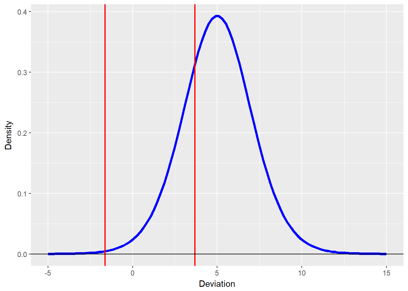

rating.df <- 16  ## Thinking that there are 3 non-defaulting ratings being spliced together
(thresholds <- qt(C.cumprobs, rating.df))
threshold.plot <- data.frame(Deviation = seq(from = -5, 
    to = 5, length = 100), Density = dt(seq(from = -5, 
    to = 5, length = 100), df = rating.df))
require(ggplot2)
ggplot(threshold.plot, aes(x = Deviation, 
    y = Density)) + geom_line(colour = "blue", 
    size = 1.5) + geom_vline(xintercept = thresholds, 
    colour = "red", size = 1.5) + geom_hline(yintercept = 0)

Again the t-distribution standard deviation thresholds:

## [1] -1.625890  3.686155  3.686155  3.686155

## [1] -1.625890  3.686155  3.686155  3.686155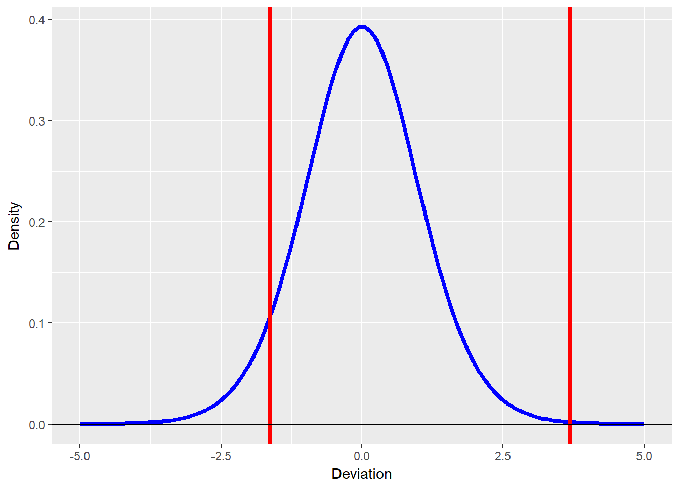

The dt in the plot is the Student’s t density function from -5 to +5 for 100 ticks.

Now that this works for one rating let’s plot all of the ratings row by row using apply with the cusum function (on the first dimension). We will use the Student’s t distribution to generate thresholds.

## Being sure we transpose this next
## result
cumprobs <- t(apply(P.reverse, 1, function(v) {
    pmin(0.999, pmax(0.001, cumsum(v)))
}))
## v holds the values of of the
## elements of each row (remember this
## is 'row-wise') we are accumulating
## a sum
rating.df <- 16
thresholds <- qt(cumprobs, rating.df)  ##Use Student's t
plot.parm <- par(mfrow = c(1, 3))  ## Building a 1 row, 3 column panel
for (j in 1:nrow(thresholds)) {
    plot(seq(from = -5, to = 5, length = 100), 
        dnorm(seq(from = -5, to = 5, 
            length = 100)), type = "l", 
        xlab = "Deviation", ylab = "Density", 
        main = paste(rownames(thresholds)[j], 
            "Rating"))
    abline(v = thresholds[j, ], col = 1:length(thresholds[j, 
        ]))
}

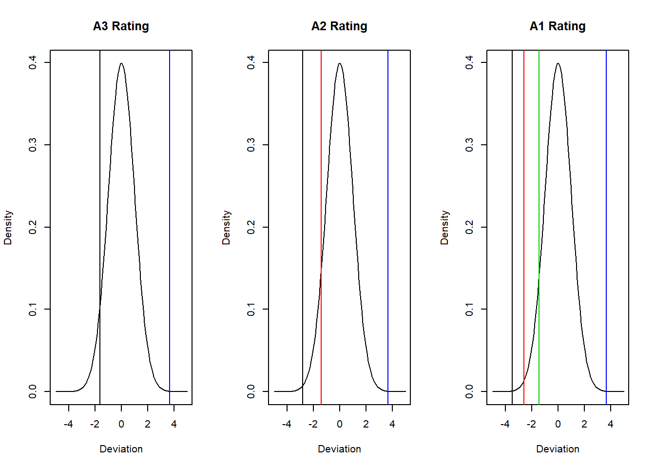
par(plot.parm)

The A ratings have a much lower loss threshold as we would expect than C or B.

7.5 Now for the Future

Decision makers now want to use this model to look into the future. Using the hazard rates to develop policies for our accounts receivable, and ultimately customer and counterparty (e.g., vendors) relationships. Let’s build a rating event simulation to dig into how these rates might occur in the wild future.

Let’s use transaction data to estimate an eight rating hazard rate to simulate the data we might have seen in the first place.

## Number of rating categories
n.cat <- dim(lambda)[1]
## Sum of migration rates from each
## non-default rating
(rates.sum <- -diag(lambda)[-n.cat])

##            A1            A2            A3            B1            B2 
##  6.060336e-06  2.221830e-06 -2.304533e-06 -8.086612e-06 -4.565764e-06 
##            B3             C 
## -6.011417e-07  6.443874e-07

## Names of non-default ratings
names.nondf <- names(rates.sum)
## probabilities of transition (off
## diagonal)
(transition.probs <- lambda[-n.cat, ]/rates.sum)

##            A1         A2         A3          B1           B2          B3
## A1   -1.00000 12364.0014   849.7879    188.7751     94.38753      0.0000
## A2 2984.02625    -1.0000 36721.9761   1625.2661    263.55666    219.6306
## A3 -260.35648 -8804.3884    -1.0000 -26707.7307  -1396.94691   -520.8955
## B1  -43.28141  -247.3224 -5166.5643     -1.0000  -7271.85403   -761.4059
## B2  -63.51620  -192.7388  -965.8843 -11716.3871     -1.00000 -23733.1944
## B3    0.00000 -1264.2609 -3809.4178  -5709.0135 -88489.70993     -1.0000
## C  1266.11897     0.0000  6331.5948   8862.8328  21524.02249 208909.6300
##                C            D
## A1       0.00000       0.0000
## A2      43.92611       0.0000
## A3     -47.35413       0.0000
## B1     -76.99610     -76.9961
## B2   -1459.18375    -600.8404
## B3 -170794.65519  -46940.7780
## C       -1.00000 1038217.5553

## matrix rows sum to zero
apply(transition.probs, 1, sum)

##         A1         A2         A3         B1         B2         B3 
##   13495.95   41857.38  -37738.67  -13645.42  -38732.75 -317008.84 
##          C 
## 1285110.75

A last row would have been the D rating absorbing row of 3 zeros and a 1.

Let’s create a miniverse of 20 years of rating migration data. This will help us understand the many possibilities for accounts receivable transitions, even through we do not have the direct data to do so. Within the 20 years we allow for up to 5 transitions per account. All of this is deposited into a data frame that will have as columns (fields in a database) an ID, a start time for the transition state, and end time for the state, followed by the starting transition and the ending transition. These fields will allow us to compute how long an account dwells in a transition state (that is, a rating).

We generate a random portfolio of 100 accounts and calculate how long it takes for them to transition from one credit rating (transition start state) to another (transition end state). We also build into the simulation fractions of accounts in each of the non-defaulting notches. These fractions serve as the first step in estimating the probability of being in a rating notch.

set.seed(1016)
n.firms <- 100
fractions <- c(0.1, 0.1, 0.1, 0.1, 0.1, 
    0.1, 0.1)  ## equal number of transitions of each rating 
initial.ratings <- sample(names.nondf, 
    size = n.firms, replace = TRUE, prob = fractions)
table(initial.ratings)

## initial.ratings
## A1 A2 A3 B1 B2 B3  C 
## 14 18 11 10 21 13 13

The table function tells us how many firms out of a 100 are in each non-default rating on average over the simulation.

Now we set up parameters for 20 years of data across the 100 firms. This will help us understand the many possibilities for accounts receivable transitions, even through we might not have enough direct data to do so. Within the 20 years we allow for up to 5 transitions per account. All of this is deposited into a data frame that will have as columns (fields in a database) an ID, a start time for the transition state, and end time for the state, followed by the starting transition and the ending transition. These fields will allow us to compute how long an account dwells in a transition state (that is, a rating).

We begin the simulation of events by creating an outer loop of firms, 100 in all in our simulated accounts receivable portfolio. We are allowing no more than 5 credit rating transitions as well.

n.years <- 10
max.row <- n.firms * 5
output.Transitions <- data.frame(id = numeric(max.row), 
    start.time = numeric(max.row), end.time = numeric(max.row), 
    start.rating = rep("", max.row), 
    end.rating = rep("", max.row), stringsAsFactors = FALSE)

The for loop simulates start and end times for each rating for each firm (up to so many transitions across so many years). Within the loop we calculate how long the firm is in each rating, until it isn’t. It is this time in transition (the “spell” or “dwell time”) that is really the core of the simulation and our understanding of hazard rate methodology. We will model this dwell time as an exponential function using rexp() to sample a time increment. Other functions we could use might be the Weibull or double-exponential for this purpose. At the end of this routine we write the results to file.

count <- 0
for (i in 1:n.firms) {
    end.time <- 0
    end.rating <- initial.ratings[i]
    while ((end.time < n.years) & (end.rating != 
        "D") & !is.na(end.time)) {
        count <- count + 1
        start.time <- end.time
        start.rating <- end.rating
        end.time <- start.time + rexp(n = 1, 
            rate = rates.sum[start.rating])
        if ((end.time <= n.years) & !is.na(end.time)) {
            pvals <- transition.probs[start.rating, 
                names.nondf != start.rating]
            end.rating <- sample(names(pvals), 
                size = 1, prob = pvals)
        }
        if ((end.time > n.years) & !is.na(end.time)) {
            end.time <- n.years
        }
        output.Transitions[count, ] <- list(i, 
            start.time, end.time, start.rating, 
            end.rating)
    }
}
write.csv(output.Transitions, "data/creditmigration.csv")

We configure all of the columns of our output data framw. We also compute the time in a rating state and add to the original output.Transitions data frame.

## output.Transitions <-
## output.Transitions[1:count,]
output.Transitions <- read.csv("data/creditmigration.csv")
output.Transitions$start.rating <- as.factor(output.Transitions$start.rating)
output.Transitions$end.rating <- as.factor(output.Transitions$end.rating)
## output.Transitions$time <-
## output.Transitions$end.time-output.Transitions$start.time
transition.Events <- output.Transitions

And then we look at the output.

head(output.Transitions)

##   id start.date start.rating end.date end.rating time start.year end.year
## 1  1      40541            6    42366          6 1825       2010     2015
## 2  2      41412            6    42366          6  954       2013     2015
## 3  3      40174            5    40479          6  305       2009     2010
## 4  3      40479            6    40905          5  426       2010     2011
## 5  3      40905            5    42366          5 1461       2011     2015
## 6  4      40905            5    41056          6  151       2011     2012

Let’s inspect our handiwork further

head(transition.Events, n = 5)

##   id start.date start.rating end.date end.rating time start.year end.year
## 1  1      40541            6    42366          6 1825       2010     2015
## 2  2      41412            6    42366          6  954       2013     2015
## 3  3      40174            5    40479          6  305       2009     2010
## 4  3      40479            6    40905          5  426       2010     2011
## 5  3      40905            5    42366          5 1461       2011     2015

summary(transition.Events)

##        id          start.date     start.rating     end.date    
##  Min.   :  1.0   Min.   :39951   3      : 351   Min.   :39960  
##  1st Qu.:230.0   1st Qu.:40418   4      : 348   1st Qu.:41170  
##  Median :430.0   Median :40905   5      : 212   Median :42143  
##  Mean   :421.8   Mean   :40973   6      : 189   Mean   :41765  
##  3rd Qu.:631.0   3rd Qu.:41421   2      : 179   3rd Qu.:42366  
##  Max.   :830.0   Max.   :42366   (Other):  94   Max.   :42366  
##  NA's   :1709    NA's   :1709    NA's   :1709   NA's   :1709   
##    end.rating        time          start.year      end.year   
##  3      : 333   Min.   :   0.0   Min.   :2009   Min.   :2009  
##  4      : 332   1st Qu.: 344.0   1st Qu.:2010   1st Qu.:2012  
##  5      : 209   Median : 631.0   Median :2011   Median :2015  
##  6      : 190   Mean   : 791.5   Mean   :2012   Mean   :2014  
##  2      : 177   3rd Qu.:1157.0   3rd Qu.:2013   3rd Qu.:2015  
##  (Other): 132   Max.   :2415.0   Max.   :2015   Max.   :2015  
##  NA's   :1709   NA's   :1709     NA's   :1709   NA's   :1709

dim(transition.Events)

## [1] 3082    8

We may want to save this simulated data to our working directory.

summary(transition.Events)

##        id          start.date     start.rating     end.date    
##  Min.   :  1.0   Min.   :39951   3      : 351   Min.   :39960  
##  1st Qu.:230.0   1st Qu.:40418   4      : 348   1st Qu.:41170  
##  Median :430.0   Median :40905   5      : 212   Median :42143  
##  Mean   :421.8   Mean   :40973   6      : 189   Mean   :41765  
##  3rd Qu.:631.0   3rd Qu.:41421   2      : 179   3rd Qu.:42366  
##  Max.   :830.0   Max.   :42366   (Other):  94   Max.   :42366  
##  NA's   :1709    NA's   :1709    NA's   :1709   NA's   :1709   
##    end.rating        time          start.year      end.year   
##  3      : 333   Min.   :   0.0   Min.   :2009   Min.   :2009  
##  4      : 332   1st Qu.: 344.0   1st Qu.:2010   1st Qu.:2012  
##  5      : 209   Median : 631.0   Median :2011   Median :2015  
##  6      : 190   Mean   : 791.5   Mean   :2012   Mean   :2014  
##  2      : 177   3rd Qu.:1157.0   3rd Qu.:2013   3rd Qu.:2015  
##  (Other): 132   Max.   :2415.0   Max.   :2015   Max.   :2015  
##  NA's   :1709   NA's   :1709     NA's   :1709   NA's   :1709

dim(transition.Events)

## [1] 3082    8

## write.csv(transition.Events,'data/transitionevents.csv')
## to save this work

7.6 Build We Must

Now let’s go through the work flow to build a hazard rate estimation model from data. Even though this is simulated data, we can use this resampling approach to examine the components of the hazard rate structure across this rating system.

Our first step is to tabulate the count of transitions from ratings to one another and to self with enough columns to fill the ending state ratings. Let’s recall the notation of the hazard rate calculation:

\[ \lambda_{ij} = \frac{N_{ij}}{\int_{0}^{t} Y_{i}(s) ds} \]

Now we begin to estimate:

(Nij.table <- table(transition.Events$start.rating, 
    transition.Events$end.rating))

##    
##       1   2   3   4   5   6   7   8
##   1  17   2   1   0   0   0   0   0
##   2   9 146  24   0   0   0   0   0
##   3   0  29 271  49   2   0   0   0
##   4   0   0  35 251  51   8   3   0
##   5   0   0   2  32 125  50   3   0
##   6   0   0   0   0  28 116  40   5
##   7   0   0   0   0   2  14  33  12
##   8   0   0   0   0   1   2   3   7

(RiskSet <- by(transition.Events$time, 
    transition.Events$start.rating, sum))

## transition.Events$start.rating: 1
## [1] 25683
## -------------------------------------------------------- 
## transition.Events$start.rating: 2
## [1] 172285
## -------------------------------------------------------- 
## transition.Events$start.rating: 3
## [1] 318679
## -------------------------------------------------------- 
## transition.Events$start.rating: 4
## [1] 279219
## -------------------------------------------------------- 
## transition.Events$start.rating: 5
## [1] 129886
## -------------------------------------------------------- 
## transition.Events$start.rating: 6
## [1] 120696
## -------------------------------------------------------- 
## transition.Events$start.rating: 7
## [1] 29737
## -------------------------------------------------------- 
## transition.Events$start.rating: 8
## [1] 10577

I.levels <- levels(transition.Events$start.rating)
J.levels <- levels(transition.Events$end.rating)
(Ni.matrix <- matrix(nrow = length(I.levels), 
    ncol = length(J.levels), as.numeric(RiskSet), 
    byrow = FALSE))

##        [,1]   [,2]   [,3]   [,4]   [,5]   [,6]   [,7]   [,8]
## [1,]  25683  25683  25683  25683  25683  25683  25683  25683
## [2,] 172285 172285 172285 172285 172285 172285 172285 172285
## [3,] 318679 318679 318679 318679 318679 318679 318679 318679
## [4,] 279219 279219 279219 279219 279219 279219 279219 279219
## [5,] 129886 129886 129886 129886 129886 129886 129886 129886
## [6,] 120696 120696 120696 120696 120696 120696 120696 120696
## [7,]  29737  29737  29737  29737  29737  29737  29737  29737
## [8,]  10577  10577  10577  10577  10577  10577  10577  10577

The Nij.table tabulates the count of transitions from start to end. The Ni.matrix gives us the row sums of transition times (“spell” or “dwelling time”) for each starting state.

Now we can estimate a simple hazard rate matrix. This looks just like the formula now.

(lambda.hat <- Nij.table/Ni.matrix)

##    
##                1            2            3            4            5
##   1 6.619164e-04 7.787252e-05 3.893626e-05 0.000000e+00 0.000000e+00
##   2 5.223902e-05 8.474330e-04 1.393041e-04 0.000000e+00 0.000000e+00
##   3 0.000000e+00 9.100066e-05 8.503855e-04 1.537597e-04 6.275908e-06
##   4 0.000000e+00 0.000000e+00 1.253496e-04 8.989360e-04 1.826523e-04
##   5 0.000000e+00 0.000000e+00 1.539812e-05 2.463699e-04 9.623824e-04
##   6 0.000000e+00 0.000000e+00 0.000000e+00 0.000000e+00 2.319878e-04
##   7 0.000000e+00 0.000000e+00 0.000000e+00 0.000000e+00 6.725628e-05
##   8 0.000000e+00 0.000000e+00 0.000000e+00 0.000000e+00 9.454477e-05
##    
##                6            7            8
##   1 0.000000e+00 0.000000e+00 0.000000e+00
##   2 0.000000e+00 0.000000e+00 0.000000e+00
##   3 0.000000e+00 0.000000e+00 0.000000e+00
##   4 2.865135e-05 1.074425e-05 0.000000e+00
##   5 3.849530e-04 2.309718e-05 0.000000e+00
##   6 9.610923e-04 3.314111e-04 4.142639e-05
##   7 4.707940e-04 1.109729e-03 4.035377e-04
##   8 1.890895e-04 2.836343e-04 6.618134e-04

hThe diagonal of a generator matrix is the negative of the sum of off-diagonal elements row by row.

## Add default row and correct
## diagonal
lambda.hat <- lambda.hat[-8, ]
lambda.hat.diag <- rep(0, dim(lambda.hat)[2])
lambda.hat <- rbind(lambda.hat, lambda.hat.diag)
diag(lambda.hat) <- lambda.hat.diag
rowsums <- apply(lambda.hat, 1, sum)
diag(lambda.hat) <- -rowsums
## check for valid generator
apply(lambda.hat, 1, sum)

##               1               2               3               4 
##    0.000000e+00    0.000000e+00   -2.371692e-20    8.470329e-21 
##               5               6               7 lambda.hat.diag 
##   -5.082198e-20   -4.065758e-20    0.000000e+00    0.000000e+00

lambda.hat

##                             1             2             3             4
## 1               -1.168088e-04  7.787252e-05  3.893626e-05  0.0000000000
## 2                5.223902e-05 -1.915431e-04  1.393041e-04  0.0000000000
## 3                0.000000e+00  9.100066e-05 -2.510363e-04  0.0001537597
## 4                0.000000e+00  0.000000e+00  1.253496e-04 -0.0003473976
## 5                0.000000e+00  0.000000e+00  1.539812e-05  0.0002463699
## 6                0.000000e+00  0.000000e+00  0.000000e+00  0.0000000000
## 7                0.000000e+00  0.000000e+00  0.000000e+00  0.0000000000
## lambda.hat.diag  0.000000e+00  0.000000e+00  0.000000e+00  0.0000000000
##                             5             6             7            8
## 1                0.000000e+00  0.000000e+00  0.000000e+00 0.000000e+00
## 2                0.000000e+00  0.000000e+00  0.000000e+00 0.000000e+00
## 3                6.275908e-06  0.000000e+00  0.000000e+00 0.000000e+00
## 4                1.826523e-04  2.865135e-05  1.074425e-05 0.000000e+00
## 5               -6.698181e-04  3.849530e-04  2.309718e-05 0.000000e+00
## 6                2.319878e-04 -6.048253e-04  3.314111e-04 4.142639e-05
## 7                6.725628e-05  4.707940e-04 -9.415879e-04 4.035377e-04
## lambda.hat.diag  0.000000e+00  0.000000e+00  0.000000e+00 0.000000e+00

dim(lambda.hat)

## [1] 8 8

That last statement calculates the row sums of the lambda.hat matrix. If the sums are zero, then we correctly placed the diagonals.

Now we generate the transition matrix using the matrix exponent function. Verify how close the simulation is (or not) to the original transition probabilities using P - P.hat.

## The matrix exponential Annual
## transition probabilities
(P.hat <- as.matrix(expm(lambda.hat)))

##                            1            2            3            4
## 1               9.998832e-01 7.786229e-05 3.893452e-05 2.992989e-09
## 2               5.223097e-05 9.998085e-01 1.392743e-04 1.070695e-08
## 3               2.376450e-09 9.098053e-05 9.997490e-01 1.537145e-04
## 4               9.929226e-14 5.701991e-09 1.253135e-04 9.996527e-01
## 5               1.220226e-14 7.008280e-10 1.540647e-05 2.462458e-04
## 6               7.075944e-19 5.418359e-14 1.786430e-09 2.856297e-08
## 7               2.051897e-19 1.571320e-14 5.181150e-10 8.284062e-09
## lambda.hat.diag 0.000000e+00 0.000000e+00 0.000000e+00 0.000000e+00
##                            5            6            7            8
## 1               1.223315e-10 4.427252e-14 1.166200e-14 1.635000e-18
## 2               4.376216e-10 1.583824e-13 4.172013e-14 5.849220e-18
## 3               6.287056e-06 3.411128e-09 8.985134e-10 1.679627e-13
## 4               1.825635e-04 2.867537e-05 1.074419e-05 2.761640e-09
## 5               9.993305e-01 3.847167e-04 2.314364e-05 1.263689e-08
## 6               2.318511e-04 9.993955e-01 3.311577e-04 4.148070e-05
## 7               6.725669e-05 4.704430e-04 9.990589e-01 4.033575e-04
## lambda.hat.diag 0.000000e+00 0.000000e+00 0.000000e+00 1.000000e+00

Most of our accounts will most probably stay in their initial ratings.

7.6.1 What does that mean?

Now let’s replot the non-defaulting state distributions with thresholds using the simulation of the transition probabilities.

P.reverse <- P.hat[8:1, 8:1]  ## Use P.hat now
P.reverse <- P.reverse[-1, ]  ##without D state transitions
## select the C rating transition
## probabilities
C.probs <- P.reverse[1, ]
C.cumprobs <- cumsum(C.probs)
thresholds <- qnorm(C.cumprobs)

plot(seq(from = -5, to = 5, length = 100), 
    dt(seq(from = -5, to = 5, length = 100), 
        df = 16), type = "l", xlab = "X", 
    ylab = "density")
abline(v = thresholds, col = 1:length(thresholds))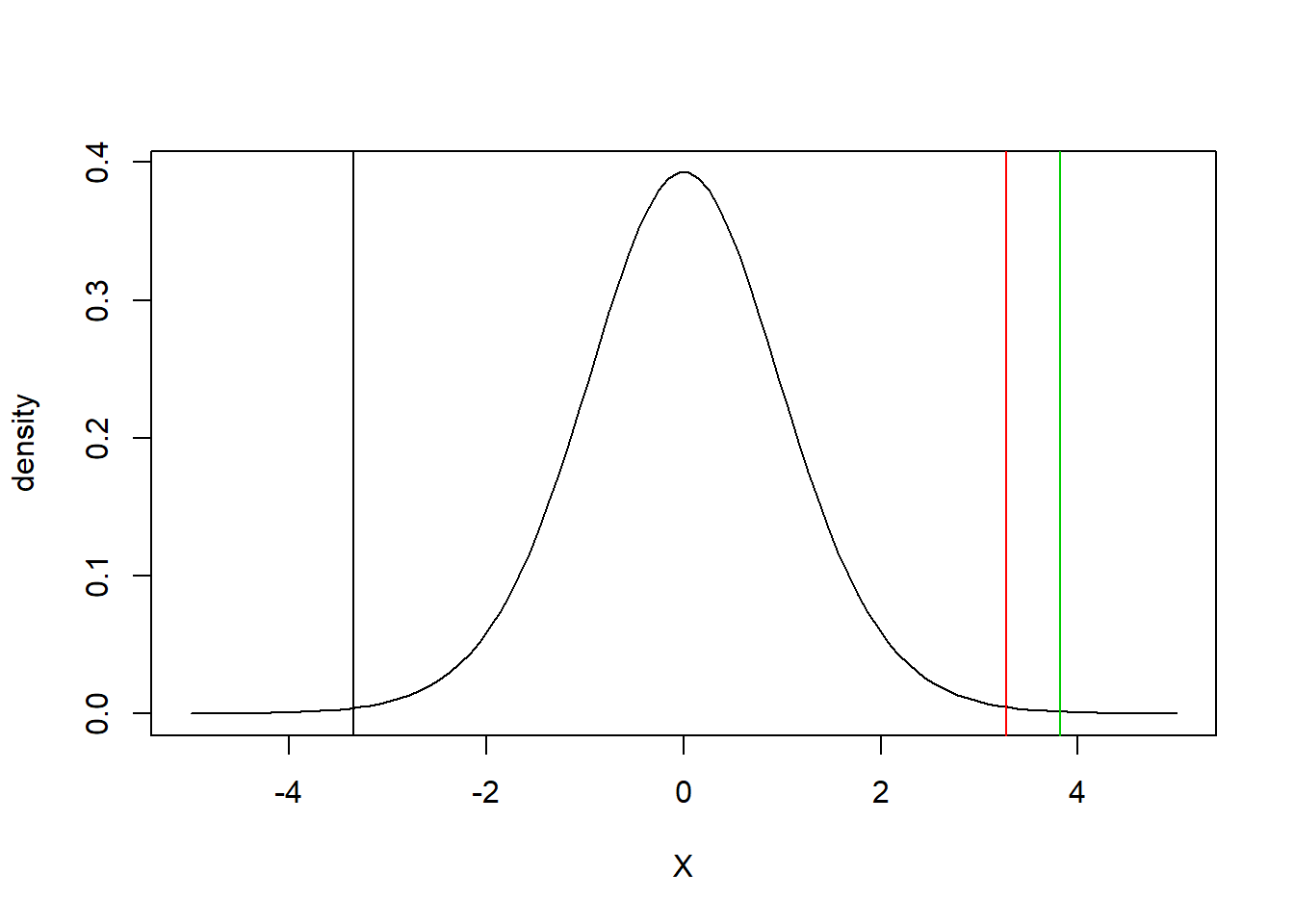

We look at all of the ratings row by row using apply with the cusum function.

cum.probs <- t(apply(P.reverse, 1, function(v) {
    pmin(0.99999, pmax(1e-05, cumsum(v)))
}))
thresholds <- qt(cum.probs, 16)  ##Use Student-t with 16 degrees of freedom
opa <- par(mfrow = c(2, 4))
for (j in 1:nrow(thresholds)) {
    plot(seq(from = -8, to = 8, length = 100), 
        dt(seq(from = -8, to = 8, length = 100), 
            16), type = "l", xlab = "Deviation", 
        ylab = "Density", main = paste("Rating ", 
            rownames(thresholds)[j]))
    abline(v = thresholds[j, ], col = 1:length(thresholds[j, 
        ]))
}
par(opa)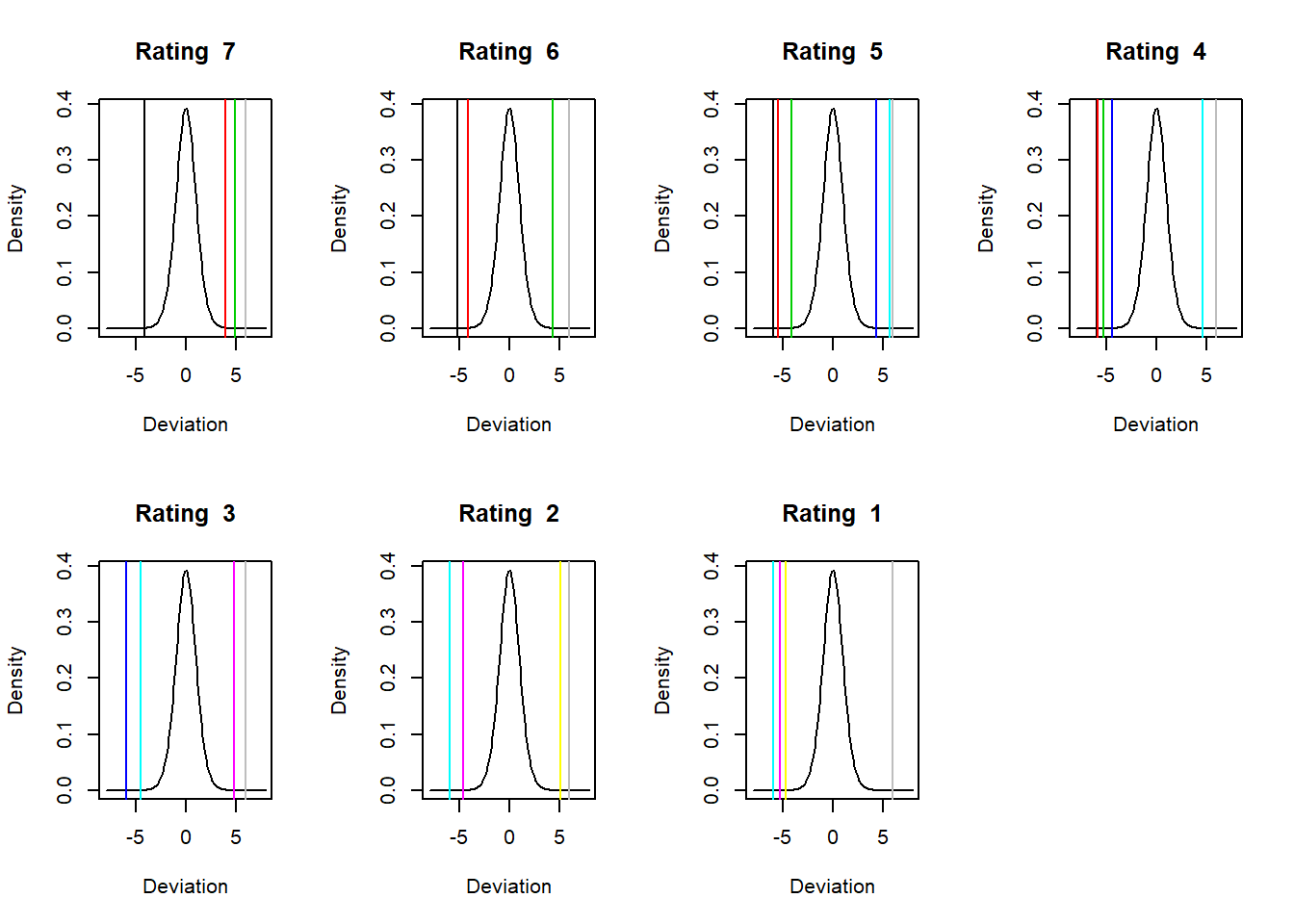

cum.probs is adjusted for 0 and 1 as these might produce NaNs and stop the action. Notice the use of pmin and pmax to perform element by element (parallel minimum and maximum) operations.

This just goes to show it is hard to be rated C. It is the riskiest of all.

7.7 Now for the Finale

We will now use a technique that will can be used with any risk category. The question on the table is: how can we generate a loss distribution for credit risk with so much variation across ratings?

A loss distribution is composed of two elements, frequency and severity.
Frequency asks the question how often and related to that question, how likely.
Severity asks how big a loss.

For operational risk frequency will be modeled by a Poisson distribution with an average arrival rate of any loss above a threshold. Severity will be modeled using Beta, Gamma, Exponential, Weibull, Normal, Log-Normal, Student-t, or extreme value distributions. For credit risk we can model some further components: loss given default (i.e., recovery) and exposure at default for severity, and probability of default for frequency. By the way our transition probabilities are counting distirubtion and have as their basis the Poisson distirbution. We have used both dwelling times AND the computation of hazards with dependent structures to model the transition probabilities.

Let’s look at our top 20 customers by revenue and suppose we have these exposures. Probabilities of default are derived from the transition probabilities we just calculated.

## Specify portfolio characteristics
n.accounts <- 20
exposure.accounts <- c(5, 5, 5, 5, 10, 
    10, 10, 10, 20, 20, 20, 20, 30, 30, 
    30, 30, 40, 40, 40, 40)
probability.accounts <- c(rep(0.1, 10), 
    rep(0.05, 10))

7.8 Enter Laplace

A hugely useful tool for finance and risk is the Laplace transform. Let’s formally define this as the integral (again think cumulative sum).

\[ L(f(t)) = \int_{0}^{\infty}e^{-st}f(t)dt = f(s) \]

where $f(t)$ is a monotonic, piecewise differentiable function, say the cash flow from an asset, or a cumulative density function . To make this “real” for us we can calculate (or look up on a standard table of transforms)

\[ L\{1\} = \int_{0}^{\infty} e^{-st} 1 dt = \frac{1}{s} \]

If $1$ is a cash flow today $t = 0$, then $L\{1\}$ can be interpreted as the present value of $\$1$ at $s$ rate of return in perpetuity. Laplace transforms are thus to a financial economist a present value calculation. They map the time series of cash flows, returns, exposures, into rates of return.

In our context we are trying to meld receivables account exposures, the rate of recovery if a default occurs, and the probability of default we worked so hard to calculate using the Markov chain probabilities.

For our purposes we need to calculate for $m$ exposures the Laplace transform of the sum of losses convolved with probabilities of default:

\[ \sum_{0}^{m} (pd_{i} \,\times lgd_{i} \,\times S_{i}) \]

where $pd$ is the probability of default, $lgd$ is the loss given default, and $S$ is exposure in monetary units. In what follows lgd is typically one minus the recovery rate in the event of default. Here we assume perfect recovery, even our attorney’s fees.

This function effectively computes the cumulative loss given the probability of default, raw account exposures, and the loss given default.

laplace.transform <- function(t, pd, 
    exposure, lgd = rep(1, length(exposure))) {
    output <- rep(NA, length(t))
    for (i in 1:length(t)) output[i] <- exp(sum(log(1 - 
        pd * (1 - exp(-exposure * lgd * 
            t[i])))))
    output
}

7.8.1 It’s technical…

We can evaluate the Laplace Transform at $s = i$ (where $i = sqrt{-1}$, the imaginary number) to produce the loss distribution’s characteristic function. The loss distribution’s characteristic function encapsulates all of the information about loss: means, standard deviations, skewness, kurtosis, quantiles,…, all of it. When we use the characteristic function we can then calculate the Fast Fourier Transform of the loss distribution characteristic function to recover the loss distribution itself. - This is a fast alternative to Monte Carlo simulation. - Note below that we must divide the FFT output by the number of exposures (plus 1 to get the factor of 2 necessary for efficient operation of the FFT).

N <- sum(exposure.accounts) + 1  ## Exposure sum as a multiple of two
t <- 2 * pi * (0:(N - 1))/N  ## Setting up a grid of t's
loss.transform <- laplace.transform(-t * 
    (0+1i), probability.accounts, exposure.accounts)  ## 1i is the imaginary number
loss.fft <- round(Re(fft(loss.transform)), 
    digits = 20)  ## Back to Real numbers
sum(loss.fft)

## [1] 421

loss.probs <- loss.fft/N
loss.probs.1 <- loss.probs[(0:20) * 5 + 
    1]
loss.q <- quantile(loss.probs.1, 0.99)
loss.es <- loss.probs.1[loss.probs.1 > 
    loss.q]
barplot(loss.probs.1, names.arg = paste((0:20) * 
    5))

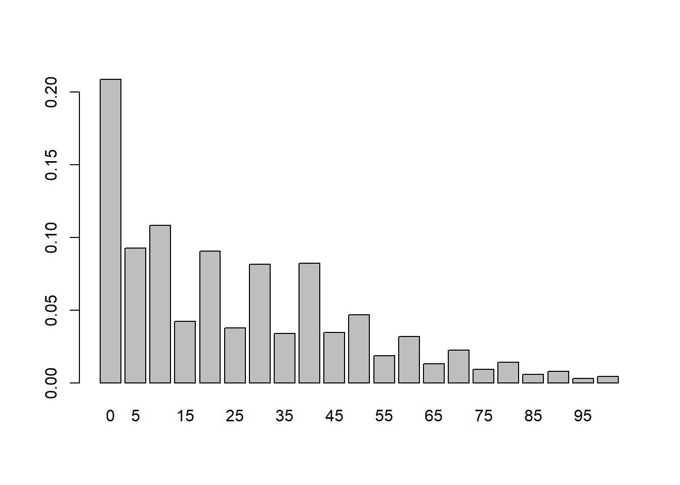
(VaR <- loss.q * N)

##      99% 
## 79.42721

(ES <- loss.es * N)

## [1] 87.89076

We can use this same technique when we try to aggregate across all exposures in the organization. The last two statements using the quantile function calculate the amount of capital we need to cover at least a 1% loss on this portfolio of accounts receivable. The barplot provides a rough and ready histogram of the loss distribution.

7.9 Summary

We covered a lot of credit risk maths: A. Markov, transition probabilities, hazard rates, M. Laplace. We just built a rating model that produced data driven risk thresholds. We used these probabilities to generate an aggregate credit loss distribution.

7.10 Further Reading

Much of the R code in generating hazard-based transition probabilities derives from <

7.11 Practice Laboratory

7.11.1 Practice laboratory #1

7.11.1.1 Problem

7.11.1.2 Questions

7.11.2 Practice laboratory #2

7.11.2.1 Problem

7.11.2.2 Questions

7.12 Project

7.12.1 Background

7.12.2 Data

7.12.3 Workflow

7.12.4 Assessment

We will use the following rubric to assess our performance in producing analytic work product for the decision maker.

The text is laid out cleanly, with clear divisions and transitions between sections and sub-sections. The writing itself is well-organized, free of grammatical and other mechanical errors, divided into complete sentences, logically grouped into paragraphs and sections, and easy to follow from the presumed level of knowledge.
All numerical results or summaries are reported to suitable precision, and with appropriate measures of uncertainty attached when applicable.
All figures and tables shown are relevant to the argument for ultimate conclusions. Figures and tables are easy to read, with informative captions, titles, axis labels and legends, and are placed near the relevant pieces of text.
The code is formatted and organized so that it is easy for others to read and understand. It is indented, commented, and uses meaningful names. It only includes computations which are actually needed to answer the analytical questions, and avoids redundancy. Code borrowed from the notes, from books, or from resources found online is explicitly acknowledged and sourced in the comments. Functions or procedures not directly taken from the notes have accompanying tests which check whether the code does what it is supposed to. All code runs, and the R Markdown file knits to pdf_document output, or other output agreed with the instructor.
Model specifications are described clearly and in appropriate detail. There are clear explanations of how estimating the model helps to answer the analytical questions, and rationales for all modeling choices. If multiple models are compared, they are all clearly described, along with the rationale for considering multiple models, and the reasons for selecting one model over another, or for using multiple models simultaneously.
The actual estimation and simulation of model parameters or estimated functions is technically correct. All calculations based on estimates are clearly explained, and also technically correct. All estimates or derived quantities are accompanied with appropriate measures of uncertainty.
The substantive, analytical questions are all answered as precisely as the data and the model allow. The chain of reasoning from estimation results about the model, or derived quantities, to substantive conclusions is both clear and convincing. Contingent answers (for example, “if X, then Y , but if A, then B, else C”) are likewise described as warranted by the model and data. If uncertainties in the data and model mean the answers to some questions must be imprecise, this too is reflected in the conclusions.
All sources used, whether in conversation, print, online, or otherwise are listed and acknowledged where they used in code, words, pictures, and any other components of the analysis.

Financial Engineering Analytics: A Practice Manual Using R