Chapter 2 Getting Up and Running with R and RStudio

2.1 Understanding R
This document is intended to provide needed background for getting started in R. I recommend reading the entire document before taking any actions. I offer step-by-step instructions for getting started at the end of the document.
R is a language R is a programming language, one particularly well suited to statistical analysis and graphing. As with any language, R has a vocabulary and operates according to certain grammatical rules. Although these rules offer needed structure, they can be inflexible, leading to errors when coding. Good intentions are not enough. That said, as with many languages, you will find there to be some flexibility within that structure. There may be more than one way to accomplish a task. Different packages (user-written functions) may have slightly different command structures. These variations can add to the difficulty in learning R. In the end, though, they are akin to different accents or dialects of the same language.
It is also helpful to keep in mind what it is to learn or know R. Unless you work with R daily, you should not expect to memorize the language. Even then, you will only be able to hold a limited number of functions in your head. Instead, think of knowing R as understanding its basic logic, structure, and grammatical conventions. Beyond that, knowing R means knowing how to marshal available resources, bringing them to bear on the task at hand. This typically involves using resources like this e-book or doing a web search for documentation and/or websites that detail a particular package or function. It is there that you will see the full expanse of arguments and options that you can incorporate into your code.
R is free! (and available for Windows, Macs, and Linux machines) One of the most appealing aspects of R is that it is a free, open source software program. Not only is the software free, so are many of the resources available for learning R. Although there are many useful books for purchase and subscription training sites available, it’s also quite possible to learn R using only free resources. In fact, many R books for purchase are available for free in electronic form.
R operates on the basis of code, not interactive menus and dialogue boxes Unlike SPSS or Stata, R does not offer an interface with a menu system and dialogue boxes. Rather, R is almost entirely code based (imagine Stata, but without the menu/dialogue boxes). Just as Stata has do-files, which operate as scripts of code (and annotations), R has RScripts that serve the same purpose. R also has RMarkdown files, which operate like scripts but can be used to automatically produce documents (html, PDF, or Word) containing the code (optional), any text, and the output of your code.
R and R Studio R is the open source software program that you install on your computer. You can download it from any one of the sites hosting the software. See further below for instructions and links. Its interface is pretty basic and many people prefer not to use it directly (though you will need to install it and do so before installing RStudio). Once installed you won’t actually need to open R, as RStudio will draw upon the program automatically.
RStudio is a free, open source integrated development environment (IDE) that you can install after installing R itself. Instructions and relevant links can be found further below. RStudio’s interface offers four quadrants (the default configuration may differ, but is alterable through Tools – Terminal – Terminal Options – Pane Layout. I’ve also changed the appearance of my RStudio to Modern/Material, giving it a dark background with lighter text. You can choose your own scheme through Tools – Terminal – Terminal Options – Appearance.
- Console – This is the R console (R itself). You can type code in the console directly and it is where statistical output appears.
- Plots/Viewer – This quadrant is where graphs appear. It is also where help pages appear.
- Environment/History – This quadrant shows the objects in your session and has a tab containing your command history. It also has an “import dataset” dropdown/dialogue box that can be used to import datasets from other popular programs.
- Script/Markdown/Dataset – This quadrant keeps track of your open Rscripts, RMarkdown documents, and your datasets. You can type your code in a script and execute it from here.
Although I highly recommend learning to use R through RStudio (which the vast majority of users do), there are some free, open source IDEs that approximate, to some degree, the menu/dialogue box systems that one finds in SPSS and Stata. Once both R and RStudio are installed on your computer, you will only ever need to open RStudio to work with R (as R itself is embedded in RStudio).
RStudio Cloud If you do not want to install R/RStudio on your computer, you can register for a free account on RStudio Cloud, which enables users to bypass the installation process. Instead, users work with RStudio through their browser. The free account does come with some limitations, such as a limit of 15 hours of use per month. Paid options are available.
Building Blocks of the R Language
Objects – R is an object-oriented language, in contrast to Stata’s operation-oriented language. What does this mean? What is an object? Objects are nothing more than sets of information that exist within your R session; they are there to be used, manipulated, edited, and generated. Your data set is an object. Your regression results are an object. Your graph may be an object. You may generate a number of objects in the course of doing a project (e.g., you’ll produce three different objects that correspond to three different regression model results). The objects in your R session will appear in the “Environment” tab of RStudio (see screenshot below where there are two objects – a data set and the results of an OLS regression). Although the object-oriented nature of R seems strange at first, it will come to make sense as you progress in your understanding of R.
You generate objects by using the assignment operator <-. Here is an example that shows the generation of an object comprised of OLS regression results. In this case, I am calling that object ols1 and it is the result of regressing y on x (lm stands for linear model), making use of the dataset called mydata. Tip: a shortcut for creating <- is to push the Alt and - keys at the same time.
ols1 <- lm(y ~ x, data = mydata)Since some of the things (e.g., html or pdf documents) you create will be saved to your working directory, you can find that location by typing:
getwd()Packages – R has a number of functions that are native to the base language, but what makes R attractive to many data scientists and researchers is an expansive ecosystem of user-written packages that offer additional functions and options. For those familiar with Stata, these packages are akin to user-written commands and their ado-files, which enrich the built-in capability of Stata. Just as an ado-file consists of a complex script of code (have you ever looked inside an ado file?), making possible a single line of operation code within Stata, so too do packages make possible complex operations with a single line (or a few lines) of code in R.
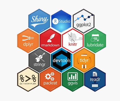
The vast ecosystem of packages for R is both a plus and a minus. On the one hand, there’s almost always a package available for what you want to do. On the other hand, the sheer volume of packages can be daunting. Over time, you will find yourself gravitating toward a manageable number of favored packages (e.g., ggplot2) to accomplish most of what you do.
You can even purchase R package stickers and magnets here, here, and here.
These R packages must be installed. Once installed, you will not need to reinstall a package. You will, however, need to regularly check for any available updates to your collection of packages (see further below). To install a package, type the following in the console of RStudio (note the quotation marks, which are needed when installing):
install.packages("package_name")The code to install all of the packages used in these generic scripts can be found here. Alternatively, I’ve put that same code into a RScript file that can be opened in RStudio.
To make use of a function that is part of an installed package, you must load the package into each new R session. You do this through the library() function. Notice that while you use quotation marks when installing a package (generic code above), you do not need to use them when loading the package into your session.
library(package_name)You will notice in my generic commands pages that I list any needed packages at the top of the page in a series of library() commands. For transparency’s sake, I also include the relevant package in any command that uses a function tied to that package. You will see this at the start of some commands (e.g., package_name::function). It is your choice whether to include package_name:: in your command. Once a package is loaded into your session, you are free to begin your commands with the relevant function.
ggplot2::ggplot(data = mydata, aes(intvar)) + geom_boxplot()

# is equivalent to:

ggplot(data = mydata, aes(intvar)) + geom_boxplot()
To check for and install any updates to your installed packages, in RStudio click on Tools – Check for Package Updates. I do this whenever I remember to do it, often once a week. RStudio will ask if you want to briefly shutdown and reopen before updating, which is a good idea. This will “unload” any active packages, allowing them to be updated. RStudio won’t update a package if it’s currently loaded in a session.
When using a particular package, you’ll find it useful to google its documentation and other helpful wepbages. For any particular function, there can be a lot of possible options – these resources will help you navigate them. Fortunately, you can often get by with the default settings (which you don’t have to type). Here are examples of such resources for a function called plot_model from the sjPlot package.
https://www.rdocumentation.org/packages/sjPlot/versions/2.8.4/topics/plot_model https://mran.revolutionanalytics.com/snapshot/2018-01-06/web/packages/sjPlot/sjPlot.pdf https://strengejacke.github.io/sjPlot/articles/plot_interactions.html
Specifying Your Data in Your Command One of the more unfamiliar features of the R language, for those coming from Stata or SPSS, is the need to specify one’s dataset in each command. This stems from the fact that R can host more than one dataset at a time, making it necessary for the user to indicate which dataset they are using in any particular action. There are two common ways you will see this. First, you may simply see the dataset specified within a command (data = mydata). Second, you may see the dataset specified in front of a variable name, separated by a $. Here are two examples. In the first, I am generating an object consisting of the regression results of y on x, using dataset mydata. In the second, I am declaring a categorical variable (catvar) in my dataset (mydata) to be a factor variable (since I use the same variable name, this results not in a new variable, but an overwrite of the existing variable, or, in this case, merely a reclassification of the variable). Although strange at first, you will quickly get used to specifying your dataset in your commands.
object <- lm(y ~ x, data = mydata)
mydata$catvar <- factor(mydata$catvar)
2.2 Step-by-Step Instructions for Getting Up and Running
If you wish to install R and RStudio on your own computer, follow the instructions below. Here is a short video on how to carryout the installations.
[_]().
Additionally, here is a video demonstrating how to make use of this e-book and the generic RScripts.
[_]()
If you prefer to trial R/RStudio without installing them, you can use RStudio Cloud, which allows users to bypass the need for installation. You simply use RStudio through your browser. It is easy to register for a free account (it does come with some restrictions, such as a maximum of 15 hours of use per month). Here is a short video demonstrating RStudio Cloud.
[_]()
Download and install R. You can find a list of sites that host the R software here. For the sake of narrowing your options, I would recommend using Duke University’s site. Just choose the download appropriate for your operating system. Once installed, there will be no need to actually open up R. It just needs to be installed for RStudio to make use of it.
Download and install the free version of RStudio Desktop. Once installed, open it up RStudio.
Import a dataset. In the Environment pane, you will see an “Import Dataset” button. This will allow you to import datasets from other popular programs (Excel, SPSS, Stata, SAS).
Since this process may draw upon a particular package, RStudio may ask if you want to install the requisite package(s). Do so. You can browse for your desired dataset to import it. Once the desired dataset is selected, allow a moment for the “preview” to load before selecting “Import” at the bottom right of the window. As noted above, you will be referencing this dataset frequently. If it has a lengthy name, you may opt to simplify matters by cloning it and giving it a simple name in the process. Since the generic scripts I offer use “mydata” as the name of the dataset, you might choose to name your cloned dataset that. To do so, in the console window type:
mydata <- whatever_your_imported_dataset_is_calledYou will notice that mydata is now another object in your Environment pane.
Install packages. You can install all of the packages that are used in the generic script all at once. They will only need to be installed this one time, though they may need to be updated from time to time (see further above). The easiest way to install the packages is to download an RScript I created with the requisite code. Once downloaded, select File – Open File – RScript_to_install_packages. Once the RScript opens, highlight all the lines of code and then select “run” near the top right of the RScript. It may take a few minutes to install all of the packages.
Use a generic script page to guide your analysis. Depending on what kind of analysis you need to run, you can draw upon any of the generic script pages found here. As noted above, I HIGHLY recommend that you take the time to type the commands in rather than simply copy/paste them.
The exercise of manually entering the commands is a key part of learning the code. Note that any text in italics should be changed out (e.g., catvar should be replaced by your categorical variable’s name). If you make a typing error and get an error message, rather than retyping the entire command, you can use the up arrow key to pull up your most recent command and edit it from there. You can type the code one command at a time into the Console pane, or you can start a new RScript and type all of your code there, running line(s) as desired.