5 Tutorial 5: Data management with tidyverse
After working through Tutorial 5, you’ll…
- know how to inspect and change data
For this tutorial, we’ll again use the data set “data_fictional_survey.csv” (via Moodle/Data for R). The data set has already been introduced and explained, so I won’t go into detail here.
5.1 What is the tidyverse?
The so-called tidyverse is a popular collection of different R packages especially useful and accessible for R “beginners”4.
These include…
tibble: creating data structures like tibbles, which is an enhanced type of data framereadr,haven,readxl: reading data (e.g. readr for CSV, haven for SPSS, Stata and SAS, readxl for Excel)tidyr,dplyr: data transformation, modification, and summary statisticsstringr,forcats,lubridate: create special, powerful object types (e.g.stringrfor working with text objects,forcatsfor factors,lubridatefor time data)purrr: programming with Rggplot2: graphing/charting
The most frequently used packages of the tidyverse can be installed and activated like so (you may have to do so for less frequently used packages separately):
In the following, I’ll give you a short introduction into the tidyverse (especially dplyr for data wrangling), but not an overall introduction. For more detailed sources on this, see
5.2 Tibbles for our data
The tidyverse also comes with a specific data structure: tibbles.
Usually, you can forget all about vectors, lists etc. - just save your data as a tibble, which follows three rules:
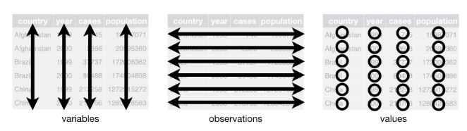
- Columns: Every column is one variable.
- Rows: Every row is one observation.
- Cells: Every cell contains one single value.
Image: Structure of Tibbles Source: R for Data Science
Let’s have a look at our survey data in tibble format:
## # A tibble: 20 x 6
##    name         age date       outlet outlet_use outlet_trust
##    <chr>      <int> <chr>      <chr>       <int>        <int>
##  1 Alexandra     20 09.09.2021 TV              2            5
##  2 Alex          25 08.09.2021 Online          3            5
##  3 Maximilian    29 09.09.2021 Print           4            1
##  4 Moritz        22 06.09.2021 TV              2            2
##  5 Vanessa       25 07.09.2021 Online          1            3
##  6 Andrea        26 09.09.2021 Online          3            4
##  7 Fabienne      26 09.09.2021 TV              3            2
##  8 Fabio         27 09.09.2021 Online          0            1
##  9 Magdalena      8 08.09.2021 Online          1            4
## 10 Tim           26 07.09.2021 TV             NA            2
## 11 Alex          27 09.09.2021 Online         NA            2
## 12 Tobias        26 07.09.2021 Online          2            2
## 13 Michael       25 09.09.2021 Online          3            2
## 14 Sabrina       27 08.09.2021 Online          1            2
## 15 Valentin      29 09.09.2021 TV              1            5
## 16 Tristan       26 09.09.2021 TV              2            5
## 17 Martin        21 09.09.2021 Online          1            2
## 18 Anna          23 08.09.2021 TV              3            3
## 19 Andreas       24 09.09.2021 TV              2            5
## 20 Florian       26 09.09.2021 Online          1            5
5.3 Pipes for our functions
Another nice feature of the tidyverse is the pipe operator, an element of the dplyr package within the tidyverse. dplyr is one of the most popular packages belonging to the tidyverse. It contains a lot of really helpful functions for data data transformation. For help, see this useful cheat sheet on dplyr.
For data management, dplyr relies on the pipe operator: %>%. The %>% operator allows functions to be applied sequentially to the same object, making it easy to understand transformations step-by-step.
Here, we always call the source object first and then add each transformation step separated by the %>% operator. The pipe operator %>% takes a certain object which is then passed over to one or several functions to its right.
Remember the command from before? That is exactly what we did here:
We (1) take the object survey, we then (2) push it into the pipe %>% and we (3) then use the as_tibble() command to transform the object:
Remember: If you want to save the result, you have to save the resulting object, for example like so:
5.4 Data management with dplyr
dplyr comes with five main functions:
select(): select variables column by column, i.e. pick columns / variables by their namesfilter(): filter observations row by row, i.e. pick observations by their valuesarrange(): sort / reorder data in ascending or descending ordermutate(): calculate new variables or transform existing onessummarize(): summarize variables (e.g. mean, standard deviation, etc.), best combined withgroup_by()
5.4.1 Select specific variables
You will frequently encounter large data sets including hundreds of variables. The first problem in this scenario is narrowing down the variables you are truly interested in. select() helps you to easily choose a suitable subset of variables. In this selection process, the name of the data frame is the source object, followed by the pipe %>% operator. The expression that selects the columns that you are interested in comes after that.
Using the survey, we may for example want to only include specific variables for a reduced data set.
Let’s assume you want to reduce the object survey to the variables name and age using select:
##          name age
## 1   Alexandra  20
## 2        Alex  25
## 3  Maximilian  29
## 4      Moritz  22
## 5     Vanessa  25
## 6      Andrea  26
## 7    Fabienne  26
## 8       Fabio  27
## 9   Magdalena   8
## 10        Tim  26
## 11       Alex  27
## 12     Tobias  26
## 13    Michael  25
## 14    Sabrina  27
## 15   Valentin  29
## 16    Tristan  26
## 17     Martin  21
## 18       Anna  23
## 19    Andreas  24
## 20    Florian  26
You can also delete columns by making a reverse selection with the - symbol. This means that you select all columns except the one whose name you specify.
##    age       date outlet outlet_use outlet_trust
## 1   20 09.09.2021     TV          2            5
## 2   25 08.09.2021 Online          3            5
## 3   29 09.09.2021  Print          4            1
## 4   22 06.09.2021     TV          2            2
## 5   25 07.09.2021 Online          1            3
## 6   26 09.09.2021 Online          3            4
## 7   26 09.09.2021     TV          3            2
## 8   27 09.09.2021 Online          0            1
## 9    8 08.09.2021 Online          1            4
## 10  26 07.09.2021     TV         NA            2
## 11  27 09.09.2021 Online         NA            2
## 12  26 07.09.2021 Online          2            2
## 13  25 09.09.2021 Online          3            2
## 14  27 08.09.2021 Online          1            2
## 15  29 09.09.2021     TV          1            5
## 16  26 09.09.2021     TV          2            5
## 17  21 09.09.2021 Online          1            2
## 18  23 08.09.2021     TV          3            3
## 19  24 09.09.2021     TV          2            5
## 20  26 09.09.2021 Online          1            5
5.5 Select specific observations
filter() divides observations into groups depending on their values. The name of the data frame is the source object, followed by the pipe %>% operator. Then follow the expressions that filter the data.
Let’s say we want to include include those observations from the object survey where respondents said that they were older than 21 years via filter().
## 'data.frame':    20 obs. of  6 variables:
##  $ name        : chr  "Alexandra" "Alex" "Maximilian" "Moritz" ...
##  $ age         : int  20 25 29 22 25 26 26 27 8 26 ...
##  $ date        : chr  "09.09.2021" "08.09.2021" "09.09.2021" "06.09.2021" ...
##  $ outlet      : chr  "TV" "Online" "Print" "TV" ...
##  $ outlet_use  : int  2 3 4 2 1 3 3 0 1 NA ...
## $ outlet_trust: int 5 5 1 2 3 4 2 1 4 2 ...## 'data.frame': 17 obs. of 6 variables:
## $ name : chr "Alex" "Maximilian" "Moritz" "Vanessa" ...
## $ age : int 25 29 22 25 26 26 27 26 27 26 ...
## $ date : chr "08.09.2021" "09.09.2021" "06.09.2021" "07.09.2021" ...
## $ outlet : chr "Online" "Print" "TV" "Online" ...
## $ outlet_use : int 3 4 2 1 3 3 0 NA NA 2 ...
## $ outlet_trust: int 5 1 2 3 4 2 1 2 2 2 ...We can even build more complicated filters: Let’s only include respondents older than 21 years and say they mainly use the TV:
## 'data.frame':    20 obs. of  6 variables:
##  $ name        : chr  "Alexandra" "Alex" "Maximilian" "Moritz" ...
##  $ age         : int  20 25 29 22 25 26 26 27 8 26 ...
##  $ date        : chr  "09.09.2021" "08.09.2021" "09.09.2021" "06.09.2021" ...
##  $ outlet      : chr  "TV" "Online" "Print" "TV" ...
##  $ outlet_use  : int  2 3 4 2 1 3 3 0 1 NA ...
## $ outlet_trust: int 5 5 1 2 3 4 2 1 4 2 ...## 'data.frame': 7 obs. of 6 variables:
## $ name : chr "Moritz" "Fabienne" "Tim" "Valentin" ...
## $ age : int 22 26 26 29 26 23 24
## $ date : chr "06.09.2021" "09.09.2021" "07.09.2021" "09.09.2021" ...
## $ outlet : chr "TV" "TV" "TV" "TV" ...
## $ outlet_use : int 2 3 NA 1 2 3 2
## $ outlet_trust: int 2 2 2 5 5 3 55.6 Arrange data
arrange() changes the order of observations (either ascending or descending). By default, arrange() will sort in ascending order, i.e. from 1:100 (numeric vector) and from A:Z (character vector). arrange() must always be applied to at least one column that is to be sorted.
Let’s sort our respondents by name:
##          name age       date outlet outlet_use outlet_trust
## 1        Alex  25 08.09.2021 Online          3            5
## 2        Alex  27 09.09.2021 Online         NA            2
## 3   Alexandra  20 09.09.2021     TV          2            5
## 4      Andrea  26 09.09.2021 Online          3            4
## 5     Andreas  24 09.09.2021     TV          2            5
## 6        Anna  23 08.09.2021     TV          3            3
## 7    Fabienne  26 09.09.2021     TV          3            2
## 8       Fabio  27 09.09.2021 Online          0            1
## 9     Florian  26 09.09.2021 Online          1            5
## 10  Magdalena   8 08.09.2021 Online          1            4
## 11     Martin  21 09.09.2021 Online          1            2
## 12 Maximilian  29 09.09.2021  Print          4            1
## 13    Michael  25 09.09.2021 Online          3            2
## 14     Moritz  22 06.09.2021     TV          2            2
## 15    Sabrina  27 08.09.2021 Online          1            2
## 16        Tim  26 07.09.2021     TV         NA            2
## 17     Tobias  26 07.09.2021 Online          2            2
## 18    Tristan  26 09.09.2021     TV          2            5
## 19   Valentin  29 09.09.2021     TV          1            5
## 20    Vanessa  25 07.09.2021 Online          1            3
5.7 Change values
Often you want to add new columns to a data set, e.g. when you calculate new variables or when you want to store re-coded values of other variables. With mutate(), new columns will be added to the end of you data frame while replace() replaces existing values in an existing variable.
For example, we can create a new variable that indicates whether respondents most use “traditional news media” (TV, Print) or “online media” (Online) like so:
survey %>%
  mutate(traditional = "yes",
         traditional = replace(traditional,
                               outlet == "Online",
                               "no")) %>%
  head()
## name age date outlet outlet_use outlet_trust traditional
## 1 Alexandra 20 09.09.2021 TV 2 5 yes
## 2 Alex 25 08.09.2021 Online 3 5 no
## 3 Maximilian 29 09.09.2021 Print 4 1 yes
## 4 Moritz 22 06.09.2021 TV 2 2 yes
## 5 Vanessa 25 07.09.2021 Online 1 3 no
## 6 Andrea 26 09.09.2021 Online 3 4 noAnother example: Let’s say that we want to transform the variable outlet_trust in the object survey.
Remember: The variable indicates how much each student trusts a specific media outlet described in the variable outlet (from 1 = not at all to 5 = very much).
Instead of numeric values ranging from 1 to 5, we want to create a new variable named which should include:
- “low trust” instead of the numeric values 1 and 2
- “medium trust” instead of the numeric value 3
- “high trust” instead of the numeric values 4 and 5
We use mutate() and replace()` to create new variables based on our existing data.
#get object
survey %>%
  #create empty variable
  mutate(outlet_trust_new = NA) %>%

#transform trust scores
  mutate(outlet_trust_new = replace(outlet_trust_new,
                                    outlet_trust<=2,
                                    "low trust"),

         outlet_trust_new = replace(outlet_trust_new,
                                    outlet_trust==3,
                                    "medium trust"),

         outlet_trust_new = replace(outlet_trust_new,
                                    outlet_trust>=4,
                                    "high trust")) %>%
  head()
## name age date outlet outlet_use outlet_trust outlet_trust_new
## 1 Alexandra 20 09.09.2021 TV 2 5 high trust
## 2 Alex 25 08.09.2021 Online 3 5 high trust
## 3 Maximilian 29 09.09.2021 Print 4 1 low trust
## 4 Moritz 22 06.09.2021 TV 2 2 low trust
## 5 Vanessa 25 07.09.2021 Online 1 3 medium trust
## 6 Andrea 26 09.09.2021 Online 3 4 high trust5.8 Summarize values
Lastly, summarize() function collapses a data frame into a single row that shows you summary statistics about your variables.
We can, for example, calculate the average age of respondents like so:
##   mean_age
## 1     24.4
The summarize() function grows especially powerful when it is combined with group_by to display summary statistics for groups.
We can, for example, calculate the average age of respondents dependent on which outlet they say the use most:
## # A tibble: 3 x 2
##   outlet mean_age
##   <chr>     <dbl>
## 1 Online     23.9
## 2 Print      29
## 3 TV         24.5
💡 Take Aways
- pipe data for subsequent transformation:
%>% - select variables:
select() - select observations:
filter() - arrange data:
arrange() - transform values:
mutate(),replace() - summarize values:
summarize(),group()
📚 More tutorials on this
You still have questions? The following tutorials & papers can help you with that:
📌 Test your knowledge
You’ve worked through all the material of Tutorial 5? Let’s see it - the following tasks will test your knowledge.
Since it is almost Halloween season, we’ll work with a data set from fivethirthyeight on The Ultimate Halloween Candy Power Ranking.
In short, the data contains an online survey in which participants were asked to choose their favorite out of two different candy types. The data is accessible via a Creative Commons Attribution 4.0 International License here. You’ll have to copy the data into a “.txt” file. Else, you can also download the data from Moodle/Data for R (file called data_halloween.txt).
The data includes a range of variables, including
- the name of each candy bar:
competitorname - whether the candy bar contains chocolate:
chocolate - whether the candy bar contains fruit flavor:
fruity - whether the candy bar contains caramel:
caramel - the unit price percentile the candy bar is in compared to the rest of the set:
pricepercent
Task 5.1
Read the data set into R. Writing the corresponding R code, find out
- how many observations and how many variables the data set contains.
Task 5.2
Writing the corresponding R code, find out
- how many candy bars contain chocolate.
- how many candy bars contain fruit flavor.
Task 5.3
Writing the corresponding R code, find out
- the name(s) of candy bars containing both chocolate and fruit flavor.
Task 5.4
Create a new data frame called data_new. Writing the corresponding R code,
- reduce the data set only observations containing chocolate but not caramel. The data set should also only include the variables
competitornameandpricepercent. - round the variable
pricepercentto two decimals. - sort the data by
pricepercentin descending order, i.e., make sure that candy bars with the highest price are on top of the data frame and those with the lowest price on the bottom.
The corresponding data frame should look like this:
##                 competitorname pricepercent
## 1              Nestle Smarties         0.98
## 2            Hershey's Krackel         0.92
## 3     Hershey's Milk Chocolate         0.92
## 4       Hershey's Special Dark         0.92
## 5                  Mr Good Bar         0.92
## 6                       Mounds         0.86
## 7                     Whoppers         0.85
## 8                   Almond Joy         0.77
## 9          Nestle Butterfinger         0.77
## 10               Nestle Crunch         0.77
## 11         Peanut butter M&M's         0.65
## 12                       M&M's         0.65
## 13                 Peanut M&Ms         0.65
## 14   Reese's Peanut Butter cup         0.65
## 15              Reese's pieces         0.65
## 16 Reese's stuffed with pieces         0.65
## 17                3 Musketeers         0.51
## 18             Charleston Chew         0.51
## 19                Junior Mints         0.51
## 20                     Kit Kat         0.51
## 21        Tootsie Roll Juniors         0.51
## 22                 Tootsie Pop         0.32
## 23     Tootsie Roll Snack Bars         0.32
## 24          Reese's Miniatures         0.28
## 25            Hershey's Kisses         0.09
## 26                     Sixlets         0.08
## 27        Tootsie Roll Midgies         0.01
This is where you’ll find solutions for Tutorial 5. Let’s keep going: Tutorial 6: Intro to Scraping.
Though I never met anyone who “finished” R, so remember that we are all beginners in R - or that we are all learning R, but are at different stages of doing so.↩︎