2 Tutorial 2: What to do where in R Studio
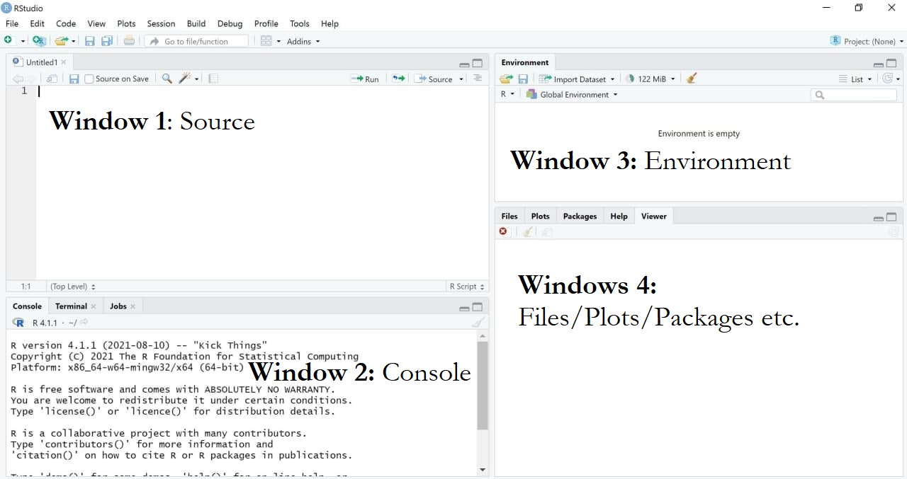
As mentioned, R studio is a graphical interface which facilitates programming with R. It contains up to four main windows, which allow for different things:
Window 1 (Source): Writing your own code. Important: When first installing R/R Studio and opening R studio, you may not see this window right away. In this case, simply open it by clicking on File/New File/R Script.
Window 2 (Console): Executing your own code.
Window 3 (Environment): Inspecting objects
Window 4 (Files/Plots/Packages): Visualizing data, searching for help, updating packages etc.
Image: Four main windows in R
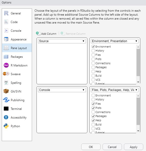
Please note that the specific set-up of your R Studio may look different (the order of windows may vary and so may the windows’ names). I have made the experience that having these four windows open works best for me. This may be different for you. If you want to modify the appearance of your R Studio, simply choose “Tools/Global Options/Pane Layout”.
Image: Changing the Layout
In the options menu, you can perform various cool customizations, such as enabling rainbow parentheses via “Tools/Global Options/Code/Display”. With this feature, a starting parenthesis will be displayed in the same color as its corresponding closing parenthesis.
2.1 Source: Write your own code
Using the window “Source”, you’ll write your own code to execute whichever task you want R to fulfill.
2.1.1 Write Code
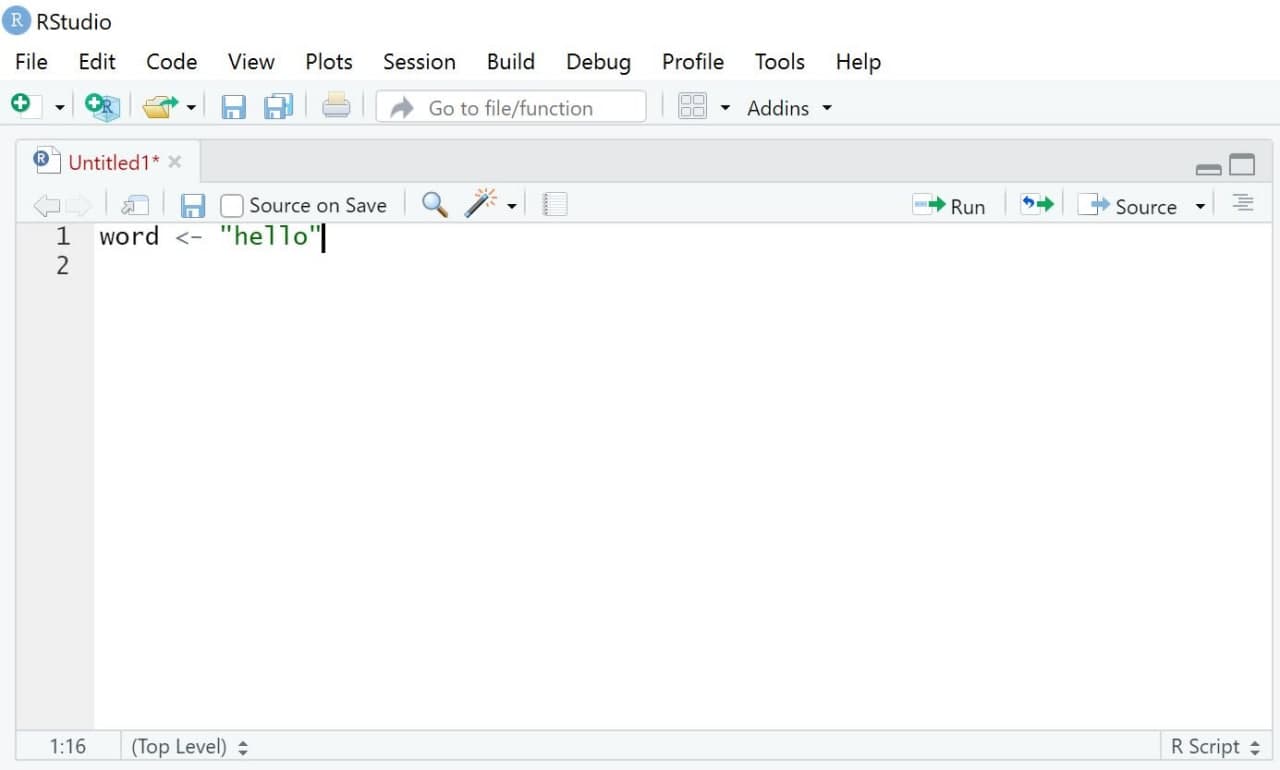
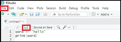
Let’s start with an easy example: Assume you simply want R to print the word “hello”. In this case, you would first write a simple command that assigns the word “hello” to an object called word. The assigment of values to named objects is done via either the operator <- or the operator =. The left side of that command contains the object that should be created; its right side the values that should be assigned to this object.
In short, this command tells R to assign the world “hello” to an object called word.
Image: “Source”
2.1.2 Annotate Code
Another helpful aspect of R is that you can comment your own code. Oftentimes, this is very helpful for understanding your code later (if you write several hundred lines of codes, you may not remember their exact meaning months later).
Comments or notes can be made via hashtags #. Anything following a hashtag will not be considered code by R but be ignored instead.
A pretty cool feature is that you can use hashtags to structure your word in blocks - think of them like “chapter headings” in Word or similar.
If you add four hashtags before and after a heading ####, R will create a heading (see below). You can use these to jump from specific code to the next. This is especially useful if you have long sections of code, as it gives you a better overview and structure.
Image: Structuring Code

2.1.3 Execute Code
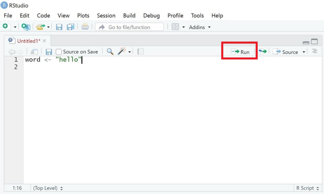
We now want to execute our code. Doing so is simple:
- Mark the parts of the code you want to run (for instance, single rows of code or blocks of code across several rows)
- Either press Run (see upper right side of the same window) or press Alt + Enter. On Mac OS X, hold the command key and press return instead.
R should now execute exactly those lines of codes that you marked (hereby creating the object word). If you haven’t marked any specific code, all lines of code will be executed.
Image: Executing Code
Some commands run for a longer time - and you may realize while they are running that the code still contains an error. In this case, you may want to stop R in executing the command. If you want to do this manually, you can use the stop button in the window “Console” (only visible while R is executing code).
Image: Interrupting R
Else, you can use the menu via Session / Interrupt R.
2.1.4 Save Code
A great feature of R is that it makes analyses easily reproducible - given that you save your code. When reopening R Studio and your script, you can simply “rerun” the code with one click and your analysis will be reproduced.
To save code, you have two options:
- Choose the menu option File/Save as. Important: Code needs to be saved with the ending “.R”.
- Chose the Save-button in the source window and save your code in the correct format, for instance as “MyCode.R”
2.2 Console: Print results
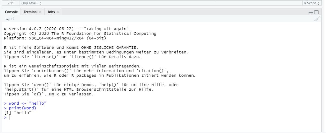
Results of executing code are printed in a second window called “Console”, which includes the code you ran and the object you may have called when doing so.
Previously, we defined an object called word, which consists of the single word “hello”. Thus, R prints our code as well as objects called when running this code (here, the object word) in the console.
## [1] "hello"Image: Window “Console”
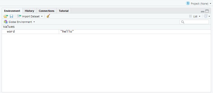
2.3 Environment: Overview of objects
The third window is called “Environment”1. This windows displays all the objects currently existing - in our case, only the object “word”. As soon as you start creating more objects, this environment will fill up.
If you’re an SPSS user, this window is very similar to what is called the Datenansicht / Data overview in SPSS. However, the R version of this is much more flexible, given that our environment can contain several data sets, for example, at the same time.
Image: Window “Environment”
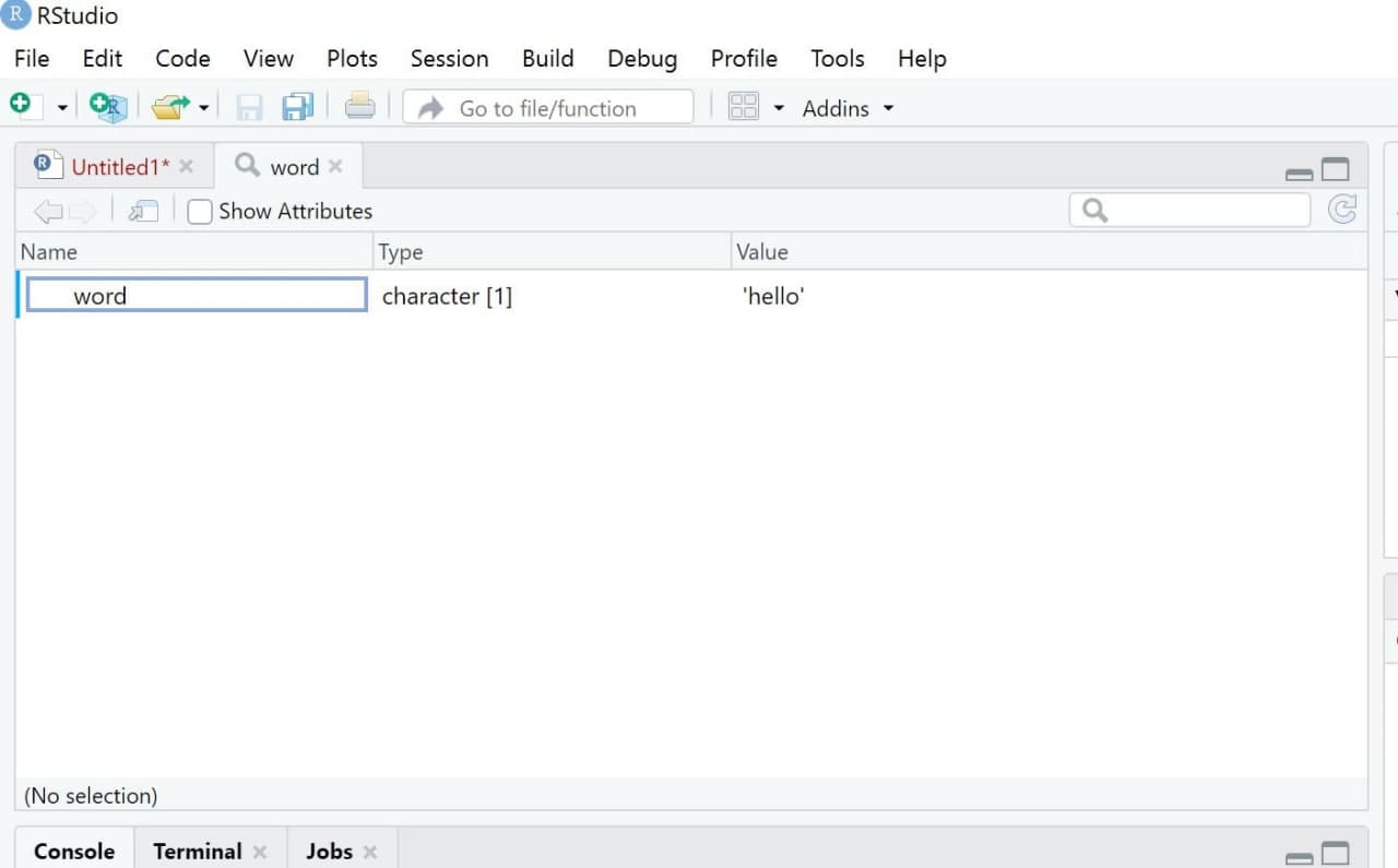
It is important to know that we can visually inspect any object using the View() command (with a new tab then opening in the “Source” window). While this may not seem particularly useful at the moment, it becomes immensely helpful when working with larger datasets that have multiple observations and variables.
Image: Window “View”
2.4 Plots/Help/Packages: Do everything else
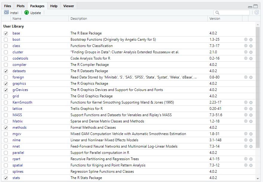
Lastly, the standard R Studio interface contains a fourth window (if you opted for this layout). In my case, the window contains several sub-sections called “Files”, “Plots”, or “Packages” among others. You’ll understand their specific functions later - the window can, for instance, be used to plot/visualize results or see which packages are currently loaded.
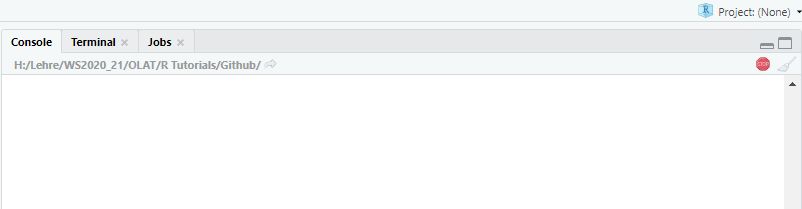
Image: Window “Files/Plots/Packages”
2.5 Packages
While Base R already includes many helpful functions, you may at times need other, additional functions. For instance, if we want to use R for web scraping we’ll need to use specific packages including additional functions.
Packages are collections of topic-specific functions that extend the functions implemented in Base-R.
In the spirit of “open science”, anyone can write and publish these additional functions and related packages and anyone can also access the code used to do so.
You’ll find a list of all of R packages here. In this seminar, we’ll for instance use packages like dplyr for advanced data management.
2.5.1 Install packages
To use a package, you have to install it first. Let’s say you’re interested in using the package Quanteda. Using the command install.packages(), you can install the package on your computer. You’ll have to give the function the name of the package you are interested in installing.
Now the package has been installed on your computer and is accessible locally. We only have to use install.packages() for any package once. Afterwards, the only thing you’ll have to do after open R is to activate the already installed package - which we’ll learn next.
2.5.2 Activate packages
Before we are able to use a package, we need to activate it in each session via the library() command. Again, you’ll have to give R the name of the package you want to activate:
Else, you can also use the name of the package followed by two colons :: to activate a package directly before calling one of its function. For instance, I do not need use to activate the quanteda package using the library() command to use the function tokens() if I use the following command:
2.5.3 Get info about packages
The package is installed and activated - but how can we use it? To get an overview of functions included in a given package, you can consult its corresponding “reference manual” (overview document containing all of a package’s functions) or, if available, its “vignette” (tutorials on how to use selected functions for the corresponding package) provided by a package’s author on a website called “CRAN”.
The easiest way to finding these manuals/vignettes is Google: Simply google CRAN Quanteda, for instance, and you’ll be guided to the following website.
The first paragraph gives you an overview of aspects for which this package may be useful. The second area links to the reference manual and the vignette. You can, for instance, check out the reference manual to get an idea of the many functions the quanteda package contains.
💡 Take-Aways
- Window “Source”: used to write/execute code in R
- Window “Console”: used to return results of executed code
- Window “Environment”: used to inspect objects on which to use functions
- Window “Files/Plots/Packages etc.”: used for additional functions, for instance visualizations/searching for help/activating or updating packages
- Packages: collections of topic-specific functions that extend the functions implemented in Base-R.
📚 More tutorials on this
You still have questions? The following tutorials & papers can help you with that:
- YaRrr! The Pirate’s Guide to R by N.D.Phillips, Tutorial 2
- Computational Methods in der politischen Kommunikationsforschung by J. Unkel, Tutorial 1
- Continuing education in R by Lara Kobilke, Tutorial 2
- SICSS Boot Camp by C. Bail, Video 1
- wegweisR by M. Haim, Video 1
- R Cookbook by Long et al., Tutorial 1
Let’s keep going: Tutorial 3: Workflow in R
again, this only applies for the way I set up my R Studio. You can change this via “Tools/Global Options/Pane Layout”↩︎