3 Tutorial 3: Workflow in R
Tutorial 3 will help you to understand the basic workflow when working with R and R Studio - independent of whether you want to calculate a regression model, do an automated content analysis, or visualize results of an analysis.
After working through Tutorial 3, you’ll…
- understand the basic work flow in R.
- theoretically know how to now run code in R.
3.1 Define your working directory
The first step of any type of analysis is to define your working directory. You may wonder: What’s that?
Your working directory is the folder from which data can be imported into R or to which you can export and save data created with R.
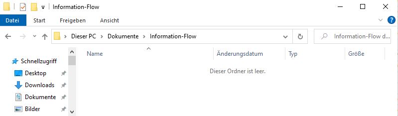
Create a folder that you want to use as your working directory for this tutorial (or use an existing one, that also works). For this tutorial, I created a folder called “Information-Flow”.
Image: Working Directory on Windows
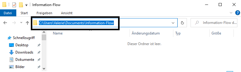
Go to that folder and copy the path to it2:
Image: Copy Path to Working Directory on Windows
On Mac, you go to a document in your folder and click on it (right click). An options menu opens and you can copy the folder path.
Now you know where this working directory is located - but R should know, too! Telling R from which folder to import data or where to export data to is also called setting your working directory. We call a function called setwd() (you guessed right: short for “setting you working directory”) which allows us to do exactly that.
Important: The way this working directory is set differs between Windows- and Mac-Operating Systems.
Windows: The dashes need to be pointing towards the right direction (if you simply copy the path to the folder, you may need to replace these signs “\” with “/”)
Mac: You may need to add a “/” at the beginning like so:
If you have forgotten where you set your working directory, you can also ask R about the path of your current working directory with getwd():
## [1] "C:/Users/vhase/Documents/Information-Flow"3.2 Activate packages
In a next step, you would activate packages you need for your analyses (and newly install those that you have not yet installed).
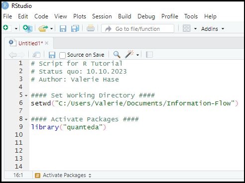
For example, you could define your working directory and activate relevant packages like so:
Define Working Directory & Activate Packages
3.3 Import data (potentially)
Oftentimes, you may want to import data that you saved outside of R into R. This is not always necessary, but I will quickly show you how this works.
3.3.1 Read in external files
Here, we’ll use the Excel file “data_fictional_survey.csv” (via Moodle/Data for R).
One of the most frequently encountered external data types you’ll have to get into R are comma-separated values files, or short, CSV files. You may know CSV files from Excel - oftentimes, such data consists of observations (in rows) and variables (in columns). Values are separated by a separator (oftentimes a comma or a semicolon, depending on your data).
Information on the data set
The data set consists of data that is completely made up - a survey with 20 fictional students in a fictional seminar. We only use this data here so you can understand how to import data.
- Each row contains the answer for a single student.
- Each column contains all values given by students for a single variable.
The variables included here are:
- name: the name of each student
- age: the age of each student (in years)
- date: the date on which each student was surveyed (in YYYY-MM-DD)
- outlet: the type of media outlet each student’s mainly uses to get information
- outlet_use: the time each student uses this media outlet daily (in hours)
- outlet_trust: how much each student trusts this media outlet (from 1 = not at all to 5 = very much)
We’ll read in the file with read.csv(). Here, we specify where to find the data file with the argument x as well as that the first row contains variable names with the argument header = TRUE.
What does this command do? Let’s see:
Image: Help for the read.csv2 function
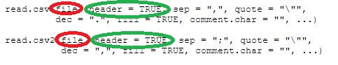
The read.csv2() function is part of the utils package. To read in CSV files, two different functions exist:
read.csv()reads in CSV files where values are comma separatedread.csv2()reads in CSV files where values are semicolon separated
Other than that, both functions work the same way and consist of the same arguments:
file: Here, you need to identify the name of the CSV files that should be read in (including the file extension, here .csv). The file should be located in your working directory, otherwise R will not be able to identify it:file = "data_fictional_survey.csv"header: This argument specifies whether or not the first row of the CSV file contains the name of variables. It is automatically set to true - thus, if our data wouldn’t contain the name of each variable in its first row, we would need to set this argument toFALSE. In our case, we could either ignore this argument (since it is automatically set toTRUE) or actively set it toTRUE. Both leads to the same result.
Important: R differentiates between necessary (marked in red) and obligatory (marked in green) arguments.
Arguments where no default value is given (i.e., those without a =) are necessary. That means you have to specify it once you call the function by passing respective values to the function. For instance, you cannot read in a CSV file without specifying the argument file - R would not even know which file to read in in that case.
However, arguments were are default value is given can be ignored. If you do not specify values for these arguments yourself, R will simply take the default value. For instance, the read.csv2() function will automatically use the first row of a CSV file as column names, unless you actively set the argument header to FALSE.
Another important thing to know is that you can specify arguments in functions in two ways:
- explicitly by name, for instance by setting `file* equal to data_fictional_survey.csv
- implicitly by order, for instance by passing data_fictional_survey.csv as the first argument to the
read.csv2()function
In fact, the following two commands will give the exact same results:
3.3.2 Load existing working spaces
If you saved results in a previous session, you can now also easily import them in a new session via the load() command, you can import working spaces into a new R session.
Here, we’ll use the working space that includes the survey data from above. Download the file “working-space-tutorial2.RDATA” (via Moodle/Data for R).
To see that this actually work, delete all objects in your current working environment. By specifying an empty lists of objects, ls(), as the element to be deleted via rm(), all objects get deleted:
Your working environment should now be empty.
Using the load() function, import “working-space-tutorial2.RDATA” into R.
3.4 Save code & results
Of course, you would usually write more code & conduct more analyses in R than “merely” loading existing data - but that is something we will learn in the next tutorials.
For now, we do two things: we save our code and our results.
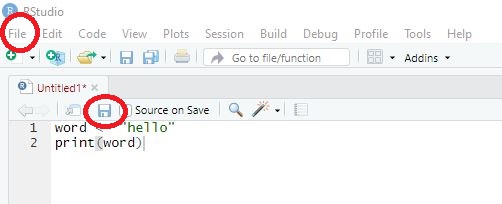
3.4.1 Save your code
A great feature of R is that it makes analyses easily reproducible - given that you save your code. When reopening R Studio and you script, you can simply “rerun” the code with one click and your analysis will be reproduced.
To save code, you have two options:
- Choose the menu option File/Save as. Important: Code needs to be saved with the ending “.R”.
- Chose the Save-button in the source window and save your code in the correct format, for instance as “MyCode.R”.
Image: Saving code
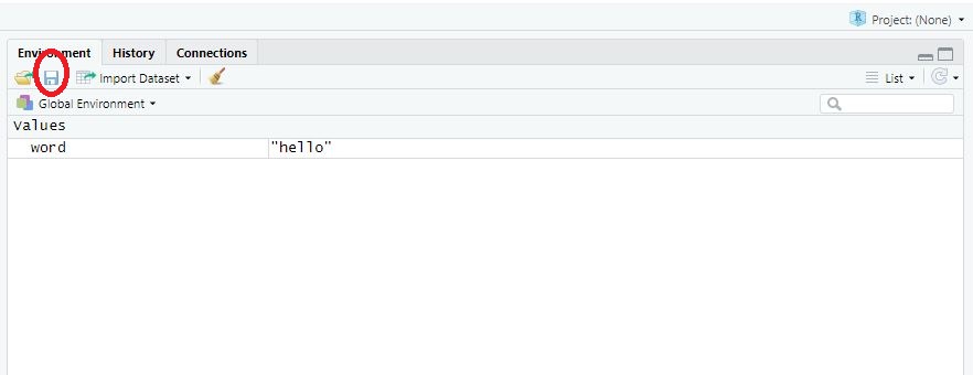
3.4.2 Save your results
You have successfully executed all commands and now want R to save your results/working environment? Saving your results is especially useful if it takes some time to have R run through the code and reproduce results - in this case, you only need to save results once and can then load them for the next session.
Again, there are several options for saving your results:
- Use the
save.image()-command:
- Use the save-button in the environment window and save your results in the correct format, for instance as MyData.RDATA”.
Image: Saving results
3.5 Help?!
The one thing you can count on in this seminar is that many things will not work right away: You’ll forget commands or what to use them for, the name of packages you need, or be confronted with errors messages that you need to understand to fix a given problem. This happens to anyone: from beginners to those having worked with R for many years. In this case, you need: help().
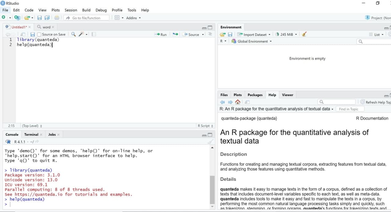
3.5.1 Find information about packages
If you’re interested in a specific package, you can also use R and the help() function(or simply use ?, which leads to the same result):
In turn, you’ll get more information via the window “Help”:
Image: Cran Overview for the Quanteda package
3.5.2 Find information about functions
Oftentimes, you need help with a specific function.
I’ll give you an example: Let’s say I teach a seminar with 10 students. I have asked all of them about their age. I have now saved their answers (i.e., 10 different numbers) in an object called age. This object is a vector, i.e. an object that consists of several values of the same data type - we’ll get to this in Tutorial 4.
Now we want R to compute the mean age of students in the seminar using the mean() function. We thus ask R to compute the mean of the vector age like so: We call the function mean(). We specify all necessary conditions to run it - here that x = age, i.e. that R should compute the mean of all values in the vector age:
## [1] 23.8That looks good - R tells us that the mean age of our students is 23.8 years. Let’s say I did the same thing for a different seminar: I also asked students about their age. while most chose to answer, some refused to answer. Thus, I recorded missing answers as NA (NA is used to record missing values, short for “not available”).
## [1] NAHowever, when trying to get the students’ mean age, R tells us that the mean is NA (i.e., missing). But do we really only have missing values? Let’s inspect our data again:
## [1] 23 26 NA 28 24 22 21 NA 24 NAThat’s not true: 7 out of 10 students told us their age; only 3 refused to answer (here recorded as NA). So why does R tell us that the overall mean is missing - shouldn’t the function simply ignore NAs and tells us the mean age of all of those 7 students who answered our question?
To do some troubleshooting, we use the help() function. We specify for which function we need help:
This is where our fourth window comes into place as results for our search for help are depicted here (the paragraph depicted here is the reference manual including information on the mean() function).
Image: Help for error with mean()-function
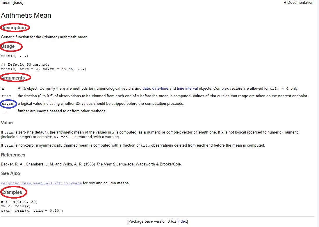
It includes important information on the function (of which we’ll discuss only some, namely those circled in red):
- Description: explains for which types of tasks the function
mean()should be used - Usage: explains how the function
mean()should be used - Arguments: explains which elements need to be or can be defined for using
mean()and how these elements need to be specified - Examples: exemplifies how the function
mean()can be used
When inspecting the section “Arguments”, we’ll soon discover something very important: mean() is a function that needs an object x for which the mean should be calculated. In this case, we specified x to consist of the vector x by typing x = age.
Upon further inspection, however, we see something else: The mean() function needs more information. In particular, we have to specify how R should deal with missing values, here NAs (see the section circled in red). This wasn’t a problem in the first example (since we had no NAs), but seems to be a problem for the second example. The manual reads as follows:
na.rm: a logical value indicating whether NA values should be stripped before the computation proceeds.
This indicates that if our x contains any NAs, we need to tell R and the mean() function how to deal with these. We haven’t specified this yet, which is why R includes all missing values for calculation and thus tells us that - given that some values are missing - the mean is missing. If we want R to ignore all NAs, we need to actively set na.rm (short for removal of NAs) to TRUE. This tells R that the mean should be computed for all of those values for x that are not missing.
The following command therefore gives us the mean age of all those students who chose to answer the question:
## [1] 243.5.3 Search for help online
For some questions, using the help() function won’t cut it. In this case, Google is your new best friend.
I have almost never encountered I problem I had with R where someone else had not already had the same problem and asked for answers online (and most often, had already gotten a helpful response.).
When googling, look out for the following websites that often offer help for statistical/programming issues:
3.5.3.1 Make sure to use relevant search terms
When googling, make sure to use all relevant search terms. This includes at least:
- parts of the error message you are receiving or descriptions of the error
- the search term “R” (there are a lot of other programming languages and you should make sure that your answers are tailored to R)
- the function throwing the error
Let’s say you are trying to find out how to set your working directory since your R throws the following error: “cannot find directory”. Googling for help via search terms such as “directory programming define” will likely lead to insufficient results because: (a) the specific command you are having trouble with is missing, (b) the specific error message you are getting is missing, (c) the search request does not specify that you need answers for the programming language R.
A better way to go around this would be something like: “setwd() R error message cannot find directory”: (a) you are specifying the command that gives you trouble, (b) you are specifying the error message, and (c) you are specifying that you want answers for R.
3.5.3.2 Don’t trust every result you get
While most Google searches will get you a multitude of different answers for your questions, not all of them are necessarily right for your specific problem. Moreover, there may be different solutions for the same problem - so don’t be confused when people are proposing different approaches. Contrary to common conception, the internet is not always right - you may also get answers that are wrong or inefficient. Its often best to scroll through some search results and then try the solution that seems most understandable and/or suitable for you.
3.5.3.3 Make your problem reproducible
It is often vital that others can reproduce your problem: Others need to see which lines of codes exactly created an error message, what the error message looked liked, which data you used, and on which type of machine/system you ran the analysis to help.
For instance: Nobody is likely going to be able to help you with a request like this:
"If I try to set my working directory, my computer tells me that I can't (the error says: Error: unpexted input in setwd(C:\. What is the problem?"This isn’t great because no one knows the code that created the problem or the machine/system you used. Thus, you need to make your error replicable by giving the exact command and potentially information about your machine via sessionInfo():
"I am trying to set my working directory on a Windows System using the following code:
setwd(C:\Users\vhase\Documents\Information-Flow)

While the path to the folder that I want to be my working directory is definitely correct, R gives me the following error message:
Error: unpexted input in setwd(C:\."## R version 4.3.1 (2023-06-16 ucrt)
## Platform: x86_64-w64-mingw32/x64 (64-bit)
## Running under: Windows 10 x64 (build 19045)
##
## Matrix products: default
##
##
## locale:
## [1] LC_COLLATE=English_United States.1252 LC_CTYPE=English_United States.1252 LC_MONETARY=English_United States.1252
## [4] LC_NUMERIC=C LC_TIME=English_United States.1252
## system code page: 65001
##
## time zone: Europe/Berlin
## tzcode source: internal
##
## attached base packages:
## [1] stats graphics grDevices utils datasets methods base
##
## other attached packages:
## [1] tokenizers_0.3.0 stringi_1.7.12 polite_0.1.3 rvest_1.0.3 dplyr_1.1.3 extrafont_0.19 bookdown_0.36
## [8] rsconnect_1.1.1
##
## loaded via a namespace (and not attached):
## [1] sass_0.4.7 utf8_1.2.3 generics_0.1.3 xml2_1.3.5 extrafontdb_1.0 digest_0.6.33 magrittr_2.0.3
## [8] evaluate_0.22 fastmap_1.1.1 jsonlite_1.8.7 robotstxt_0.7.13 httr_1.4.7 selectr_0.4-2 purrr_1.0.2
## [15] fansi_1.0.5 jquerylib_0.1.4 cli_3.6.1 rlang_1.1.1 withr_2.5.1 cachem_1.0.8 yaml_2.3.7
## [22] tools_4.3.1 memoise_2.0.1 ratelimitr_0.4.1 curl_5.1.0 assertthat_0.2.1 mime_0.12 vctrs_0.6.3
## [29] R6_2.5.1 lifecycle_1.0.3 stringr_1.5.0 fs_1.6.3 usethis_2.2.2 pkgconfig_2.0.3 pillar_1.9.0
## [36] bslib_0.5.1 Rcpp_1.0.11 glue_1.6.2 xfun_0.40 tibble_3.2.1 tidyselect_1.2.0 rstudioapi_0.15.0
## [43] knitr_1.44 spiderbar_0.2.5 SnowballC_0.7.1 htmltools_0.5.6.1 rmarkdown_2.25 Rttf2pt1_1.3.12 compiler_4.3.1
## [50] askpass_1.2.0 openssl_2.1.1💡 Take Aways
- Working Directory: The folder from which data can be imported into R or to which you can export and save data created with R. Should be defined at the beginning of each session. Commands:
setwd(),getwd() - Packages: Collections of topic-specific functions that extend the functions implemented in base R. You only need to install them once on your computer - but you have to activate packages at the beginning of each session. Otherwise, R will not be able to find related functions. Commands:
install.packages(),library() - Help: The thing everyone working with R needs. It’s normal to run into errors when working with R - don’t get frustrated too easily. Commands:
?,help() - Import data from working directory: Plenty of commands and packages for doing this - e.g.,
read.csv(). To load an existing workspace, useload() - Save code & results: You should save your code/results from time to time to be able to replicate analyses. Commands:
save.image
📚 More tutorials on this
You still have questions? The following tutorials & papers can help you with that:
📌 Test your knowledge
Task 3.1
Create a subfolder called “data” in your current working environment. Download the text file “data_halloween.txt” (via Moodle/Data for R). Save the text file in the subfolder and try to load it into R as an object called data_halloween.
Task 3.2
In this subfolder called “data”, try to write out the file you just created called data_halloween as a .csv file. You may have to google for the right command.
Task 3.3
If either of these tasks did not work: Try to formulate an online search request for how you would google for this error.
Let’s keep going: Tutorial 4: Objects & structures in R
A better option would be to use relative paths to your working directory. For simplicity, we will not be doing that in this seminar - but if you want to try it, see https://here.r-lib.org↩︎