4 Tutorial 4: Objects & structures in R
After working through Tutorial 4, you’ll…
- know about types of data in R (numbers, text, factors, dates, logical/other operators)
- know about types of objects in R (scalars, vectors, matrices, data frames, lists)
4.1 Types of data
Objects in R can contain a variety of different types of data. We’ll get to know a selection of these, namely
To understand and work with these types of data, we’ll now import a data set. Here, we’ll again use the Excel file “data_fictional_survey.csv” (via Moodle/Data for R).
Remember: The data set consists of data that is completely made up - a survey with 20 fictional students in a fictional seminar. We only use this data here so you can understand differences between types of data and types of objects.
##          name age       date outlet outlet_use outlet_trust
## 1   Alexandra  20 09.09.2021     TV          2            5
## 2        Alex  25 08.09.2021 Online          3            5
## 3  Maximilian  29 09.09.2021  Print          4            1
## 4      Moritz  22 06.09.2021     TV          2            2
## 5     Vanessa  25 07.09.2021 Online          1            3
## 6      Andrea  26 09.09.2021 Online          3            4
## 7    Fabienne  26 09.09.2021     TV          3            2
## 8       Fabio  27 09.09.2021 Online          0            1
## 9   Magdalena   8 08.09.2021 Online          1            4
## 10        Tim  26 07.09.2021     TV         NA            2
## 11       Alex  27 09.09.2021 Online         NA            2
## 12     Tobias  26 07.09.2021 Online          2            2
## 13    Michael  25 09.09.2021 Online          3            2
## 14    Sabrina  27 08.09.2021 Online          1            2
## 15   Valentin  29 09.09.2021     TV          1            5
## 16    Tristan  26 09.09.2021     TV          2            5
## 17     Martin  21 09.09.2021 Online          1            2
## 18       Anna  23 08.09.2021     TV          3            3
## 19    Andreas  24 09.09.2021     TV          2            5
## 20    Florian  26 09.09.2021 Online          1            5
4.1.1 Numbers
A typical type of data you may come is numeric data. In our data set, the age of respondents is saved as numbers.
In R, this type of data is called numeric. To check if age is really saved as numbers, you can use mode(). The function tells you an object’s type.
## [1] "numeric"4.1.2 Text
In this seminar, we will often work with letters, words, or whole texts. Such text is saved in the character format. In our data set, we know that the variable name is likely to contain textual content. We’ll check this with the same command mode():
## [1] "character"You may have already spotted something else: If you want to save something in character format, you have to set quotation marks ““ before and after the respective values. For instance, if you save the number 1 with quotation marks, R will use the character format:
## [1] "character"However, if you save the number 1 without quotation marks, R will use the numeric format:
## [1] "numeric"Why is this important? In R, many functions for conducting statistical analyses, for example, can only be executed with objects containing numeric data, not character data.
For instance: Let’s say you want R to calculate the mean of some numbers:
R will throw you an error message. Why? Because you saved these numbers as character values, not as numeric values:
## [1] "character"If we save these numbers in a numeric format, i.e., as numbers not text, the command works just fine:
## [1] 5.54.1.3 Factors
Factors constitute an additional type of data. Factors can include both numeric data and characters. What is important, however, is that they treat any types of data as categorical.
We can, for instance, convert the variable name - which now contains each student’s name in character format - to a factor using as.factor():
As you can see, the variable age now contains each name as an independent level. You can get each unique level with the levels() command:
##  [1] "Alex"       "Alexandra"  "Andrea"     "Andreas"    "Anna"       "Fabienne"   "Fabio"      "Florian"    "Magdalena"  "Martin"
## [11] "Maximilian" "Michael"    "Moritz"     "Sabrina"    "Tim"        "Tobias"     "Tristan"    "Valentin"   "Vanessa"
You may have noted that the data set survey contains 20 observations but that the variable age only included 19 levels. Why? If you inspect the data set, you can see that two students have the same name (here, Alex in row 2 and 11) - which is why we have 20 observations, but only 19 unique levels for the variable name:
##          name age       date outlet outlet_use outlet_trust
## 1   Alexandra  20 09.09.2021     TV          2            5
## 2        Alex  25 08.09.2021 Online          3            5
## 3  Maximilian  29 09.09.2021  Print          4            1
## 4      Moritz  22 06.09.2021     TV          2            2
## 5     Vanessa  25 07.09.2021 Online          1            3
## 6      Andrea  26 09.09.2021 Online          3            4
## 7    Fabienne  26 09.09.2021     TV          3            2
## 8       Fabio  27 09.09.2021 Online          0            1
## 9   Magdalena   8 08.09.2021 Online          1            4
## 10        Tim  26 07.09.2021     TV         NA            2
## 11       Alex  27 09.09.2021 Online         NA            2
## 12     Tobias  26 07.09.2021 Online          2            2
## 13    Michael  25 09.09.2021 Online          3            2
## 14    Sabrina  27 08.09.2021 Online          1            2
## 15   Valentin  29 09.09.2021     TV          1            5
## 16    Tristan  26 09.09.2021     TV          2            5
## 17     Martin  21 09.09.2021 Online          1            2
## 18       Anna  23 08.09.2021     TV          3            3
## 19    Andreas  24 09.09.2021     TV          2            5
## 20    Florian  26 09.09.2021 Online          1            5
4.1.4 Missing data/NAs
Something we will often encounter is missing data, also called NAs. In our data set, the variable outlet_use which describes how many hours a day a student uses a specific outlet contains missing data:
## [1] 2 3 4 2 1 3 3 0 1 NA NA 2 3 1 1 2 1 3 2 1When working with data, you should always check how much of it may be missing (and of course, why). To do so, you can use the is.na() command: It tells you which values in a specific objects are missing (TRUE) or not missing (FALSE):
## [1] FALSE FALSE FALSE FALSE FALSE FALSE FALSE FALSE FALSE TRUE TRUE FALSE FALSE FALSE FALSE FALSE FALSE FALSE FALSE FALSEFor instance, the first 9 observations do not contain any missing values for the variable age, but the 10th observation does.
With larger data sets, you obviously would not want to check this manually for every single observation. We can use a little trick here: Since the value FALSE counts as 0 and the value TRUE counts as a 1…
## [1] 0## [1] 1… we can simply calculate the sum of these values for survey$outlet_use to see whether how many observations are missing:
## [1] 24.1.5 Logical/other operators
Lastly, you should know about logical (or other) operators. These are often used to check whether certain statements are true/false, whether some values take on a certain value or not, or whether some values are higher/lower than others. Since we won’t need this right away,I won’t go into details here - but we will need these later:
| Operator | Meaning |
|---|---|
| TRUE | indicates that a certain statement applies, i.e., is true |
| FALSE | indicates that a certain statement does not apply, i.e., is not true |
| & | connects two statements which should both be true |
| | | connects two statements of which at least one should be true |
| == | indicates that a certain value should equal another one |
| != | indicates that a certain value should not equal another one |
| > | indicates that a certain value should be larger than another one |
| < | indicates that a certain value should be smaller than another one |
| >= | indicates that a certain value should be larger than or equal to another one |
| <= | indicates that a certain value should be smaller than or equal to another one |
You may wonder: Why should I use this?
Glad you asked: We’ll need these operators, for instance, to filter data sets by specific values or apply functions if some conditions (but not others) are true.
For instance, you could use a logical operator to only keep those students in the data set that are older than 21 (17 out of 20 students). We filter the data set using the > operator. We can get basic information about this data set using the str() command:
## 'data.frame':    17 obs. of  6 variables:
##  $ name        : Factor w/ 19 levels "Alex","Alexandra",..: 1 11 13 19 3 6 7 15 1 16 ...
##  $ age         : int  25 29 22 25 26 26 27 26 27 26 ...
##  $ date        : chr  "08.09.2021" "09.09.2021" "06.09.2021" "07.09.2021" ...
##  $ outlet      : chr  "Online" "Print" "TV" "Online" ...
##  $ outlet_use  : int  3 4 2 1 3 3 0 NA NA 2 ...
##  $ outlet_trust: int  5 1 2 3 4 2 1 2 2 2 ...
4.2 Types of objects
Great, now you know all about types of data. As promised, this tutorial will also teach you about different types of objects:
4.2.1 Scalars
The “smallest” type of data you will encounter are scalars.
Scalars are objects consisting of a single value - for example, a letter, a word, a sentence, a number, etc.
You’ve already seen what a scalar looks like - remember the very first time you were [Writing Code]? Here, we defined an objects word which only consisted of the word “hello”.
## [1] "hello"We could also save a single number this way:
## [1] 1The same applies to a single sentence:
## [1] "I would like to be saved as a scalar"4.2.2 Vectors
The next type of data you should know are vectors:
Vectors are objects that consist of several values of the same type of data.
For instance, if we want to save several words or numbers separately, we can save them as vectors. This means that the first element of our vector will be our first word, the second the second word and so forth. Importantly, a vector can only contain data of the same type - for instance, you cannot save data in numeric and character format in the same format.
In principle, you can often (but not always) compare vectors with variables in data sets: They contain values for all observations in your data set (with all of these values being of the same data type).
An example would be the numbers from 1 to 20 that we worked with before. Now, it becomes apparent what the c() stands for - it specifies the vector format.
We define the object numbers to consist of the a vector c() which contains the values 1 to 20. Here, we ask R to include all values from 1 to 20 by inserting a colon between both numbers:
## [1] 1 2 3 4 5 6 7 8 9 10 11 12 13 14 15 16 17 18 19 20If you want the vector numbers to only contain selected numbers from 1 to 20, you can specify these numbers and separate them using a comma:
## [1] 1 5 8 19 20We can do the same thing for data in character format:
## [1] "Apple" "Banana" "Orange" "Lemon"In practice, a vector is nothing else than scalars of the same typed chained together - in this case, the words “Apple”, “Banana”, “Orange”, and “Lemon”.
If you love to write inefficient code, you could also define separate objects (here: scalars) consisting of every element of the vector you want to define and then chain them together (10/10 wouldn’t recommend because this is unnecessarily complicated):
apple <- "Apple"
banana <- "Banana"
orange <- "Orange"
lemon <- "Lemon"
fruits <- c(apple, banana, orange, lemon)
fruits
## [1] "Apple" "Banana" "Orange" "Lemon"This would lead to very similar results, but you would have to write 4 more lines of code compared to the previous example.
4.2.3 Data frames & matrices
An even “bigger” type of data, in this sense, are data frames and matrices:
Data frames & matrices consist of several vectors of the same length.
Matrices and data frames come closest to how you may understand data sets (for instance, in SPSS). Our survey data set is one example for a data frame:
##          name age       date outlet outlet_use outlet_trust
## 1   Alexandra  20 09.09.2021     TV          2            5
## 2        Alex  25 08.09.2021 Online          3            5
## 3  Maximilian  29 09.09.2021  Print          4            1
## 4      Moritz  22 06.09.2021     TV          2            2
## 5     Vanessa  25 07.09.2021 Online          1            3
## 6      Andrea  26 09.09.2021 Online          3            4
## 7    Fabienne  26 09.09.2021     TV          3            2
## 8       Fabio  27 09.09.2021 Online          0            1
## 9   Magdalena   8 08.09.2021 Online          1            4
## 10        Tim  26 07.09.2021     TV         NA            2
## 11       Alex  27 09.09.2021 Online         NA            2
## 12     Tobias  26 07.09.2021 Online          2            2
## 13    Michael  25 09.09.2021 Online          3            2
## 14    Sabrina  27 08.09.2021 Online          1            2
## 15   Valentin  29 09.09.2021     TV          1            5
## 16    Tristan  26 09.09.2021     TV          2            5
## 17     Martin  21 09.09.2021 Online          1            2
## 18       Anna  23 08.09.2021     TV          3            3
## 19    Andreas  24 09.09.2021     TV          2            5
## 20    Florian  26 09.09.2021 Online          1            5
Let’s say we don’t have a data set yet but want to create one ourselves. For instance, we have three vectors of the same length that contain the following data:
- a vector called fruits consisting of the names of four different fruits (character)
- a vector called price consisting of the amount of money each fruit costs (numeric)
- a vector called color consisting of the color of each fruit (character)
fruits <- c("Apple", "Banana", "Orange", "Lemon")
price <- c(0.8,0.6,0.78,0.9)
color <- c("red", "yellow", "orange", "yellow")
Since these vectors describe the same data, we want them to be saved as one data set. To create the data set data_fruits, we use the command data.frame(), which contains:
- an vector called fruits as its first column
- a vector called price as its second column
- a vector color as its third column
Here, columns describe different variables and rows observations.
##   fruits price  color
## 1  Apple  0.80    red
## 2 Banana  0.60 yellow
## 3 Orange  0.78 orange
## 4  Lemon  0.90 yellow
In difference to data frames that can encompass different types of data, matrices consist of vectors of exactly the same type of data - for instance, only character vectors or numeric vectors.
This is also why we will mostly be working with data frames in this seminar - they are just more flexible and more suitable for the data we will work with. The data frame “version” in tidyverse is called tibbles.
For a nice example for comparing scalars, vectors, data frames, and matrices, check out this example here.
4.2.4 Lists
Lastly, you should know about lists.
Lists can be described as an array of (different) objects.
As discussed before, data frames can encompass vectors consisting of different types of data (for instance, character and numeric vectors). However, these all have to be vectors (and of the same length). In some case, you may want to save very different types of objects - scalars, vectors, data frames, and objects -, which will differ in length3.
In this case, lists offer the most flexible way of saving very different objects within one object (i.e., the list). Let’s say that we want to save our data frame data_fruits as well the data frame survey in a single object. We do so by specifying a list which includes data_fruits as its first and survey as its second element:
Image: List
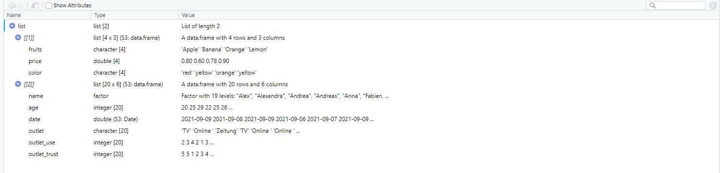
As you see, the object list consists of two elements:
- the first element [[1]] encompasses the data frame data_fruits
- the second element [[2]] encompasses the data frame survey
4.2.5 Other types of objects
Since we’ll be learning how to conduct automated content analysis in this tutorial, we’ll encounter a bunch of other types of data such as the corpus or the document-feature-matrix (dfm). You don’t have to know anything about these data types for now - just be aware that other types of objects exist.
💡 Take Aways
- Types of data: In R, you can work with different types of data in numeric, character, factor, or data format. Important commands: mode(), str(), as.character(), as.numeric(), as.factor(), levels(), & is.na()
- Types of objects: In R, you can work with different types of objects, for instance scalars, vectors, data frames, matrices, or lists. Important commands: c(), data.frame(), list()
📚 More tutorials on this
You still have questions? The following tutorials & papers can help you with that:
📌 Test your knowledge
You’ve worked through all the material of Tutorial 4? Let’s see it - the following tasks will test your knowledge.
Task 4.1
Create a data frame called data. The data frame should contain the following variables (in this order):
- a vector called food. It should contain 5 elements, namely the names of your five favourite dishes.
- a vector called description. For every dish mentioned in food, please describe the dish in a single sentence (for instance, if the first food you describe is “pizza”, you could write: “This is an Italian dish, which I prefer with a lot of cheese.”)
- a vector called rating. Rate every dish mentioned in food with 1-5 (using every number only once), i.e., by rating your absolute favorite dish out of all five with a 1 and your least favorite dish out of all five with a 5.
Hint: For me, the data frame would look something like this:
##            food                                             description Rating
## 1         pizza Italian dish, I actually prefer mine with little cheese      3
## 2         pasta                                    Another Italian dish      1
## 3     ice cream                             The perfect snack in summer      2
## 4        crisps              Potatoes and oil - a luxurious combination      4
## 5 passion fruit             A fruit that makes me think about  vacation      5
Task 4.2
Can you sort the data in your data set by rating - with your favorite dish (i.e., the one rated “1”) on top of the list and your least favorite dish (i.e., the one rated “5”) on the bottom?
Important: You do not yet know this command - you’ll have to google for the right solution. Please do and note down the exact search terms you used for searches via Google, so we can discuss them next week.
Hint: For me, the data frame would look something like this:
##            food                                             description Rating
## 1         pasta                                    Another Italian dish      1
## 2     ice cream                             The perfect snack in summer      2
## 3         pizza Italian dish, I actually prefer mine with little cheese      3
## 4        crisps              Potatoes and oil - a luxurious combination      4
## 5 passion fruit             A fruit that makes me think about  vacation      5
This is where you’ll find solutions for Tutorial 4.
Let’s keep going: Tutorial 5: Data management with tidyverse.
Length means that these objects may contain different numbers of elements (in the case of scalars and vectors, for example) or different numbers of rows/columns (in the case of data frames and matrices, for example)↩︎