FreeSurfer

recon-all

There are three main components to FreeSurfer’s output: quality control measure, cortical parcellation, subcortical segmentation. If available, longitudinal analyses of all the regions can also be provided.

FreeSurfer’s Euler number summarizes the topological complexity of the reconstructed cortical surface. The Euler number can be used to identify images as unusable and is a highly reliable measure of image quality.
From FreeSurfer’s cortical parcellation several measures can be obtained from within each region: surface area, cortical thickness, gray matter volume, white matter volume, and cortical mean curvature.
From FreeSurfer’s subcortical segmentation, volumes can be obtained.
Percentage change and raw values can also be obtained through longitudinal pipelines.

Basic command:

recon-all \
-subjid ${SUBJ}_${SES} \
-i ${DERIV}/${SUBJ}_${SES}_T1w.nii.gz \
-wsatlas \ # Use atlas instead of watershed threshold
-all \
-sd ${DERIV}/freesurfer

Include T2 or FLAIR:

recon-all \
-subjid ${SUBJ}_${SES} \
-i ${DERIV}/${SUBJ}_${SES}_T1w.nii.gz \
-T2 ${DERIV}/${SUBJ}_${SES}_inplaneT2w.nii.gz \
-T2pial \
-wsatlas \
-all \
-sd ${DERIV}/freesurfer

recon-all \
-subjid ${SUBJ}_${SES} \
-i ${DERIV}/${SUBJ}_${SES}_T1w.nii.gz \
-FLAIR ${DERIV}/${SUBJ}_${SES}_inplaneFLAIR.nii.gz \
-FLAIRpial \
-wsatlas \
-all \
-sd ${DERIV}/freesurfer

Analyze just one hemisphere:

recon-all \
-subjid ${SUBJ}_${SES} \
-i ${DERIV}/${SUBJ}_${SES}_T1w.nii.gz \
-T2 ${DERIV}/${SUBJ}_${SES}_inplaneT2w.nii.gz \
-T2pial \
-wsatlas \
-all \
-hemi lh \ # lh or rh
-sd ${DERIV}/freesurfer

If your study includes participants with larger than normal ventricles (e.g., cancer, Alzheimer’s):

recon-all \
-subjid ${SUBJ}_${SES} \
-i ${DERIV}/${SUBJ}_${SES}_T1w.nii.gz \
-T2 ${DERIV}/${SUBJ}_${SES}_inplaneT2w.nii.gz \
-T2pial \
-wsatlas \
-all \
-bigventricles
-sd ${DERIV}/freesurfer

Euler

After Leonhard Euler (1707-83), the Euler number is a topological invariant of a surface that can be computed from the number of edges, vertices and faces in a polygonal tessellation. For a completely flat and smooth surface with no handles or holes, the Euler value should be 2. For a surface that contains a lot of holes or handles, the Euler number is 2-2n, where n is the number of defects. The higher the Euler number, the higher the data quality for FreeSurfer cortical reconstruction. In other words, the less negative the number the better. Unfortunately, there’s no set number for determining quality as the number varies between populations (i.e., adolescents vs. adults), and across scanners and sequences. The Euler value can only be used within a study to determine quality control issues (Rosen et al., 2018). However, it has been proposed that the Euler value may be used towards optimization and standardization of scans across sites (Chalavi, Simmons, Dijkstra, Barker, & Reinders, 2012).

Subcortical Segmentation (aseg)

Load white matter and pial segmentation plus aseg file:

freeview -v \
mri/T1.mgz \
mri/wm.mgz \
mri/brainmask.mgz \
mri/aseg.mgz:colormap=lut:opacity=0.2 \
-f surf/lh.white:edgecolor=yellow \
surf/lh.pial:edgecolor=red \
surf/rh.white:edgecolor=yellow \
surf/rh.pial:edgecolor=red \
--viewport coronal \
--layout 1 \
--viewsize 800 800 \
--zoom 1.5

Volume in mm³

The hippocampus and amygdala volumes in this file are WRONG. Please verify the ROIs of any other subcortical region before using as these segmentations are often inaccurate. Refer to the seperate hippocampus / amygdala, brainstem, and thalamus pipelines.

asegstats2table \
--subjectsfile subjects.txt \
--meas volume \
--skip \
--delimiter comma \
--tablefile tablefiles/aseg-volume-stats.csv

Cerebral White Matter
Lateral Ventricle
Inferior Lateral Ventricle
Cerebellum White Matter
Cerebellum Cortex
Caudate
Putamen
Pallidum
Lesions
Accumbens area
Vessel
Third Ventricle
Fourth Ventricle
Cerebrospinal Fluid
Corpus Callosum (Posterior, Mid Posterior, Central, Mid Anterior, Anterior)
…and more

DO NOT USE HIPPOCAMPUS, AMYGDALA, THALAMUS, AND BRAINSTEM VOLUMES FROM THE ASEG FILE!

Cortical Parcellation (aparc)

View pial, white matter, inflated white matter, thickness, and parcellation in 3D:

freeview -f  surf/lh.pial:annot=aparc.annot:name=pial_aparc:visible=0 \
surf/lh.inflated:overlay=lh.thickness:overlay_threshold=0.1,3::name=inflated_thickness:visible=0 \
surf/lh.inflated:visible=0 \
surf/lh.white:visible=0 \
surf/lh.pial \
--viewport 3d

Area in mm²

for i in lh rh; do
  aparcstats2table \
  --subjectsfile subjects.txt \
  --hemi $i \
  --meas area \
  --skip \
  --delimiter comma \
  --tablefile tablefiles/aparc-area-${i}-stats.csv
done

Volume in mm³

for i in lh rh; do
  /Applications/freesurfer-dev/bin/aparcstats2table \
  --subjectsfile subjects.txt \
  --hemi $i \
  --meas volume \
  --skip \
  --delimiter comma \
  --tablefile tablefiles/aparc-volume-${i}-stats.csv
done

White Matter Volume in mm³

asegstats2table \
--stats wmparc.stats \
--subjectsfile subjects.txt \
--meas volume \
--skip \
--delimiter comma \
--tablefile tablefiles/wmparc-volume-stats.csv

Cortical Thickness in mm

for i in lh rh; do
  aparcstats2table \
  --subjectsfile subjects.txt \
  --hemi $i \
  --meas thickness \
  --skip \
  --delimiter comma \
  --tablefile tablefiles/aparc-thickness-${i}-stats.csv
done

Mean Curvature

for i in lh rh; do
  aparcstats2table \
  --subjectsfile subjects.txt \
  --hemi $i \
  --meas meancurv \
  --skip \
  --delimiter comma \
  --tablefile tablefiles/aparc-meancurv-${i}-stats.csv
done

Compare Atlases

freeview -v \
mri/orig.mgz \
mri/aparc+aseg.mgz:colormap=lut:opacity=0.4 \
mri/aparc.a2009s+aseg.mgz:colormap=lut:opacity=0.4

APARC Parcellations by Lobes

Frontal

Superior Frontal
Rostral and Caudal Middle Frontal
Pars Opercularis, Pars Triangularis, and Pars Orbitalis
Lateral and Medial Orbitofrontal
Precentral
Paracentral
Frontal Pole

Parietal

Superior Parietal
Inferior Parietal
Supramarginal
Postcentral
Precuneus

Temporal

Superior, Middle, and Inferior Temporal
Banks of the Superior Temporal Sulcus
Fusiform
Transverse Temporal
Entorhinal
Temporal Pole
Parahippocampal

Occipital

Lateral Occipital
Lingual
Cuneus
Pericalcarine

Cingulate (if you want to include in a lobe)

Rostral Anterior (Frontal)
Caudal Anterior (Frontal)
Posterior (Parietal)
Isthmus (Parietal)

Other

Insula

Hippocampus & Amygdala

After running recon-all:

segmentHA_T1.sh \
${SUBJ}_${SES} \
${DERIV}/freesurfer/

To visualize the segmentations:

freeview -v \
mri/T1.mgz \
-v mri/lh.hippoAmygLabels-T1.v21.CA.mgz:colormap=lut:opacity=0.3 \
-v mri/rh.hippoAmygLabels-T1.v21.CA.mgz:colormap=lut:opacity=0.3 \
--viewport coronal \
--layout 1 \
--viewsize 800 800 \
--zoom 1.5

Output results to CSV:

quantifyHAsubregions.sh hippoSf T1 tablefiles/hipposubfields-stats.csv
quantifyHAsubregions.sh amygNuc T1 tablefiles/amygdalarnuclei-stats.csv
sed -i '' 's/ /,/g' tablefiles/hipposubfields-stats.csv
sed -i '' 's/ /,/g' tablefiles/amygdalarnuclei-stats.csv

You can also include T2 with these analyses:

segmentHA_T2.sh \
${SUBJ}_${SES} \
${DERIV}/${SUBJ}_${SES}_inplaneT2w.nii.gz \
T2 \
1 \
${DERIV}/freesurfer/

To extract those values:

quantifyHAsubregions.sh hippoSf T1-T2 tablefiles/hipposubfields-stats.csv
quantifyHAsubregions.sh amygNuc T1-T2 tablefiles/amygdalarnuclei-stats.csv
sed -i '' 's/ /,/g' tablefiles/hipposubfields-stats.csv
sed -i '' 's/ /,/g' tablefiles/amygdalarnuclei-stats.csv

Hippocampus

If you have used results from this software for a publication, please use this citation (Iglesias, Augustinack, et al., 2015).

Hippocampal Tail
Hippocampal Body
Hippocampal Head
Whole Hippocampus
Subiculum
Presubiculum
Parasubiclum
CA1
CA3
CA4
Molecular layer
Fimbria
Hippocampal fissure
HATA

Amygdala

In addition, if you have used the segmentation of the nuclei of the amygdala, please also cite (Saygin et al., 2017).

Whole amygdala
Lateral nucleus
Basal nucleus
Accessory basal nucleus
Anterior amygdaloid area
Central nucleus
Medial nucleus
Cortical nucleus
Corticoamygdaloid transition area
Paralaminar nucleus

Brainstem

After running recon-all:

segmentBS.sh \
${SUBJ}_${SES} \
${DERIV}/freesurfer/

To view the segmentation:

freeview -v \
mri/nu.mgz \
-v mri/brainstemSsLabels.v12.mgz:colormap=lut:opacity=0.3 \
--viewport coronal \
--layout 1 \
--viewsize 800 800 \
--zoom 1.5

Output results to CSV:

quantifyBrainstemStructures.sh tablefiles/brainstem-stats.csv
sed -i '' 's/ /,/g' tablefiles/brainstem-stats.csv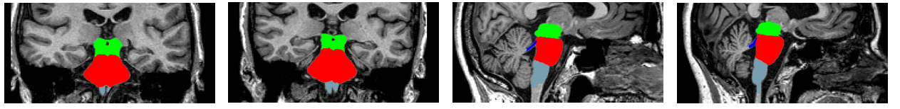

If you have used results from this software for a publication, please use this citation (Iglesias, Van Leemput, et al., 2015).

Whole brainstem
Medulla
Pons
Midbrain
Superior cerebellar peduncles

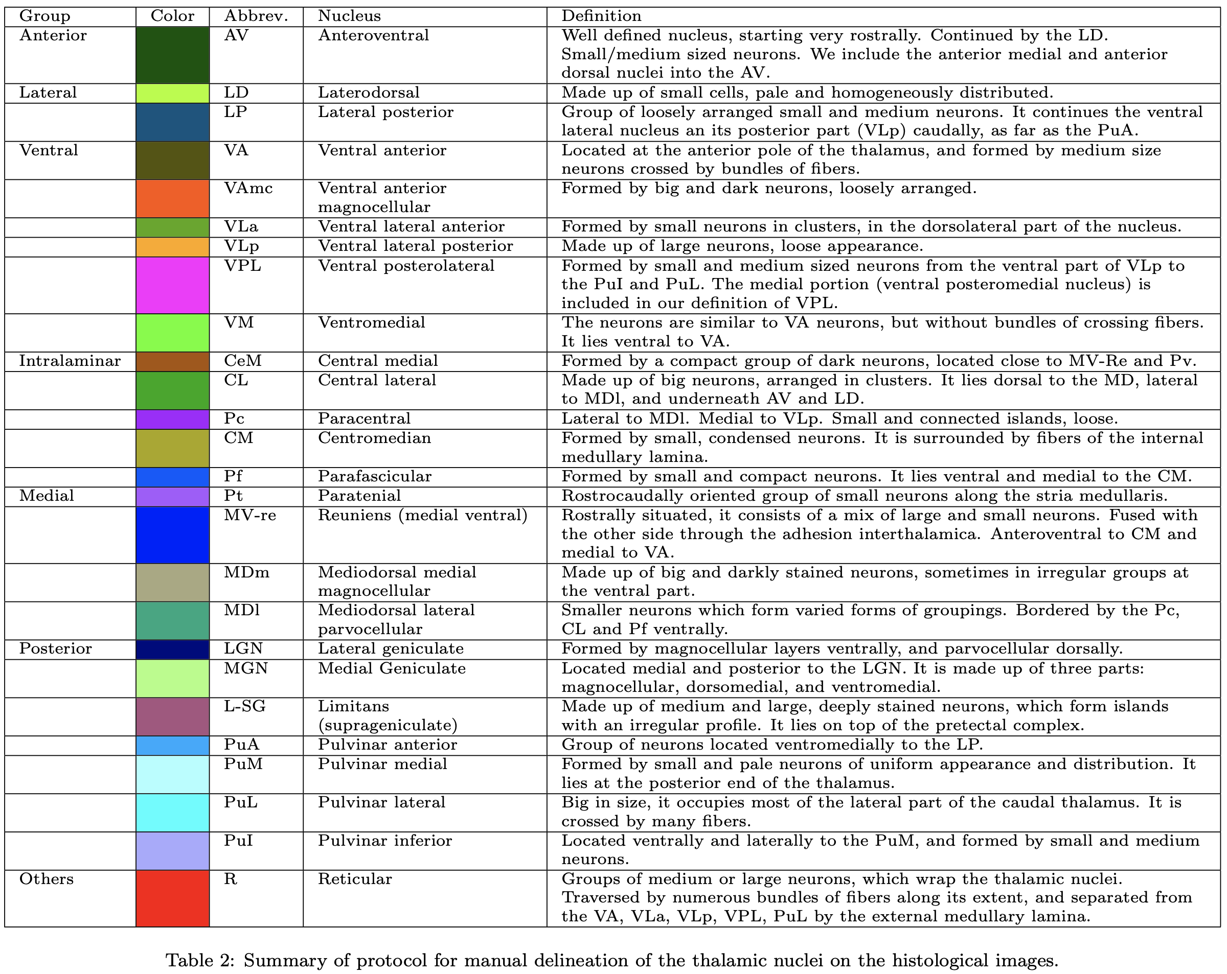
Thalamus

After running recon-all:

segmentThalamicNuclei.sh \
${SUBJ}_${SES} \
${DERIV}/freesurfer/

Output results to CSV:

quantifyThalamicNuclei.sh tablefiles/thalamicnuclei-stats.csv T1
sed -i '' 's/ /,/g' tablefiles/thalamicnuclei-stats.csv

If you have used results from this software for a publication, please use this citation (Iglesias et al., 2018).

Longitudinal Analyses

Unbiased Subject Template

recon-all \
-base ${SUBJ} \
-tp ${SUBJ}_ses-1 \
-tp ${SUBJ}_ses-2 \
-all \
-sd ${DERIV}/freesurfer/

Longitudinal Analysis

Process session 1:

recon-all \
-long \
${SUBJ}_ses-1 \
${SUBJ} \
-all \
-sd ${DERIV}/freesurfer/

Process session 2:

recon-all \
-long \
${SUBJ}_ses-2 \
${SUBJ} \
-all \
-sd ${DERIV}/freesurfer/

As quoted from the FreeSurfer website:

Cortical reconstruction and volumetric segmentation was performed with the Freesurfer image analysis suite, which is documented and freely available for download online (http://surfer.nmr.mgh.harvard.edu/). The technical details of these procedures are described in prior publications (Dale, Fischl, & Sereno, 1999; Bruce Fischl & Dale, 2000; Bruce Fischl, Kouwe, et al., 2004; B. Fischl, Liu, & Dale, 2001; B. Fischl et al., 2002; Bruce Fischl, Salat, et al., 2004; Bruce Fischl, Sereno, & Dale, 1999; Bruce Fischl, Sereno, Tootell, & Dale, 1999; Han et al., 2006; Jovicich et al., 2006; Reuter & Fischl, 2011; Reuter, Schmansky, Rosas, & Fischl, 2012; Segonne et al., 2004). Briefly, this processing includes motion correction and averaging (Reuter, Rosas, & Fischl, 2010) of multiple volumetric T1 weighted images (when more than one is available), removal of non-brain tissue using a hybrid watershed/surface deformation procedure (Segonne et al., 2004), automated Talairach transformation, segmentation of the subcortical white matter and deep gray matter volumetric structures (including hippocampus, amygdala, caudate, putamen, ventricles) (B. Fischl et al., 2002; Bruce Fischl, Salat, et al., 2004) intensity normalization (Sled, Zijdenbos, & Evans, 1998), tessellation of the gray matter white matter boundary, automated topology correction (B. Fischl, Liu, & Dale, 2001; Segonne, Pacheco, & Fischl, 2007), and surface deformation following intensity gradients to optimally place the gray/white and gray/cerebrospinal fluid borders at the location where the greatest shift in intensity defines the transition to the other tissue class (Dale, Fischl, & Sereno, 1999; Bruce Fischl & Dale, 2000). Once the cortical models are complete, a number of deformable procedures can be performed for further data processing and analysis including surface inflation (Bruce Fischl, Sereno, & Dale, 1999), registration to a spherical atlas which is based on individual cortical folding patterns to match cortical geometry across subjects (Bruce Fischl, Sereno, Tootell, & Dale, 1999), parcellation of the cerebral cortex into units with respect to gyral and sulcal structure (Desikan et al., 2006; Bruce Fischl, Kouwe, et al., 2004), and creation of a variety of surface based data including maps of curvature and sulcal depth. This method uses both intensity and continuity information from the entire three dimensional MR volume in segmentation and deformation procedures to produce representations of cortical thickness, calculated as the closest distance from the gray/white boundary to the gray/CSF boundary at each vertex on the tessellated surface (Bruce Fischl & Dale, 2000). The maps are created using spatial intensity gradients across tissue classes and are therefore not simply reliant on absolute signal intensity. The maps produced are not restricted to the voxel resolution of the original data thus are capable of detecting submillimeter differences between groups. Procedures for the measurement of cortical thickness have been validated against histological analysis (Rosas et al., 2002) and manual measurements (Kuperberg et al., 2003; Salat et al., 2004). Freesurfer morphometric procedures have been demonstrated to show good test-retest reliability across scanner manufacturers and across field strengths (Han et al., 2006; Reuter, Schmansky, Rosas, & Fischl, 2012).

To extract reliable volume and thickness estimates, images are automatically processed with the longitudinal stream (Reuter, Schmansky, Rosas, & Fischl, 2012) in FreeSurfer. Specifically an unbiased within-subject template space image is created using robust, inverse consistent registration (Reuter, Rosas, & Fischl, 2010). Several processing steps, such as skull stripping, Talairach transforms, atlas registration as well as spherical surface maps and parcellations are then initialized with common information from the within-subject template, significantly increasing reliability and statistical power (Reuter, Schmansky, Rosas, & Fischl, 2012).

Please cite at least (Reuter, Schmansky, Rosas, & Fischl, 2012) if the longitudinal stream was used!

Hippocampus & Amygdala Longitudinal

After running longitudinal recon-all:

segmentHA_T1_long.sh \
${SUBJ}_${SES}_long.${SUBJ} \
${DERIV}/freesurfer/

Output results to CSV files:

quantifyHAsubregions.sh \
hippoSf \
T1.long \
${DERIV}/freesurfer/tablefiles/hipposubfields-long-stats.csv \
${DERIV}/freesurfer/

quantifyHAsubregions.sh \
amygNuc \
T1.long \
${DERIV}/freesurfer/tablefiles/amygdalarnuclei-long-stats.csv \
${DERIV}/freesurfer/

Files

FreeSurfer Subjects Directory

All freesurfer directories are located under the derivatives directory located in each BIDS organized dataset:

STUDY_DIR/
|–– derivatives/
    |–– pT1T2/
    |–– freesurfer/
|–– sub-001/
|–– sub-002/
|–– sub-003/
participants.tsv
dataset_description.json

If the dataset does not contain multiple sessions, the freesurfer directory will be organized in the following manner:

./freesurfer_subjects
$ Analysis of sub-001
├── sub-001
│   ├── label
│   ├── mri
│   ├── scripts
│   ├── stats
│   ├── surf
│   ├── tmp
│   ├── touch
│   └── trash
$ Analysis of sub-002
└── sub-002
    ├── label
    ├── mri
    ├── scripts
    ├── stats
    ├── surf
    ├── tmp
    ├── touch
    └── trash

However if you have multiple timepoints and the longitudinal stream was run, then you’ll have multiple directories for each participant. First, each timepoint is processed independently, which outputs cross-sectional results. In the FreeSurfer directory the time points will be named:

./freesurfer_subjects
$ Cross sectional analysis of sub-001 at timepoint 1
├── sub-001_ses-1
│   ├── label
│   ├── mri
│   ├── scripts
│   ├── stats
│   ├── surf
│   ├── tmp
│   ├── touch
│   └── trash
$ Cross sectional analysis of sub-001 at timepoint 2
└── sub-001_ses-2
    ├── label
    ├── mri
    ├── scripts
    ├── stats
    ├── surf
    ├── tmp
    ├── touch
    └── trash

Next, a within subject template is created across all time points. This is called the base directory and will just consist of the subject ID and not contain any session information. There should be only one base directory per subject. The data contained in this directory is not to be used for any analyses!

./freesurfer_subjects
$ Base template for sub-001 across all timepoints
├── sub-001
│   ├── label
│   ├── mri
│   ├── scripts
│   ├── stats
│   ├── surf
│   ├── tmp
│   ├── touch
│   └── trash
$ Cross sectional analysis of sub-001 at timepoint 1
├── sub-001_ses-1
│   ├── label
│   ├── mri
│   ├── scripts
│   ├── stats
│   ├── surf
│   ├── tmp
│   ├── touch
│   └── trash
$ Cross sectional analysis of sub-001 at timepoint 2
└── sub-001_ses-2
   ├── label
   ├── mri
   ├── scripts
   ├── stats
   ├── surf
   ├── tmp
   ├── touch
   └── trash

Finally, there will be longitudinal directories for each session.They contain the final, most reliable and accurate processing results that can be used.

./freesurfer_subjects
$ Base template for sub-001 across all timepoints
├── sub-001
│   ├── label
│   ├── mri
│   ├── scripts
│   ├── stats
│   ├── surf
│   ├── tmp
│   ├── touch
│   └── trash
$ Cross sectional analysis of sub-001 at timepoint 1
├── sub-001_ses-1
│   ├── label
│   ├── mri
│   ├── scripts
│   ├── stats
│   ├── surf
│   ├── tmp
│   ├── touch
│   └── trash
$ Cross sectional analysis of sub-001 at timepoint 2
├── sub-001_ses-2
│   ├── label
│   ├── mri
│   ├── scripts
│   ├── stats
│   ├── surf
│   ├── tmp
│   ├── touch
│   └── trash
$ Longitudinal analysis of sub-001 at timepoint 1
├── sub-001_ses-1.long.sub-001
│   ├── label
│   ├── mri
│   ├── scripts
│   ├── stats
│   ├── surf
│   ├── tmp
│   ├── touch
│   └── trash
$ Longitudinal analysis of sub-001 at timepoint 2
└── sub-001_ses-2.long.sub-001
    ├── label
    ├── mri
    ├── scripts
    ├── stats
    ├── surf
    ├── tmp
    ├── touch
    └── trash

Output Tables found on Github

List of files will include euler values:

euler-lh.csv
euler-rh.csv

Cortical parcellation:

aparc-area-lh-stats.csv
aparc-area-rh-stats.csv
aparc-meancurv-lh-stats.csv
aparc-meancurv-rh-stats.csv
aparc-thickness-lh-stats.csv
aparc-thickness-rh-stats.csv
aparc-volume-lh-stats.csv
aparc-volume-rh-stats.csv
wmparc-volume-stats.csv

Subcortical volumes:

aseg-volume-stats.csv
amygdalarnuclei-stats.csv
hipposubfields-stats.csv
thalamicnuclei-stats.csv
brainstem-stats.csv

Longitudinal:

aparc-area-lh-long-stats.csv
aparc-area-rh-long-stats.csv
aparc-meancurv-lh-long-stats.csv
aparc-meancurv-rh-long-stats.csv
aparc-thickness-lh-long-stats.csv
aparc-thickness-rh-long-stats.csv
aparc-volume-lh-long-stats.csv
aparc-volume-rh-long-stats.csv
aseg-volume-long-stats.csv
amygdalarnuclei-long-stats.csv
hipposubfields-long-stats.csv
wmparc-volume-long-stats.csv

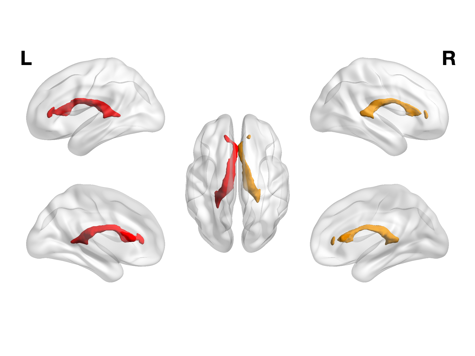
Generating Publication Figures

BrainNet Viewer (MATLAB)

Convert mgz image to NIFTI

mri_convert mri/aparc+aseg.mgz aparc+aseg.nii.gz

You can also extract specific ROIs:

c3d \
aparc+aseg.nii.gz -thresh 4 4 1 0 \
aparc+aseg.nii.gz -thresh 43 43 1 0 \
-add \
-o lateralventricles.nii.gz

How to load the program in MATLAB:

cd ('/fslhome/intj5/compute/data/KPCA/freesurfer_subjects/sub-M2PR002_ses-1/');

% Get home directory:
var = getenv('HOME');

BrainNetPath = [var, '/apps/matlab/BrainNetViewer_20191031'];
addpath(genpath(BrainNetPath));

Merge your left and right surface pial to get a participant specific image: Tools > Merge Mesh

You can load files: File > Load File

Load surface (pial or standard)
Load mapping

Option > Layout > Lateral, medial, and dorsal view
Option > Volume > ROI drawing > Custom (4,43)

R GGSEG

https://lcbc-uio.github.io/ggseg/articles/ggseg.html

To install ggseg make sure to run gcc and the latest version of R:

module load gcc
module load r/3.6_X11

Installing ggseg is a bit of a chore. Install programs and load programs in this precise order. ORDER MATTERS!

chooseCRANmirror()
install.packages("ggplot2", dependencies = TRUE)
install.packages("remotes")
remotes::install_github("LCBC-UiO/ggseg", build_vignettes = FALSE)
remotes::install_github("LCBC-UiO/ggseg3d")

library(ggseg)
library(ggseg3d)

ggseg()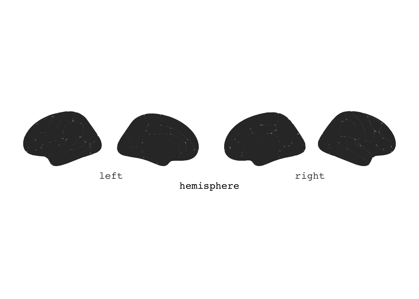

ggseg(position="stacked")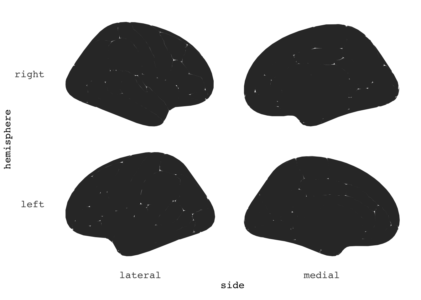

ggseg(mapping=aes(fill=region), position="stacked")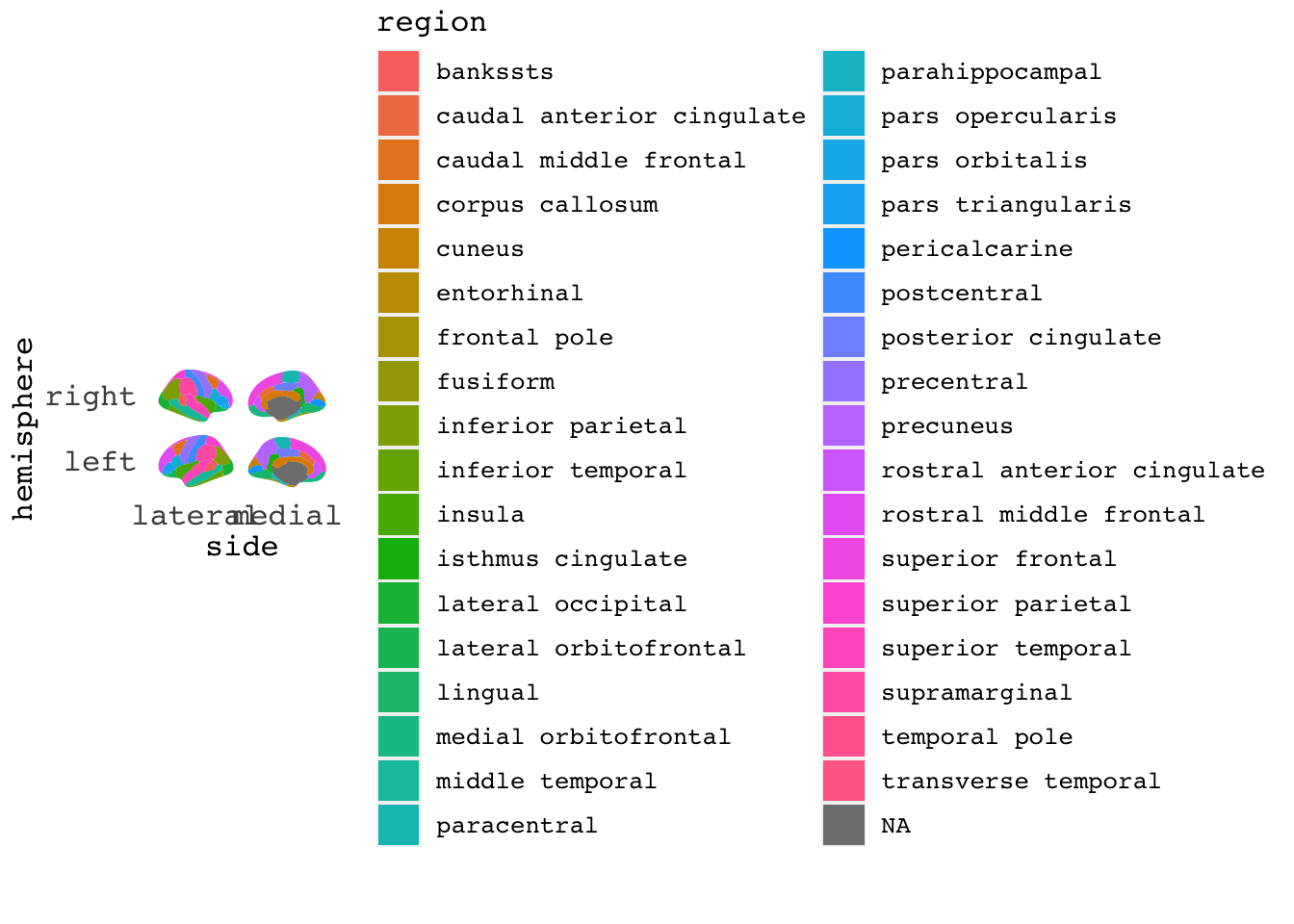

ggseg(mapping=aes(fill=region),
      position = "stacked") +
  scale_fill_brain("dk") +
  theme_void()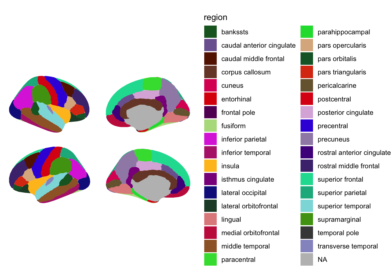

ggseg(mapping=aes(fill=region), position="stacked", show.legend = F) +
  ggtitle("Desikan-Killany cortical atlas")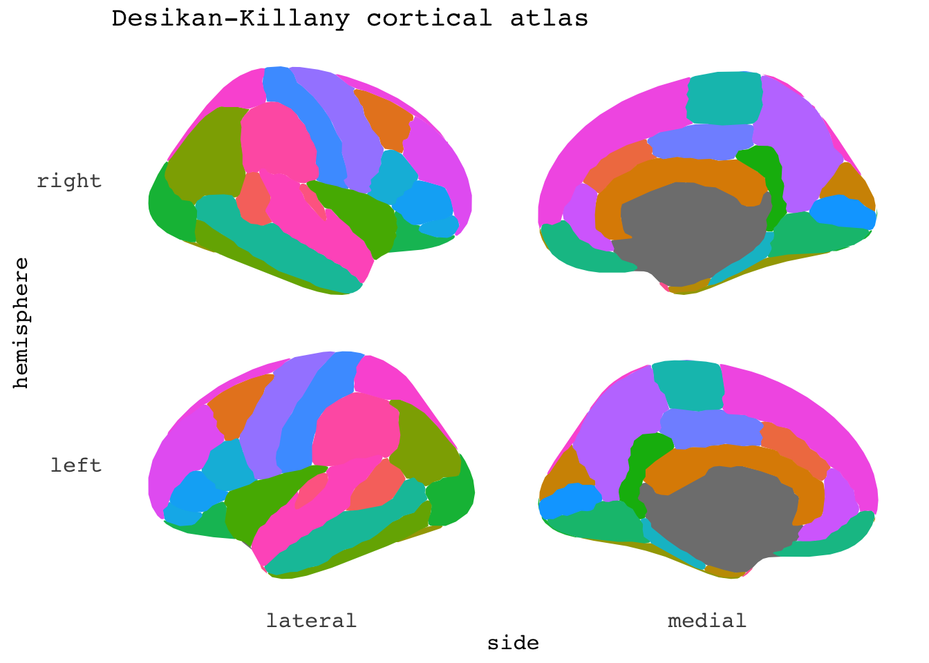

ggseg(atlas="aseg", mapping=aes(fill=region)) +
theme_void()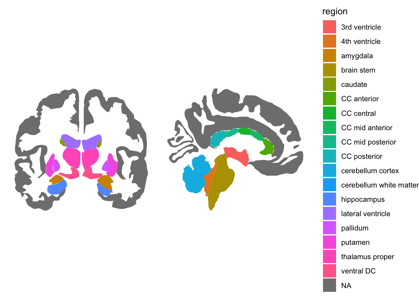

someData = data.frame(
  region = c("transverse temporal", "insula",
           "precentral","superior parietal"),
  p = sample(seq(0,.5,.001), 4),
  stringsAsFactors = FALSE)

ggseg(.data=someData, mapping=aes(fill=p))

## merging atlas and data by 'region'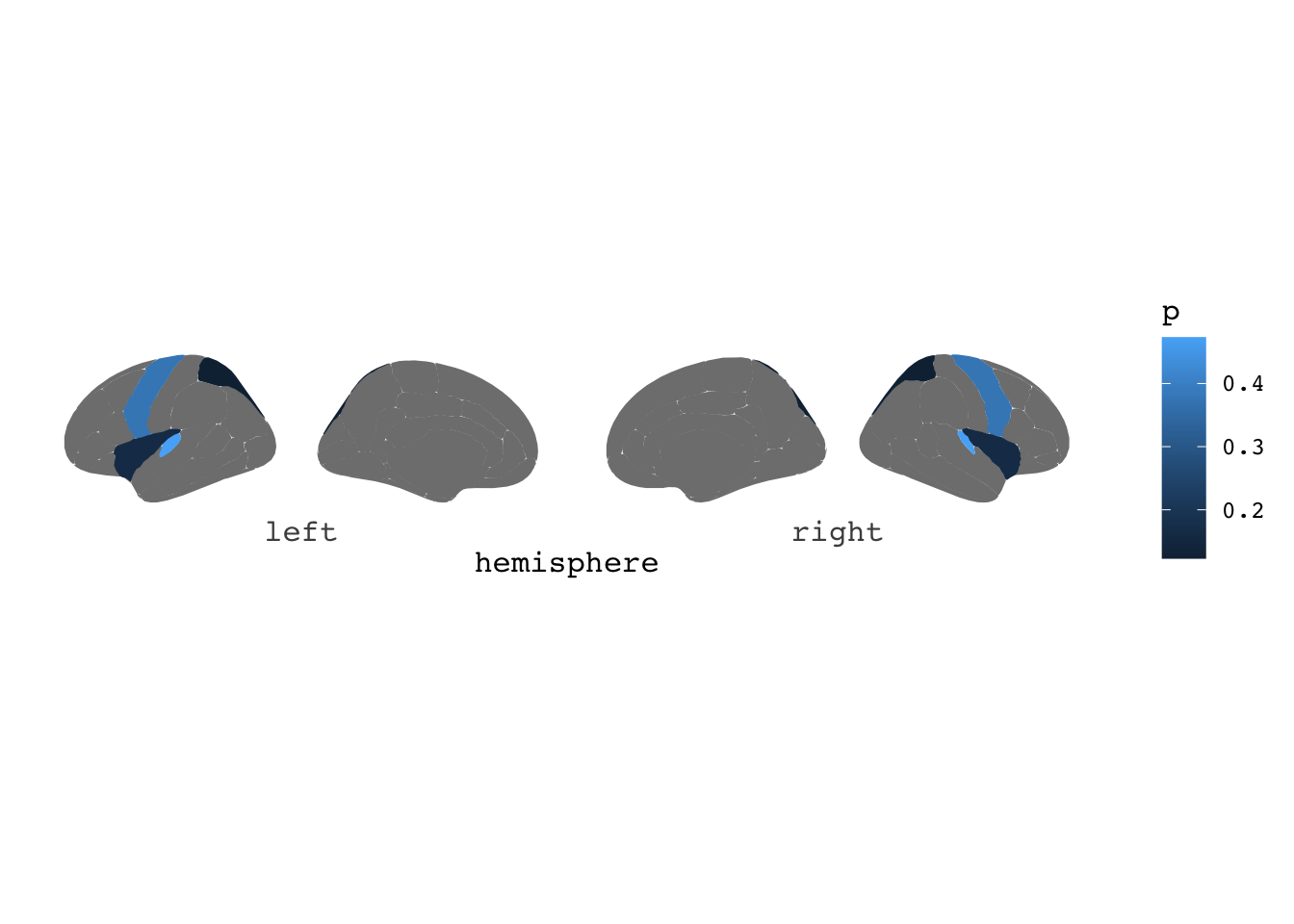

someData = data.frame(
  region = rep(c("transverse temporal", "insula", "precentral","superior parietal"), 2),
  p = sample(seq(0,.5,.001), 8),
  AgeG = c(rep("Young",4), rep("Old",4)),
  stringsAsFactors = FALSE)

someData = someData %>%
  group_by(AgeG)

ggseg(.data = someData, atlas=dk, colour="white", mapping=aes(fill=p)) +
  facet_wrap(~AgeG, ncol=1) +
  theme(legend.position = "bottom")

## merging atlas and data by 'region'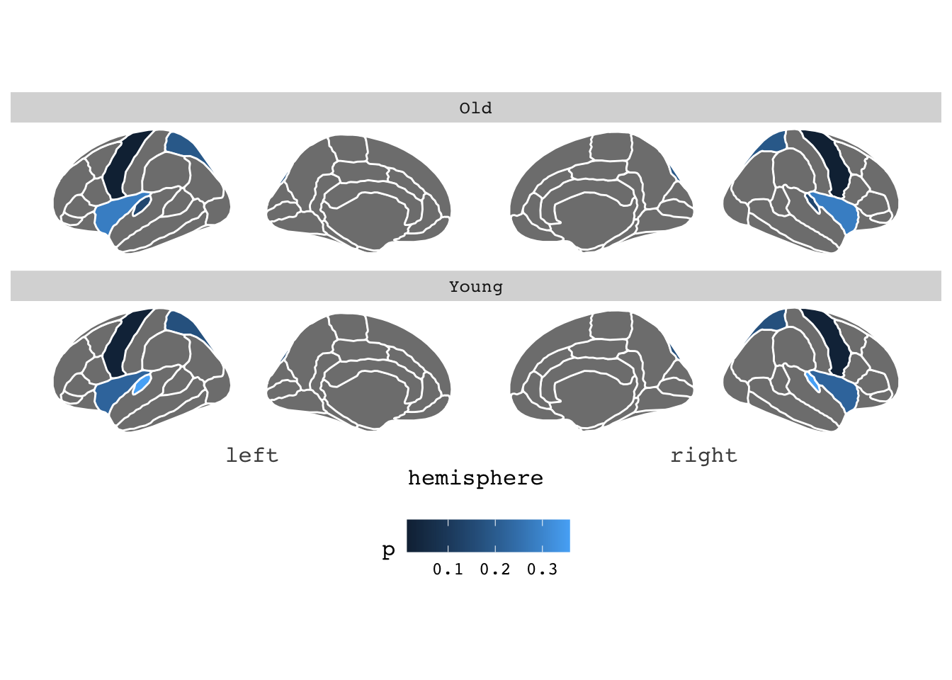

someData = data.frame(
  region = c("superior frontal", "rostral middle frontal", "caudal middle frontal", "pars opercularis",
           "pars triangularis", "pars orbitalis", "lateral orbitofrontal", "medial orbitofrontal",
           "precentral", "paracentral", "frontal pole", "superior parietal", "inferior parietal",
           "supramarginal", "postcentral", "precuneus", "superior temporal", "middle temporal",
           "inferior temporal", "bankssts", "fusiform", "transverse temporal",
           "entorhinal","temporal pole", "parahippocampal", "lateral occipital", "lingual", "cuneus",
           "pericalcarine","rostral anterior cingulate", "caudal anterior cingulate",
           "posterior cingulate","isthmus cingulate", "insula"),
  p = c(1, 1, 1, 1, 1, 1, 1, 1, 1, 1, 1, 2, 2, 2, 2, 2, 3, 3, 3, 3, 3, 3, 3, 3, 3, 4, 4, 4, 4, 5, 5, 5, 5, 6),
        stringsAsFactors = FALSE)

ggseg(position="stacked", colour="white", .data=someData, mapping=aes(fill=factor(p))) +
theme_void() +
scale_fill_manual(breaks = c("1", "2", "3", "4", "5", "6"),
                  labels = c("Frontal", "Parietal", "Temporal", "Occipital", "Cingulate", "Insula"),
                  values = c("red", "blue", "green", "purple", "yellow", "orange"),
                  na.value="grey") +
theme(legend.position = "bottom") +
labs(fill="")

## merging atlas and data by 'region'

FreeSurfer

recon-all

Euler

Subcortical Segmentation (aseg)

Volume in mm3

Cortical Parcellation (aparc)

Area in mm2

Volume in mm3

White Matter Volume in mm3

Cortical Thickness in mm

Mean Curvature

Compare Atlases

APARC Parcellations by Lobes

Hippocampus & Amygdala

Brainstem

Thalamus

Longitudinal Analyses

Unbiased Subject Template

Longitudinal Analysis

Hippocampus & Amygdala Longitudinal

Files

FreeSurfer Subjects Directory

Output Tables found on Github

Generating Publication Figures

BrainNet Viewer (MATLAB)

R GGSEG

Volume in mm³

Area in mm²

Volume in mm³

White Matter Volume in mm³