Chapter 2 Working with vectors, matrices, and arrays
2.1 Data objects in R
2.1.1 Atomic vs. recursive data objects
The analysis of data in R involves creating, naming, manipulating, and
operating on data objects using functions. Data in R are organized as
objects and have been assigned names. We have already been introduced
to several R data objects. Now we make further distinctions. Every
data object has a mode and length. The mode of an object
describes the type of data it contains and is available by using the
mode function. An object can be of mode character, numeric,
logical, list, or function.
#> [1] "character"#> [1] "numeric"#> [1] FALSE TRUE#> [1] "logical"#> [1] "list"#> [1] "list"#> [1] 25#> [1] "function"Data objects are further categorized into atomic or recursive objects. An atomic data object can only contain elements from one, and only one, of the following modes: character, numeric, or logical. Vectors, matrices, and arrays are atomic data objects. A recursive data object can contain data objects of any mode. Lists, data frames, and functions are recursive data objects. We start by reviewing atomic data objects.
A vector is a collection of like elements without
dimensions.14 The vector elements are all of the same
mode (either character, numeric, or logical). When R returns a vector
the [n] indicates the position of the element displayed to its
immediate right.
#> [1] "Pedro" "Paulo" "Maria"#> [1] 1 2 3 4 5#> [1] TRUE TRUE FALSE FALSE FALSERemember that a numeric vector can be of type double precision or integer. By default R does not use single precision numeric vectors. The vector type is not apparent by inspection (also see Table 2.1).
#> [1] 3 4 5#> [1] "double"#> [1] 3 4 5#> [1] "integer"| vector example | mode(x) |
typeof(x) |
class(x) |
|---|---|---|---|
x <- c(3, 4, 5) |
numeric |
double |
numeric |
x <- c(3L, 4L, 5L) |
numeric |
integer |
integer |
A matrix is a collection of like elements organized into a
2-dimensional (tabular) data object with r rows and c columns. We
can think of a matrix as a vector re-shaped into a \(r \times c\) table.
When R returns a matrix the [i,] indicates the ith row and
[,j] indicates the jth column.
#>      [,1] [,2]
#> [1,] "a"  "c"
#> [2,] "b"  "d"
An array is a collection of like elements organized into a
z-dimensional data object. We can think of an array as a vector
re-shaped into a \(n_1 \times n_2 \times n_3 \ldots n_z\) table. For
example, when R returns a 3-dimensional array the [i,,]
indicates the ith row and [,j,] indicates the jth column,
and “, , k” indicates the kth depth.
#> , , 1
#>
#>      [,1] [,2] [,3]
#> [1,]    1    3    5
#> [2,]    2    4    6
#>
#> , , 2
#>
#>      [,1] [,2] [,3]
#> [1,]    7    9   11
#> [2,]    8   10   12
If we try to include elements of different modes in an atomic data object, R will coerce the data object into a single mode based on the following hierarchy: character \(>\) numeric \(>\) logical. In other words, if an atomic data object contains any character element, all the elements are coerced to character.
#> [1] "hello" "4.56" "FALSE"#> [1] 4.56 0.00A recursive data object can contain one or more data objects where each object can be of any mode. Lists, data frames, and functions are recursive data objects. Lists and data frames are of mode list, and functions are of mode function (Table 2.2).
A list is a collection of data objects without any restrictions. Think of a list of length \(k\) as \(k\) “bins” in which each bin can contain any type of data object.
x <- c(1, 2, 3)                   # numeric vector
y <- c('Male', 'Female', 'Male')  # character vector
z <- matrix(1:4, 2, 2)            # numemric matrix
mylist <- list(x, y, z); mylist   # list
#> [[1]]
#> [1] 1 2 3
#>
#> [[2]]
#> [1] "Male" "Female" "Male"
#>
#> [[3]]
#> [,1] [,2]
#> [1,] 1 3
#> [2,] 2 4A data frame is a special list with a 2-dimensional (tabular) structure. Epidemiologists are very experienced working with data frames where each row usually represents data collected on individual subjects (also called records or observations) and columns represent fields for each type of data collected (also called variables).
subjno <- c(1, 2, 3, 4)
age <- c(34, 56, 45, 23)
sex <- c('Male', 'Male', 'Female', 'Male')
case <- c('Yes', 'No', 'No', 'Yes')
mydat <- data.frame(subjno, age, sex, case); mydat
#> subjno age sex case
#> 1 1 34 Male Yes
#> 2 2 56 Male No
#> 3 3 45 Female No
#> 4 4 23 Male Yes#> [1] "list"A tibble “is a modern reimagining of the data.frame, keeping what
time has proven to be effective, and throwing out what is not. Tibbles
are data.frames that are lazy and surly: they do less (i.e. they don’t
change variable names or types, and don’t do partial matching) and
complain more (e.g. when a variable does not exist). This forces you
to confront problems earlier, typically leading to cleaner, more
expressive code. Tibbles also have an enhanced print() method which
makes them easier to use with large datasets containing complex
objects.” To learn more see https://tibble.tidyverse.org.
2.1.2 Assessing the structure of data objects
| Data object | Possible mode | Default class |
|---|---|---|
| Atomic | ||
| vector | character, numeric, logical | NULL |
| matrix | character, numeric, logical | NULL |
| array | character, numeric, logical | NULL |
| Recursive | ||
| list | list | NULL |
| data frame | list | data.frame |
| function | function | NULL |
Summarized in Table 2.2 are the key attributes of
atomic and recursive data objects. Data objects can also have class
attributes. Class attributes are just a way of letting R know that an
object is ‘special,’ allowing R to use specific methods designed for
that class of objects (e.g., print, plot, and summary methods).
The class function displays the class if it exists. For our
purposes, we do not need to know any more about classes.
Frequently, we need to assess the structure of data objects. We
already know that all data objects have a mode and
length attribute. For example, let’s explore the infert data
set that comes with R. The infert data comes from a matched
case-control study evaluating the occurrence of female infertility
after spontaneous and induced abortion.
#> [1] "list"#> [1] 8At this point we know that the data object named ‘infert’ is a list
of length 8. To get more detailed information about the structure of
infert use the str function (str comes from
’str’ucture).
#> 'data.frame':    248 obs. of  8 variables:
#>  $ education     : Factor w/ 3 levels "0-5yrs","6-11yrs",..: 1 1 1 1 2 2 2 2 2 2 ...
#>  $ age           : num  26 42 39 34 35 36 23 32 21 28 ...
#>  $ parity        : num  6 1 6 4 3 4 1 2 1 2 ...
#>  $ induced       : num  1 1 2 2 1 2 0 0 0 0 ...
#>  $ case          : num  1 1 1 1 1 1 1 1 1 1 ...
#>  $ spontaneous   : num  2 0 0 0 1 1 0 0 1 0 ...
#>  $ stratum       : int  1 2 3 4 5 6 7 8 9 10 ...
#>  $ pooled.stratum: num  3 1 4 2 32 36 6 22 5 19 ...
Great! This is better. We now know that infert is a data
frame with 248 observations and 8 variables. The variable names and
data types are displayed along with their first few values. In this
case, we now have sufficient information to start manipulating and
analyzing the infert data set.
Additionally, we can extract more detailed structural information that becomes useful when we want to extract data from an object for further manipulation or analysis (Table 2.3). We will see extensive use of this when we start programming in R.
To get practice calling data from the console, enter data() to
display the available data sets in R. Then enter data(data_set)
to load a dataset. Study the examples in Table
2.3 and spend a few minutes exploring the
structure of the data sets we have loaded. To display detailed
information about a specific data set use ?data_set at the command
prompt (e.g., ?infert).
| Function | Returns |
|---|---|
str |
summary of data object structure |
attributes |
list with data object attributes |
mode |
mode of object |
typeof |
type of object; similar to mode but includes double and integer, if applicable |
length |
length of object |
class |
class of object, if it exists |
dim |
vector with object dimensions, if applicable |
nrow |
number of rows, if applicable |
ncol |
number of columns, if applicable |
dimnames |
list containing vectors of names for each dimension, if applicable |
rownames |
vector of row names of a matrix-like object |
colnames |
vector of column names of a matrix-like object |
names |
vector of names for the list (for a data frame returns field names) |
row.names |
vector of row names for a data frame |
2.2 A vector is a collection of like elements
2.2.1 Understanding vectors
A vector15 is a collection of like elements (i.e., the
elements all have the same mode). There are many ways to create
vectors (see Table 2.6). The most common way of
creating a vector is using the c function:
#> [1] 136 219 176 214 164#> [1] "Mateo" "Mark" "Luke" "Juan"#> [1] TRUE TRUE FALSE TRUE FALSEA single element is also a vector; that is, a vector of length = 1.
Try, for example, is.vector('Zoe'). In mathematics, a single
number is called a scalar; in R, it is a numeric vector of
length = 1. When we execute a math operation between a scalar and a
vector, in the background, the scalar expands to the same length as
the vector in order to execute a vectorized operation. For example,
these two calculation are equivalent:
#> [1] 50 100 150#> [1] 50 100 150A note of caution: when vector lengths differ, the shorter vector will recyle its elements to enable a vectorized operation. For example,
x <- c(3, 5); y = c(10, 20, 30, 40)
z <- x * y     # multipy vectors with different lengths
cbind(x, y, z) # display results
#> x y z
#> [1,] 3 10 30
#> [2,] 5 20 100
#> [3,] 3 30 90
#> [4,] 5 40 200In effect, x expanded from c(3, 5) to c(3, 5, 3, 5) in order to
execute a vectorized operation. This expansion of x is not apparent
from the math operation; that is, no warning was produced. Therefore,
be aware: math operations with vectors of different lengths may not
produce a warning.
2.2.1.1 Boolean queries and subsetting of vectors
In R, we use relational and logical operators (Table
2.4) and (Table
2.5) to conduct Boolean queries. Boolean
operations is a methodological workhorse of data analysis. For
example, suppose we have a vector of female movie stars and a
corresponding vector of their ages (as of January 16, 2004), and we
want to select a subset of actors based on age criteria. Let’s select
the actors who are in their 30s. This is done using logical vectors
that are created by using relational operators (<, >, <=, >=,
==, !=). Study the following example:
movie.stars <- c('Rebecca', 'Elisabeth', 'Amanda', 'Jennifer',
                 'Winona', 'Catherine', 'Reese')
ms.ages <- c(42, 40, 32, 33, 32, 34, 27)
ms.ages >= 30 # logical vector for stars with ages >=30
#> [1] TRUE TRUE TRUE TRUE TRUE TRUE FALSE#> [1] FALSE FALSE TRUE TRUE TRUE TRUE TRUE#> [1] FALSE FALSE TRUE TRUE TRUE TRUE FALSEthirtysomething <- (ms.ages >= 30) & (ms.ages < 40)
movie.stars[thirtysomething] # indexing using logical#> [1] "Amanda" "Jennifer" "Winona" "Catherine"| Operator | Description | Try these examples |
|---|---|---|
< |
Less than | pos <- c('p1', 'p2', 'p3', 'p4') |
x <- c(1, 2, 3, 4) |
||
y <- c(5, 4, 3, 2) |
||
x < y |
||
pos[x < y] |
||
> |
Greater than | x > y |
pos[x > y] |
||
<= |
Less than or equal to | x <= y |
pos[x <= y] |
||
>= |
Greater than or equal to | x >= y |
pos[x >= y] |
||
== |
Equal to | x == y |
pos[x == y] |
||
!= |
Not equal to | x != y |
pos[x != y] |
| Operator | Description | Try these examples |
|---|---|---|
! |
Element-wise NOT | x <- c(1, 2, 3, 4) |
x > 2 |
||
!(x > 2) |
||
pos[!(x > 2)] |
||
& |
Element-wise AND | (x > 1) & (x < 5) |
pos[(x > 1) & (x < 5)] |
||
| \(\mid\) | Element-wise OR | (x <= 1) \(\mid\) (x > 4) |
pos[(x <= 1) \(\mid\) (x > 4)] |
||
xor |
Exclusive OR: only TRUE if one | xx <- x <= 1 |
| or other element is true, not both | yy <- x > 4 |
|
xor(xx, yy) |
To summarize:
- Logical vectors are created using Boolean comparisons,
- Boolean comparisons are constructed using relational and logical operators
- Logical vectors are commonly used for indexing (subsetting) data objects
Before moving on, we need to be sure we understand the previous examples, then study the examples in the Table 2.4 and Table 2.5. For practice, study the examples and spend a few minutes creating simple numeric vectors, then
- generate logical vectors using relational operators,
- use these logical vectors to index the original numerical vector or another vector,
- generate logical vectors using the combination of relational and logical operators, and
- use these logical vectors to index the original numerical vector or another vector.
Notice that the element-wise exclusive or operator (xor) returns
TRUE if either comparison element is TRUE, but not if both are
TRUE. In contrast, the | returns TRUE if either or both
comparison elements are TRUE.
2.2.1.2 Integer queries and subsetting of vectors
TODO - which function
2.2.2 Creating vectors
| Function | Description | Try these examples |
|---|---|---|
c |
Concatenate a collection | x <- c(1, 2, 3, 4, 5) |
y <- c(6, 7, 8, 9, 10) |
||
z <- c(x, y) |
||
scan |
Scan a collection | xx <- scan() |
| (press enter twice | 1 2 3 4 5 |
|
| after last entry) | yy <- scan(what = '') |
|
'Javier' 'Miguel' 'Martin' |
||
xx; yy # Display vectors |
||
: |
Make integer sequence | 1:10 |
10:(-4) |
||
seq |
Sequence of numbers | seq(1, 5, by = 0.5) |
seq(1, 5, length = 3) |
||
zz <- c('a', 'b', 'c') |
||
seq(along = zz) |
||
rep |
Replicate argument | rep('Juan Nieve', 3) |
rep(1:3, 4) |
||
rep(1:3, 3:1) |
||
paste |
Paste character strings | paste(c('A','B','C'),1:3,sep='') |
Vectors are created directly, or indirectly as the result of
manipulating an R object. The c function for concatenating a
collection has been covered previously. Another, possibly more
convenient, method for collecting elements into a vector is with the
scan function.
This method is convenient because we do not need to type c,
parentheses, and commas to create the vector. The vector is created
after executing a newline twice.
To generate a sequence of consecutive integers use the :
function.
#> [1] -9 -8 -7 -6 -5 -4 -3 -2 -1 0 1 2 3 4 5 6 7 8However, the seq function provides more flexibility in
generating sequences. Here are some examples:
#> [1] 1.0 1.5 2.0 2.5 3.0 3.5 4.0 4.5 5.0#> [1] 1.000000 1.571429 2.142857 2.714286 3.285714 3.857143
#> [7] 4.428571 5.000000#> [1] 1.000000 1.571429 2.142857 2.714286 3.285714 3.857143
#> [7] 4.428571 5.000000These types of sequences are convenient for plotting mathematical equations.16 For example, suppose we wanted to plot the standard normal curve using the normal equation. For a standard normal curve \(\mu = 0\) (mean) and \(\sigma = 1\) (standard deviation)
\[\begin{equation} f(x) = \frac{1}{\sqrt{2 \pi \sigma^2}} \exp \left\{\frac{-(x - \mu)^2}{2 \sigma^2} \right\} \end{equation}\]
Here is the R code to plot this equation:
mu <- 0; sigma <- 1  # set constants
x <- seq(-4, 4, .01) # generate x values to plot
fx <- (1/sqrt(2*pi*sigma^2))*exp(-(x-mu)^2/(2*sigma^2))
plot(x, fx, type = 'l', lwd = 2)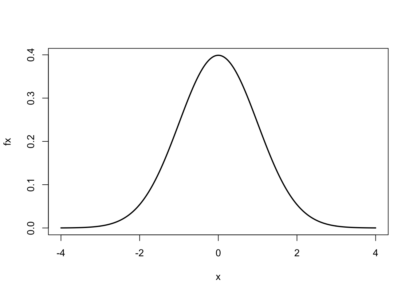
After assigning values to mu and sigma, we assigned to x a
sequence of numbers from \(-4\) to 4 by intervals of 0.01. Using the
normal curve equation, for every value of \(x\) we calculated \(f(x)\),
represented by the numeric vector fx. We then used the plot
function to plot \(x\) vs. \(f(x)\). The optional argument type='l'
produces a ‘line’ and lwd=2 doubles the line width.
The rep function is used to replicate its arguments. Study
the examples that follow:
#> [1] 5 5#> [1] 1 2 1 2 1 2 1 2 1 2#> [1] 1 1 1 1 1 2 2 2 2 2#> [1] 1 1 1 1 1 2 2 2 2 2#> [1] 1 1 1 1 1 2 2 2 2 3 3 3 4 4 5The paste function pastes character strings:
fname <- c('John', 'Kenneth', 'Sander')
lname <- c('Snow', 'Rothman', 'Greenland')
paste(fname, lname)
#> [1] "John Snow" "Kenneth Rothman" "Sander Greenland"#> [1] "var1" "var2" "var3" "var4" "var5" "var6" "var7"Indexing (subsetting) an object often results in a vector. To
preserve the dimensionality of the original object use the
drop option.
#>      [,1] [,2] [,3] [,4]
#> [1,]    1    3    5    7
#> [2,] 2 4 6 8#> [1] 2 4 6 8#> [,1] [,2] [,3] [,4]
#> [1,] 2 4 6 8Up to now we have generated vectors of known numbers or character strings. On occasion we need to generate random numbers or draw a sample from a collection of elements. First, sampling from a vector returns a vector:
#> [1] "T" "H" "H" "T" "H" "T" "T" "T"#> [1] 1 3 2 2 5 3 6 5 3 4Second, generating random numbers from a probability distribution returns a vector:
#> [1] 26 25 21 29 22 22 27 27 29 27#> [1] -0.9132501 1.2581499 -0.6512095 0.3383909 -0.2863969There are additional ways to create vectors. To practice creating
vectors study the examples in Table 2.6 and spend a few
minutes creating simple vectors. If we need help with a function
remember enter ?function_name or help(function_name).
Finally, notice that we can use vectors as arguments to functions:
2.2.3 Naming vectors
Each element of a vector can be labeled with a name at the time the vector is created or later. The first way of naming vector elements is when the vector is created:
#> chol  sbp  dbp  age
#>  234  148   78   54
The second way is to create a character vector of names and then
assign that vector to the numeric vector using the names
function:
#> [1] 234 148 78 54#> chol sbp dbp age
#> 234 148 78 54The names function, without an assignment, returns the
character vector of names, if it exist. This character vector can be
used to name elements of other vectors.
#> [1] "chol" "sbp" "dbp" "age"#> [1] 250 184 90 45#> chol sbp dbp age
#> 250 184 90 45The unname function removes the element names from a vector:
#> [1] 250 184 90 45For practice study the examples in Table 2.7 and spend a few minutes creating and naming simple vectors.
| Function | Description | Try these examples |
|---|---|---|
c |
Name elements at creation | x <- c(a = 1, b = 2, c = 3) |
names |
Name elements by assignment; | y <- 1:3 |
| Returns names if they exist | names(y) <- c('a', 'b', 'c') |
|
names(y) # return names |
||
unname |
Remove names (if they exist) | y <- unname(y) |
names(y) <- NULL #equivalent |
2.2.4 Indexing (subsetting) vectors
Indexing a vector is subsetting or extracting elements from a vector. A vector is indexed by position, by name (if it exist), or by logical value (TRUE vs FALSE). Positions are specified by positive or negative integers.
#> sbp age
#> 148 54#> chol dbp
#> 234 78Although indexing by position is concise, indexing by name (when the names exists) is better practice in terms of documenting our code. Here is an example:
#> sbp age
#> 148  54
A logical vector indexes the positions that corresponds to the TRUEs. Here is an example:
#>  chol   sbp   dbp   age
#> TRUE FALSE TRUE TRUE#> chol dbp age
#> 234 78 54Any expression that evaluates to a valid vector of integers, names, or logicals can be used to index a vector.
#> [1] 1 1 3 4 4 3 1#> chol chol dbp age age dbp chol
#> 234 234 78 54 54 78 234#> [1] "chol" "chol" "age" "sbp" "dbp" "dbp" "age"#> chol chol age sbp dbp dbp age
#> 234 234 54 148 78 78 54Notice that when we indexed by position or name we indexed the same position repeatly. This will not work with logical vectors. In the example that follows NA means ‘not available.’
#> [1] FALSE TRUE TRUE FALSE TRUE FALSE FALSE#> sbp dbp <NA>
#> 148 78 NAWe have already seen that a vector can be indexed based on the characteristics of another vector.
kid <- c('Tomasito', 'Irene', 'Luisito', 'Angelita', 'Tomas')
age <- c(8, NA, 7, 4, NA)
age <= 7                    # produces logical vector
#> [1] FALSE NA TRUE TRUE NA#> [1] NA "Luisito" "Angelita" NA#> [1] "Tomasito" "Luisito" "Angelita"#> [1] "Luisito" "Angelita"In this example, NA represents missing data. The
is.na function returns a logical vector with s
at NA positions. To generate a logical vector to index values that are
not missing use !is.na.
For practice study the examples in Table 2.8 and spend a few minutes creating, naming, and indexing simple vectors.
| Indexing | Try these examples |
|---|---|
| By logical | x < 100 |
x[x < 100] |
|
(x < 150) & (x > 70) |
|
bp <- (x < 150) & (x > 70) |
|
x[bp] |
|
| By position | x <- c(chol = 234, sbp = 148, dbp = 78) |
x[2] # positions to include |
|
x[c(2, 3)] |
|
x[-c(1, 3)] # positions to exclude |
|
x[which(x<100)] |
|
| By name (if exists) | x['sbp'] |
x[c('sbp', 'dbp')] |
|
| Unique values | samp <- sample(1:5, 25, replace = TRUE) |
unique(samp) |
|
| Duplicated values | duplicated(samp) # generates logical |
samp[duplicated(samp)] |
2.2.4.1 The which function
A Boolean operation that returns a logical vector contains
TRUE values where the condition is true. To identify the
position of each TRUE value we use the which
function. For example, using the same data above:
#> [1] 3 4#> [1] "Luisito" "Angelita"Notice that is was unnecessary to remove the missing values.
2.2.5 Replacing vector elements (by indexing and assignment)
If a vector element can be indexed, it can be replaced. Therefore, to replace vector elements we combine indexing and assignment. Any elements of a vector that can be indexed can be replaced. Replacing vector elements is one method of recoding a variable. In this example, we recode a vector of ages into age categories:
age <- sample(0:100, 1000, replace = TRUE) # create vector
agecat <- age # copy vector
agecat[age<15] <- '<15'
agecat[age>=15 & age<25] <- '15-24'
agecat[age>=25 & age<45] <- '25-44'
agecat[age>=45 & age<65] <- '45-64'
agecat[age>=65] <- '65+'
table(agecat)
#> agecat
#> <15 15-24 25-44 45-64 65+
#> 153 97 193 198 359First, we made a copy of the numeric vector age and
named it agecat. Then, we replaced elements of
agecat with character strings for each age category, creating
a character vector.
For practice study the examples in Table 2.9 and spend a few minutes replacing vector elements.
| Replacing | Try these examples |
|---|---|
| By logical | x[x<100] |
x[x<100] <- NA; x |
|
| By position | x <- c(chol = 234, sbp = 148, dbp = 78) |
x[1] |
|
x[1] <- 250; x |
|
| By name (if exists) | x['sbp'] |
x['sbp'] <- 150; x |
2.2.6 Operating on vectors
Operating on vectors is very common in epidemiology and statistics. In this section we cover common operations on single vectors (Table 2.10) and multiple vectors (Table 2.11).
2.2.6.1 Operating on single vectors
| Function | Description | Function | Description | |
|---|---|---|---|---|
sum |
summation | rev |
reverse order | |
cumsum |
cumulative sum | order |
order | |
diff |
x[i+1]-x[i] |
sort |
sort | |
prod |
product | rank |
rank | |
cumprod |
cumulative product | sample |
random sample | |
mean |
mean | quantile |
percentile | |
median |
median | var |
variance, covariance | |
min |
minimum | sd |
standard deviation | |
max |
maximum | table |
tabulate character vector | |
range |
range | xtabs |
tabulate factor vector |
First, we focus on operating on single numeric vectors (Table 2.10). This also gives us the opportunity to see how common mathematical notation is translated into simple R code.
To sum elements of a numeric vector \(x\) of length \(n\),
(\(\sum_{i=1}^{n}{x_i}\)), use the sum function:
#> [1] 12.15179To calculate a cumulative sum of a numeric vector \(x\) of length \(n\),
(\(\sum_{i=1}^{k}{x_i}\), for \(k=1,\ldots,n\)), use the cumsum
function which returns a vector:
#> [1] 2 2 2 2 2 2 2 2 2 2#> [1] 2 4 6 8 10 12 14 16 18 20To multiply elements of a numeric vector \(x\) of length \(n\),
(\(\prod_{i=1}^{n}{x_i}\)), use the prod function:
#> [1] 40320To calculate the cumulative product of a numeric vector \(x\) of length
\(n\), (\(\prod_{i=1}^{k}{x_i}\), for \(k=1,\ldots,n\)), use the
cumprod function:
#> [1] 1 2 6 24 120 720 5040 40320To calculate the mean of a numeric vector \(x\) of length \(n\),
(\(\frac{1}{n} \sum_{i=1}^{n}{x_i}\)), use the sum and
length functions, or use the mean function:
#> [1] 0.04400498#> [1] 0.04400498To calculate the sample variance of a numeric vector \(x\) of length
\(n\), use the sum, mean, and length
functions, or, more directly, use the var function.
\[\begin{equation} S_X^2 = \frac{1}{n-1} \left[ \sum_{i = 1}^n{(x_i - \bar{x})^2} \right] \end{equation}\]
#> [1] 0.9444244#> [1] 0.9444244This example illustrates how we can implement a formula in R using
several functions that operate on single vectors (sum,
mean, and length). The var function, while
available for convenience, is not necessary to calculate the sample
variance.
When the var function is applied to two numeric vectors, \(x\)
and \(y\), both of length \(n\), the sample covariance is calculated:
\[\begin{equation} S_{XY} = \frac{1}{n-1} \left[ \sum_{i = 1}^n{(x_i - \bar{x}) (y_i - \bar{y})} \right] \end{equation}\]
#> [1] -0.2808559#> [1] -0.2808559The sample standard deviation, of course, is just the square root of
the sample variance (or use the sd function):
\[\begin{equation} S_X = \sqrt{\frac{1}{n-1} \left[ \sum_{i = 1}^n{(x_i - \bar{x})^2} \right]} \end{equation}\]
#> [1] 1.156758#> [1] 1.156758To sort a numeric or character vector use the sort function.
#> [1] 4 7 8However, to sort one vector based on the ordering of another vector
use the order function.
#> [1] "Angela" "Luis" "Tomas"#> [1] 2 3 1Notice that the order function does not return the data, but rather
indexing integers in new positions for sorting the vector age or
another vector. For example, order(ages) returned the integer
vector c(2, 3, 1) which means “move the 2nd element (age = 4) to the
first position, move the 3rd element (age = 7) to the second position,
and move the 1st element (age = 8) to the third position.” Verify
that sort(ages) and ages[order(ages)] are equivalent.
To sort a vector in reverse order combine the rev and
sort functions.
#> [1] 1 3 3 5 12 14#> [1] 14 12 5 3 3 1In contrast to the sort function, the rank
function gives each element of a vector a rank score but does not sort
the vector.
#> [1] 5.0 2.5 6.0 2.5 4.0 1.0The median of a numeric vector is that value which puts 50% of the
values below and 50% of the values above, in other words, the 50%
percentile (or 0.5 quantile). For example, the median of c(4, 3, 1, 2, 5) is 3. For a vector of even length, the middle values
are averaged: the median of c(4, 3, 1, 2) is 2.5. To get the
median value of a numeric vector use the median or
quantile function.
#> [1] 39#> 50%
#> 39To return the minimum value of a vector use the min function;
for the maximum value use the max function. To get both the
minimum and maximum values use the range function.
#> [1] 20#> [1] 20#> [1] 77#> [1] 77#> [1] 20 77#> [1] 20 77To sample from a vector of length \(n\), with each element having a
default sampling probability of \(1/n\), use the sample
function. Sampling can be with or without replacement (default). If
the sample size is greater than the length of the vector, then
sampling must occur with replacement.
#> [1] "H" "T" "H" "H" "T" "H" "H" "H" "T" "T"#> [1] 86 69 29 76 100 83 44 25 39 94 66 40 79 80 422.2.6.2 Operating on multiple vectors
| Function | Description |
|---|---|
c |
Concatenates into vectors |
append |
Appends a vector to another vector |
cbind |
Column-bind vectors or matrices |
rbind |
Row-bind vectors or matrices |
table |
Creates contingency table from 2 or more vectors |
xtabs |
Creates contingency table from 2 or more factors in a data frame |
ftable |
Creates flat contingency table from 2 or more vectors |
outer |
Outer product |
tapply |
Applies a function to strata of a vector |
<, > |
Relational operators |
<=, >= |
|
==, != |
|
!, |, xor |
Logical operators |
Next, we review selected functions that work with one or more vectors. Some of these functions manipulate vectors and others facilitate numerical operations.
In addition to creating vectors, the c function can be used
to append vectors.
#> [1] 6 7 8 9 10 20 21 22 23 24The append function also appends vectors; however, one can
specify at which position.
#> [1] 6 7 8 9 10 20 21 22 23 24#> [1] 6 7 20 21 22 23 24 8 9 10In contrast, the cbind and rbind functions concatenate vectors
into a matrix. During the outbreak of severe acute respiratory
syndrome (SARS) in 2003, a patient with SARS potentially exposed 111
passengers on board an airline flight. Of the 23 passengers that sat
‘close’ to the index case, 8 developed SARS; among the 88 passengers
that did not sit ‘close’ to the index case, only 10 developed SARS
[8]. Now, we can bind 2 vectors to create a \(2 \times 2\) table (matrix).
case <- c(exposed = 8, unexposed = 10)
noncase <- c(exposed = 15, unexposed = 78)
cbind(case, noncase)
#> case noncase
#> exposed 8 15
#> unexposed 10 78#> exposed unexposed
#> case 8 10
#> noncase 15 78For the example that follows, let’s recreate the SARS data as two character vectors.
outcome <- c(rep("case", 8 + 10), rep("noncase", 15 + 78))
tmp <- c("exposed", "unexposed")
exposure <- c(rep(tmp, c(8, 10)), rep(tmp, c(15, 78)))
cbind(exposure, outcome)[1:4, ]  # display 4 rows
#> exposure outcome
#> [1,] "exposed" "case"
#> [2,] "exposed" "case"
#> [3,] "exposed" "case"
#> [4,] "exposed" "case"Now, use the table function to cross-tabulate one or more
vectors.
#>          exposure
#> outcome   exposed unexposed
#>   case          8        10
#>   noncase      15        78
The ftable function creates a flat contingency table from one
or more vectors.
#>         exposure exposed unexposed
#> outcome
#> case                   8        10
#> noncase               15        78
This will come in handy later when we want to display a 3 or more dimensional table as a ‘flat’ 2-dimensional table.
The outer function applies a function to every combination of
elements from two vectors. For example, create a multiplication table
for the numbers 1 to 5.
#>      [,1] [,2] [,3] [,4] [,5]
#> [1,]    1    2    3    4    5
#> [2,]    2    4    6    8   10
#> [3,]    3    6    9   12   15
#> [4,]    4    8   12   16   20
#> [5,]    5   10   15   20   25
The tapply function applies a function to strata of a vector
that is defined by one or more ‘indexing’ vectors. For example, to
calculate the mean age of females and males:
age <- c(23, 45, 67, 88, 22, 34, 80, 55, 21, 48)
sex <- c("M", "F", "M", "F", "M", "F", "M", "F", "M", "F")
tapply(X = age, INDEX = sex, FUN = mean)
#> F M
#> 54.0 42.6#> F M
#> 54.0 42.6The tapply function is an important and versatile function
because it allows us to apply any function that can be applied
to a vector, to be applied to strata of a vector. Moveover, we can
use our user-created functions as well.
2.2.7 Converting vectors into factors (categorical variables)
The Williams Institute recommends a two-step approach for asking survey questions for gender identity [9]:
- [
sex] What sex were you assigned at birth, on your original birth certificate? (select one)
\(\bigcirc\) Male
\(\bigcirc\) Female
- [
gender] How do you describe yourself? (select one)
\(\bigcirc\) Male
\(\bigcirc\) Female
\(\bigcirc\) Transgender
\(\bigcirc\) Do not identify as female, male, or transgender
Suppose you conduct a survey of 100 subjects and the gender variable
is represented by a character vector. Here is the tabulation of your data:
#> [1] "Male" "Male" "Male" "Male" "Female"#> gender
#> Female Male
#> 49 51What is wrong with this tabulation? The tabulation does not have
all the possible reponse levels (“Female”, “Male”, “Transgender”,
“Neither.FMT”). This is because the first 100 respondents identified
only as female and male. The character vector only contains the actual
reponses without keeping track of the possible responses.
To remedy this we use the factor function to convert vectors into a
categorical variable that can keep track of possible response
levels. Factors is how R manages categorical variables.
gender.fac <- factor(gender, levels = c('Female','Male',
                     'Transgender', 'Neither.FMT'))
gender.fac[1:5]   # display first five
#> [1] Male Male Male Male Female
#> Levels: Female Male Transgender Neither.FMT#> gender.fac
#> Female Male Transgender Neither.FMT
#> 49 51 0 0How does the display of factors differ from the display of character vectors? This was our first introduction to factors. Later, we cover factors in more detail.
Note: factors are actually integer (numeric) vectors with labels
called levels. Try unclass(gender.fac) followed by
table(unclass(gender.fac)).
2.3 A matrix is a 2-dimensional table of like elements
2.3.1 Understanding matrices
A matrix is a 2-dimensional table of like elements. Matrix elements can be either numeric, character, or logical. Contingency tables in epidemiology are represented in R as numeric matrices or arrays. An array is the generalization of matrices to 3 or more dimensions (commonly known as stratified tables). We cover arrays later, for now we will focus on 2-dimensional tables.
Consider the \(2\times 2\) table of crude data in Table 2.12 [10]. In this randomized clinical trial (RCT), diabetic subjects were randomly assigned to receive either tolbutamide, an oral hypoglycemic drug, or placebo. Because this was a prospective study we can calculate risks, odds, a risk ratio, and an odds ratio. We will do this using R as a calculator.
| Treatment | ||
|---|---|---|
| Outcome status | Tolbutamide | Placebo |
| Deaths | 30 | 21 |
| Survivors | 174 | 184 |
dat <- matrix(c(30, 174, 21, 184), 2, 2)
rownames(dat) <- c('Deaths', 'Survivors')
colnames(dat) <- c('Tolbutamide', 'Placebo')
coltot <- apply(dat, 2, sum)   #column totals
risks <- dat['Deaths', ]/coltot
risk.ratio <- risks/risks[2]   #risk ratio
odds <- risks/(1 - risks)
odds.ratio <- odds/odds[2]     #odds ratio
dat                            # display results
#> Tolbutamide Placebo
#> Deaths 30 21
#> Survivors 174 184#> Tolbutamide Placebo
#> risks 0.1470588 0.1024390
#> risk.ratio 1.4355742 1.0000000
#> odds 0.1724138 0.1141304
#> odds.ratio 1.5106732 1.0000000Now let’s review each line briefly to understand the analysis in more detail.
We used the rownames and the colnames
functions to assign row and column names to the matrix dat.
The row names and the column names are both character vectors.
We used the apply function to sum the columns; it
is a versatile function for applying any function to matrices or
arrays. The second argument is the MARGIN option: in this
case, MARGIN=2, meaning apply the sum function to
the columns. To sum the rows, set MARGIN=1.
Using the definition of the odds, we calculated the odds of death for each treatment group. Then we calculated the odds ratios using the placebo group as the reference.
Finally, we display the dat table we created. We
also created a table of results by row binding the vectors using the
rbind function.
In the sections that follow we will cover the necessary concepts to make the previous analysis routine.
2.3.2 Creating matrices
There are several ways to create matrices (Table 2.13). In general, we create or use matrices in the following ways:
- Contingency tables (cross tabulations)
- Spreadsheet calculations and display
- Collecting results into tabular form
- Results of 2-variable equations
| Function | Description | Try these examples |
|---|---|---|
cbind |
Column-bind | x <- 1:3; y <- 3:1; cbind(x, y) |
rbind |
Row-bind vectors | rbind(x, y) |
matrix |
Generates matrix | matrix(1:4, nrow=2, ncol=2) |
dim |
Assign dimensions | mtx2 <- 1:4 |
dim(mtx2) <- c(2, 2) |
||
table |
Cross-tabulate | table(infert$educ, infert$case) |
xtabs |
Cross-tabulate | xtabs(~education + case, data = infert) |
ftable |
Creates 2-D flat table | ftable(infert$educ, infert$spont, infert$case) |
array |
Creates 2-D array | array(1:4, dim = c(2, 2)) |
as.matrix |
Coercion | as.matrix(1:3) |
outer |
Outer product | outer(1:5, 1:5, '*') |
x[r,,] |
Indexing an array | x <- array(1:8, c(2, 2, 2)) |
x[,c,] |
x[1, , ] |
|
x[,,d] |
x[ ,1, ] |
|
x[ , ,1] |
2.3.2.1 Contingency tables (cross tabulations)
In the previous section we used the matrix function to create
the \(2 \times 2\) table for the UGDP clinical trial:
dat <- matrix(c(30, 174, 21, 184), 2, 2)
rownames(dat) <- c('Deaths', 'Survivors')
colnames(dat) <- c('Tolbutamide', 'Placebo'); dat#> Tolbutamide Placebo
#> Deaths 30 21
#> Survivors 174 184Alternatively, we can create a 2-way contingency table using the
table function with fields from a data set;
#> [1] "Status" "Treatment" "Agegrp"#>
#> Placebo Tolbutamide
#> Death 21 30
#> Survivor 184 174Alternatively, the xtabs function cross tabulates using a
formula interface. An advantage of this function is that the field
names are included.
#>           Treatment
#> Status     Placebo Tolbutamide
#>   Death         21          30
#>   Survivor     184         174
Finally, a multi-dimensional contingency table can be presented as a
2-dimensional flat contingency table using the ftable
function. Here we stratify the above table by the variable
Agegrp.
#> , , Agegrp = <55
#>
#>           Treatment
#> Status     Placebo Tolbutamide
#>   Death          5           8
#>   Survivor     115          98
#>
#> , , Agegrp = 55+
#>
#>           Treatment
#> Status     Placebo Tolbutamide
#>   Death         16          22
#> Survivor 69 76#> Agegrp <55 55+
#> Status Treatment
#> Death Placebo 5 16
#> Tolbutamide 8 22
#> Survivor Placebo 115 69
#> Tolbutamide 98 76However, notice that ftable, while preserving the
order of the variables, does provide the equivalent, namely,
Status vs. Treatment, by Agegrp. We can
fix this by reversing the order of the variables within the
xtabs function:
#>                 Treatment Placebo Tolbutamide
#> Agegrp Status
#> <55    Death                    5           8
#>        Survivor               115          98
#> 55+    Death                   16          22
#>        Survivor                69          76
2.3.2.2 Spreadsheet calculations and display
Matrices are commonly used to display spreadsheet-like calculations. In fact, a very efficient way to learn R is to use it as our spreadsheet. For example, assuming the rate of seasonal influenza infection is 10 infections per 100 person-years, let’s calculate the individual cumulative risk of influenza infection at the end of 1, 5, and 10 years. Assuming no competing risk, we can use the exponential formula:
\[\begin{equation} R(0, t) = 1 - e^{-\lambda t} \end{equation}\]
where , \(\lambda\) = infection rate, and \(t\) = time.
lamb <- 10/100
years <- c(1, 5, 10)
risk <- 1 - exp(-lamb*years)
cbind(rate = lamb, years, cumulative.risk = risk) # display
#> rate years cumulative.risk
#> [1,] 0.1 1 0.09516258
#> [2,] 0.1 5 0.39346934
#> [3,] 0.1 10 0.63212056Therefore, the cumulative risk of influenza infection after 1, 5, and 10 years is 9.5%, 39%, and 63%, respectively.
2.3.2.3 Collecting results into tabular form
A 2-way contingency table from the table or xtabs
functions does not have margin totals. However, we can construct a
numeric matrix that includes the totals. Using the UGDP data again,
dat2 <- read.table('~/data/ugdp.txt', header = TRUE, sep = ',')
tab2 <- xtabs(~Status + Treatment, data = dat2)
rowt <- tab2[, 1] + tab2[, 2]
tab2a <- cbind(tab2, Total = rowt)
colt <- tab2a[1, ] + tab2a[2, ]
tab2b <- rbind(tab2a, Total = colt)
tab2b
#> Placebo Tolbutamide Total
#> Death 21 30 51
#> Survivor 184 174 358
#> Total 205 204 409This table (tab2b) is primarily for display
purposes.
2.3.2.4 Results of 2-variable equations
When we have an equation with 2 variables, we can use a matrix to display the answers for every combination of values contained in both variables. For example, consider this equation:
\[\begin{equation} z = x y \end{equation}\]
And suppose \(x = \{1, 2, 3, 4, 5 \}\) and \(y = \{6, 7, 8, 9, 10 \}\).
Here’s the long way to create a matrix for this equation:
x <- 1:5; y <- 6:10
z <- matrix(NA, 5, 5) #create empty matrix of missing values
for(i in 1:5){
    for(j in 1:5){
        z[i, j] <- x[i]*y[j]
    }
}
rownames(z) <- x; colnames(z) <- y; z
#> 6 7 8 9 10
#> 1 6 7 8 9 10
#> 2 12 14 16 18 20
#> 3 18 21 24 27 30
#> 4 24 28 32 36 40
#> 5 30 35 40 45 50Okay, but the outer function is much better for this task:
#>    6  7  8  9 10
#> 1  6  7  8  9 10
#> 2 12 14 16 18 20
#> 3 18 21 24 27 30
#> 4 24 28 32 36 40
#> 5 30 35 40 45 50In fact, the outer function can be used to calculate the
‘surface’ for any 2-variable equation (more on this later).
2.3.3 Naming matrix components
We have already seen several examples of naming components of a matrix. Table 2.14 summarizes the common ways of naming matrix components. The components of a matrix can be named at the time the matrix is created, or they can be named later. For a matrix, we can provide the row names, column names, and field names.
| Function | Try these examples |
|---|---|
matrix |
# name rows and columns only |
dat <- matrix(c(178, 79, 1411, 1486), 2, 2, |
|
dimnames = list(c('TypeA','TypeB'), c('Y','N'))) |
|
# name rows, columns, and fields |
|
dat <- matrix(c(178, 79, 1411, 1486), 2, 2, |
|
dimnames = list(Behavior = c('TypeA','TypeB'), |
|
'Heart attack' = c('Y','N'))) |
|
rownames |
dat <- matrix(c(178, 79, 1411, 1486), 2, 2) |
rownames(dat) <- c('TypeA','TypeB') |
|
colnames |
colnames(dat) <- c('Y','N') # col names |
dimnames |
# name rows and columns only |
dat <- matrix(c(178, 79, 1411, 1486), 2, 2) |
|
dimnames(dat) <- list(c('TypeA','TypeB'), c('Y','N')) |
|
# name rows, columns, and fields |
|
dat <- matrix(c(178, 79, 1411, 1486), 2, 2) |
|
dimnames(dat) <- list(Behavior = c('TypeA','TypeB'), |
|
'Heart attack' = c('Y','N')) |
|
names |
# add field to row \& col names |
`dat <- matrix(c(178, 79, 1411, 1486), 2, 2, |
|
dimnames = list(c('TypeA','TypeB'), c('Y','N'))) |
|
names(dimnames(dat)) <- c('Behavior', 'Heart attack') |
For example, the UGDP clinical trial \(2 \times 2\) table can be created de novo:
ugdp2x2 <- matrix(c(30, 174, 21, 184), 2, 2,
              dimnames = list(Outcome = c('Deaths', 'Survivors'),
              Treatment = c('Tolbutamide', 'Placebo')))
ugdp2x2
#> Treatment
#> Outcome Tolbutamide Placebo
#> Deaths 30 21
#> Survivors 174 184In the ‘Treatment’ field, the possible values, ‘Tolbutamide’ and ‘Placebo,’ are the column names. Similarly, in the ‘Status’ field, the possible values, ‘Death’ and ‘Survivor,’ are the row names.
If a matrix does not have field names, we can add them after the fact,
but we must use the names and dimnames
functions together. Having field names is necessary if the row and
column names are not self-explanatory, as this example illustrates.
y <- matrix(c(30, 174, 21, 184), 2, 2)
rownames(y) <- c('Yes', 'No'); colnames(y) <- c('Yes', 'No')
y # labels not informative; add field names next#> Yes No
#> Yes 30 21
#> No 174 184#> Tolbutamide
#> Death Yes No
#> Yes 30 21
#> No 174 184Study and test the examples in Table 2.14.
2.3.4 Indexing (subsetting) a matrix
Similar to vectors, a matrix can be indexed by position, by name, or by logical. Study and practice the examples in (Table 2.15). An important skill to master is indexing rows of a matrix using logical vectors.
| Indexing | Try these examples |
|---|---|
| By logical | dat[, 1] > 100 |
dat[dat[, 1] > 100, ] |
|
dat[dat[, 1] > 100, , drop = FALSE] |
|
| By position | dat <- matrix(c(178, 79, 1411, 1486), 2, 2) |
dimnames(dat) <- list(Behavior = c('Type A', |
|
'Type B'), 'Heart attack' = c('Yes', 'No')) |
|
dat[1, ] |
|
dat[1,2] |
|
dat[2, , drop = FALSE] |
|
| By name (if exists) | dat['Type A', ] |
dat['Type A', 'Type B'] |
|
dat['Type B', , drop = FALSE] |
Consider the following matrix of data, and suppose I want to select the rows for subjects age less than 60 and systolic blood pressure less than 140.
age <- c(45, 56, 73, 44, 65)
chol <- c(145, 168, 240, 144, 210)
sbp <- c(124, 144, 150, 134, 112)
dat <- cbind(age, chol, sbp); dat#> age chol sbp
#> [1,] 45 145 124
#> [2,] 56 168 144
#> [3,] 73 240 150
#> [4,] 44 144 134
#> [5,] 65 210 112#> [1] TRUE TRUE FALSE TRUE FALSE#> [1] TRUE FALSE FALSE TRUE TRUE#> [1] TRUE FALSE FALSE TRUE FALSE#> age chol sbp
#> [1,] 45 145 124
#> [2,] 44 144 134Notice that the tmp logical vector is
the intersection of the logical vectors separated by the logical
operator &.
2.3.5 Replacing matrix elements
Remember, replacing matrix elements is just indexing plus assignment: anything that can be indexed can be replaced. Study and practice the examples in (Table 2.16).
| Replacing | Try these examples |
|---|---|
| By logical | qq <- dat[, 1] < 100 # logic vector |
dat[qq, ] <- 99; dat |
|
dat[dat[, 1] < 100, ] <- c(79, 1486); dat |
|
| By position | dat <- matrix(c(178, 79, 1411, 1486), 2, 2) |
dimnames(dat) <- list(c('Type A','Type B'), |
|
c('Yes','No')) |
|
dat[1, ] <- 99; dat |
|
| By name (if exists) | dat['Type A', ] <- c(178, 1411); dat |
2.3.6 Operating on a matrix
In epidemiology books, authors have preferences for displaying contingency tables. Software packages have default displays for contingency tables. In practice, we may need to manipulate a contingency table to facilitate further analysis. Consider the following 2-way table:
tab <- matrix(c(30, 174, 21, 184), 2, 2, dimnames =
list(Outcome= c('Deaths', 'Survivors'),
Treatment = c('Tolbutamide', 'Placebo'))); tab#> Treatment
#> Outcome Tolbutamide Placebo
#> Deaths 30 21
#> Survivors 174 184We can transpose the matrix using the t function.
#> Outcome
#> Treatment Deaths Survivors
#> Tolbutamide 30 174
#> Placebo 21 184We can reverse the order of the rows and/or columns.
#> Treatment
#> Outcome Tolbutamide Placebo
#> Survivors 174 184
#> Deaths 30 21#> Treatment
#> Outcome Placebo Tolbutamide
#> Deaths 21 30
#> Survivors 184 174In short, we need to be able to manipulate and execute operations on a
matrix. Table 2.17 summarizes key functions (apply
and sweep) for passing other functions to execute operations on a
matrix. Table 2.18 summarizes additional convenience
functions for operating on a matrix.
| Function | Description | Try these examples |
|---|---|---|
| t | Transpose matrix | dat=matrix(c(178,79,1411,1486),2,2) |
t(dat) |
||
| apply | Apply a function to | apply(X = dat, MARGIN=2, FUN=sum) |
| margins of a matrix | apply(dat, 1, FUN=sum) |
|
apply(dat, 1, mean) |
||
apply(dat, 2, cumprod) |
||
| sweep | Sweeping out a | rsum <- apply(dat, 1, sum) |
| summary statistic | rdist <- sweep(dat, 1, rsum, '/') |
|
rdist |
||
csum <- apply(dat, 2, sum) |
||
cdist <- sweep(dat, 2, csum, '/') |
||
cdist |
| Function | Description | Try these examples |
|---|---|---|
margin.table, |
Marginal sums | dat <- matrix(5:8, 2, 2) |
rowSums, |
margin.table(dat) |
|
colSums |
margin.table(dat, 1) |
|
rowSums(dat) # equivalent |
||
apply(dat, 1, sum) # equivalent |
||
margin.table(dat, 2) |
||
colSums(dat) # equivalent |
||
apply(dat, 2, sum) # equivalent |
||
addmargins |
Marginal totals | addmargins(dat) |
rowMeans, |
Marginal means | rowMeans(dat) |
colMeans |
apply(dat, 1, mean) # equivalent |
|
colMeans(dat) |
||
apply(dat, 2, mean) # equivalent |
||
prop.table |
Marginal | prop.table(dat) |
| distributions | dat/sum(dat) # equivalent |
|
prop.table(dat, 1) |
||
sweep(dat, 1, apply(y,1,sum), '/') |
||
prop.table(dat, 2) |
||
sweep(y, 2, apply(y, 2, sum), '/') |
2.3.6.1 The apply function
The apply function is an important and versatile function for
conducting operations on rows or columns of a matrix, including
user-created functions. The same functions that are used to conduct
operations on single vectors (Table 2.10) can be
applied to rows or columns of a matrix.
To calculate the row or column totals use the apply with the
sum function:
#>            Treatment
#> Outcome     Tolbutamide Placebo
#>   Deaths             30      21
#> Survivors 174 184#> Deaths Survivors
#> 51 358#> Tolbutamide Placebo
#> 204 205These operations can be used to calculate marginal totals and have them combined with the original table into one table.
#>            Treatment
#> Outcome     Tolbutamide Placebo
#>   Deaths             30      21
#> Survivors 174 184#> Tolbutamide Placebo Total
#> Deaths 30 21 51
#> Survivors 174 184 358#> Tolbutamide Placebo Total
#> Deaths 30 21 51
#> Survivors 174 184 358
#> Total 204 205 409For convenience, R provides some functions for calculating marginal
totals, and calculating row or column means (margin.table,
rowSums, colSums, rowMeans, and
colMeans). However, these functions just use the
apply function.17
Here’s an alternative method to calculate marginal totals:
#>            Treatment
#> Outcome     Tolbutamide Placebo
#>   Deaths             30      21
#> Survivors 174 184#> Tolbutamide Placebo Total
#> Deaths 30 21 51
#> Survivors 174 184 358
#> Total 204 205 409For convenience, the addmargins function calculates and
displays the marginals totals with the original data in one step.
tab <- matrix(c(30, 174, 21, 184), 2, 2, dimnames =
list(Outcome = c('Deaths', 'Survivors'),
Treatment = c('Tolbutamide', 'Placebo')))
tab#> Treatment
#> Outcome Tolbutamide Placebo
#> Deaths 30 21
#> Survivors 174 184#> Treatment
#> Outcome Tolbutamide Placebo Sum
#> Deaths 30 21 51
#> Survivors 174 184 358
#> Sum 204 205 409The power of the apply function comes from our ability to pass many
functions (including our own) to it. For practice, combine the apply
function with functions from Table 2.10 to conduct
operations on rows and columns of a matrix.
2.3.6.2 The sweep function
The sweep function is another important and versatile
function for conducting operations across rows or columns of a
matrix. This function ‘sweeps’ (operates on) a row or column of a
matrix using some function and a value (usually derived from the row
or column values). To understand this, we consider an example
involving a single vector. For a given integer vector x, to
convert the values of x into proportions involves two steps:
#> [1] 0.06666667 0.13333333 0.20000000 0.26666667 0.33333333To apply this equivalent operation across rows or columns of a matrix
requires the sweep function.
For example, to calculate the row and column distributions of a 2-way
table we combine the apply (step 1) and the sweep
(step 2) functions:
#>            Treatment
#> Outcome     Tolbutamide Placebo
#>   Deaths             30      21
#> Survivors 174 184#> Treatment
#> Outcome Tolbutamide Placebo
#> Deaths 0.5882353 0.4117647
#> Survivors 0.4860335 0.5139665#> Treatment
#> Outcome Tolbutamide Placebo
#> Deaths 0.1470588 0.102439
#> Survivors 0.8529412 0.897561Because R is a true programming language, these can be combined into single steps:
#>            Treatment
#> Outcome     Tolbutamide   Placebo
#>   Deaths      0.5882353 0.4117647
#> Survivors 0.4860335 0.5139665#> Treatment
#> Outcome Tolbutamide Placebo
#> Deaths 0.1470588 0.102439
#> Survivors 0.8529412 0.897561For convenience, R provides prop.table. However, this
function just uses the apply and sweep functions.
2.4 An array is a n-dimensional table of like elements
2.4.1 Understanding arrays
An array is the generalization of matrices from 2 to \(n\)-dimensions. Stratified contingency tables in epidemiology are represented as array data objects in R. For example, the randomized clinical trial previously shown comparing the number deaths among diabetic subjects that received tolbutamide vs. placebo is now also stratified by age group (Table 2.19):
| Age<55 | Age>=55 | Combined | ||||
|---|---|---|---|---|---|---|
| TOLB | Placebo | TOLB | Placebo | TOLB | Placebo | |
| Deaths | 8 | 5 | 22 | 16 | 30 | 21 |
| Survivors | 98 | 115 | 76 | 69 | 174 | 184 |
| Total | 106 | 120 | 98 | 85 | 204 | 205 |
This is 3-dimensional array: outcome status vs. treatment status vs. age group. Let’s see how we can represent this data in R.
tdat <- c(8, 98, 5, 115, 22, 76, 16, 69)
tdat <- array(tdat, c(2, 2, 2))
dimnames(tdat) <- list(Outcome = c('Deaths', 'Survivors'),
                    Treatment = c('Tolbutamide', 'Placebo'),
                    'Age group' = c('Age<55', 'Age>=55')); tdat
#> , , Age group = Age<55
#>
#> Treatment
#> Outcome Tolbutamide Placebo
#> Deaths 8 5
#> Survivors 98 115
#>
#> , , Age group = Age>=55
#>
#> Treatment
#> Outcome Tolbutamide Placebo
#> Deaths 22 16
#> Survivors 76 69R displays the first stratum (tdat[,,1]) then the
second stratum (tdat[,,2]). Our goal now is to understand
how to generate and operate on these types of arrays. Before we can do
this we need to thoroughly understand the structure of arrays.
Let’s study a 4-dimensional array. Displayed in Table 2.20 is the year 2000 population estimates for Alameda and San Francisco Counties by age, ethnicity, and sex. The first dimension is age category, the second dimension is ethnicity, the third dimension is sex, and the fourth dimension is county. Learning how to visualize this 4-dimensional sturcture in R will enable us to visualize arrays of any number of dimensions.
| County, Sex, & Age | White | Black | AsianPI | Latino | Multirace | AmInd |
|---|---|---|---|---|---|---|
| Alameda | ||||||
| Female, Age | ||||||
| <=19 | 58,160 | 31,765 | 40,653 | 49,738 | 10,120 | 839 |
| 20–44 | 112,326 | 44,437 | 72,923 | 58,553 | 7,658 | 1,401 |
| 45–64 | 82,205 | 24,948 | 33,236 | 18,534 | 2,922 | 822 |
| 65+ | 49,762 | 12,834 | 16,004 | 7,548 | 1,014 | 246 |
| Male, Age | ||||||
| <=19 | 61,446 | 32,277 | 42,922 | 53,097 | 10,102 | 828 |
| 20–44 | 115,745 | 36,976 | 69,053 | 69,233 | 6,795 | 1,263 |
| 45–64 | 81,332 | 20,737 | 29,841 | 17,402 | 2,506 | 687 |
| 65+ | 33,994 | 8,087 | 11,855 | 5,416 | 711 | 156 |
| San Francisco | ||||||
| Female, Age | ||||||
| <=$19 | 14355 | 6986 | 23265 | 13251 | 2940 | 173 |
| 20–44 | 85766 | 10284 | 52479 | 23458 | 3656 | 526 |
| 45–64 | 35617 | 6890 | 31478 | 9184 | 1144 | 282 |
| 65+ | 27215 | 5172 | 23044 | 5773 | 554 | 121 |
| Male, Age | ||||||
| <=19 | 14881 | 6959 | 24541 | 14480 | 2851 | 165 |
| 20–44 | 105798 | 11111 | 48379 | 31605 | 3766 | 782 |
| 45–64 | 43694 | 7352 | 26404 | 8674 | 1220 | 354 |
| 65+ | 20072 | 3329 | 17190 | 3428 | 450 | 76 |
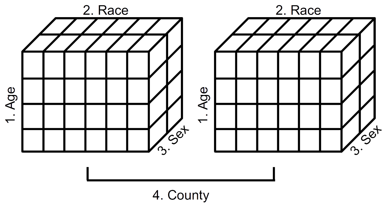
FIGURE 2.1: Schematic representation of a 4-dimensional array (Year 2000 population estimates by age, race, sex, and county)
Displayed in Figure 2.1 is a schematic representation of the 4-dimensional array of population estimates in Table 2.20. The left cube represents the population estimates by age, race, and sex (dimensions 1, 2, and 3) for Alameda County (first component of dimension 4). The right cube represents the population estimates by age, race, and sex (dimensions 1, 2, and 3) for San Francisco County (second component of dimension 4). We see, then, that it is possible to visualize data arrays in more than three dimensions.
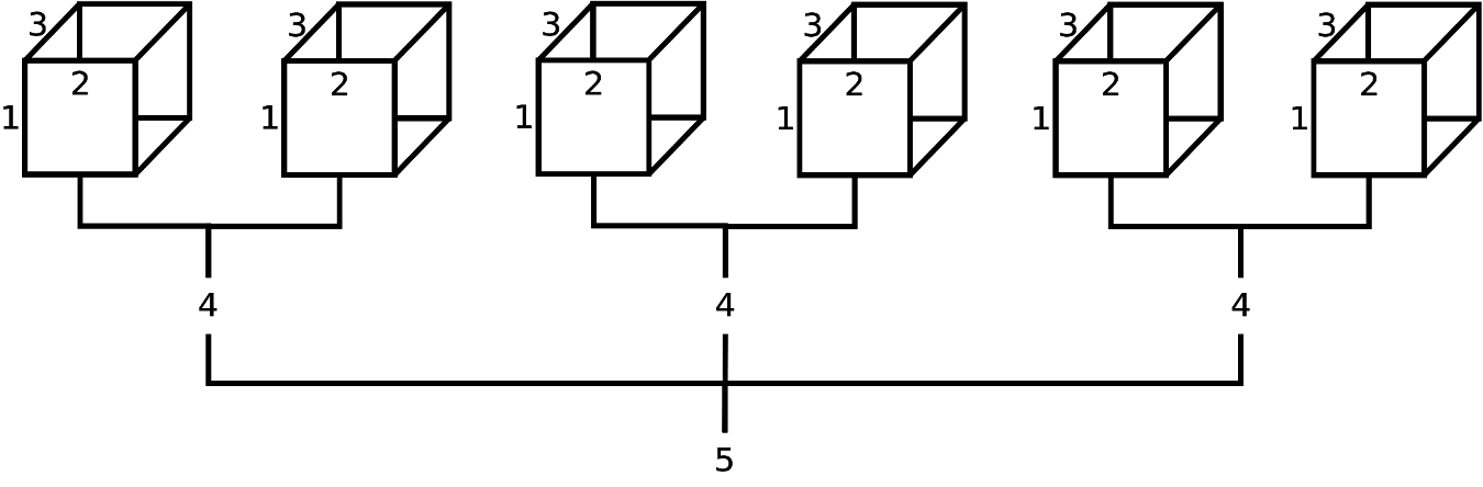
FIGURE 2.2: Schematic representation of a theoretical 5-dimensional array (possibly population estimates by age (1), race (2), sex (3), party affiliation (4), and state (5)). From this diagram, we can infer that the field ‘state’ has 3 levels, and the field ‘party affiliation’ has 2 levels; however, it is not apparent how many age levels, race levels, and sex levels have been created. Although not displayed, age levels would be represented by row names (along 1st dimension), race levels would be represented by column names (along 2nd dimension), and sex levels would be represented by depth names (along 3rd dimension).
To convince ourselves further, displayed in Figure 2.2 is a theorectical 5-dimensional data array. Suppose this 5-D array contained data on age (‘Young’, ‘Old’), ethnicity (‘White’, ‘Nonwhite’), sex (‘Male’, ‘Female’), party affiliation (‘Democrat’, ‘Republican’), and state (‘California’, ‘Washington State’, ‘Florida’). For practice, using fictitious data, try the following R code and study the output:
2.4.2 Creating arrays
In R, arrays are most often produced with the array, table, or
xtabs functions (Table 2.21). As in the
previous example, the array function works much like the matrix
function except the array function can specify 1 or more dimensions,
and the matrix function only works with 2 dimensions.
#> [1] 1#> [,1]
#> [1,] 1#> , , 1
#>
#>      [,1]
#> [1,] 1| Function | Description | Try these examples |
|---|---|---|
array |
Reshapes vector | aa<-array(1:12,dim=c(2,3,2)) |
table |
Cross-tabulate vectors | data(infert) # load infert |
table(infert$educ, infert$spont, infert$case) |
||
xtabs |
Cross-tabulate data frame | xtabs(~education + case + parity, data = infert) |
as.table |
Coercion | ft <- ftable(infert$educ, infert$spont, infert$case) |
as.table(ft) |
||
dim |
Assign dimensions to object | x <- 1:12 |
dim(x) <- c(2, 3, 2) |
The table and xtabs functions cross tabulate two or more
categorical vectors, except that xtabs only works with data frames.
In R, categorical data are represented by character vectors or
factors.18 First, we cross tabulate character vectors
using table and xtabs.
 ## read data 'as is' (no factors created)
udat1 <- read.csv('~/data/ugdp.txt', as.is = TRUE)
str(udat1)
#> 'data.frame': 409 obs. of 3 variables:
#> $ Status : chr "Death" "Death" "Death" "Death" ...
#> $ Treatment: chr "Tolbutamide" "Tolbutamide" "Tolbutamide" "Tolbutamide" ...
#> $ Agegrp : chr "<55" "<55" "<55" "<55" ...#> , , = <55
#>
#>
#> Placebo Tolbutamide
#> Death 5 8
#> Survivor 115 98
#>
#> , , = 55+
#>
#>
#> Placebo Tolbutamide
#> Death 16 22
#> Survivor 69 76The as~is option assured that character vectors
were not converted to factors, which is the default. Notice that the
table function produced an array with no field names (i.e.,
Status, Treatment, Agegrp). This is not ideal. A better option is to
use xtabs, which uses a formula interface (~ V1 + V2):
#> , , Agegrp = <55
#>
#>           Treatment
#> Status     Placebo Tolbutamide
#>   Death          5           8
#>   Survivor     115          98
#>
#> , , Agegrp = 55+
#>
#>           Treatment
#> Status     Placebo Tolbutamide
#>   Death         16          22
#>   Survivor      69          76
Notice that xtabs includes the field names. For
practice with cross tabulating factors, repeat the above expressions
with read in the data setting option as is to FALSE.
Although table does not generate the field names, they can be
added manually:
#> , , Age = <55
#>
#>           Therapy
#> Outcome    Placebo Tolbutamide
#>   Death          5           8
#>   Survivor     115          98
#>
#> , , Age = 55+
#>
#>           Therapy
#> Outcome    Placebo Tolbutamide
#>   Death         16          22
#>   Survivor      69          76
Recall that the ftable function creates a flat contingency
from categorical vectors. The as.table function converts the
flat contingency table back into a multidimensional array.
#>                 Outcome Death Survivor
#> Age Therapy
#> <55 Placebo                 5      115
#>     Tolbutamide             8       98
#> 55+ Placebo                16       69
#> Tolbutamide 22 76#> , , Outcome = Death
#>
#> Therapy
#> Age Placebo Tolbutamide
#> <55 5 8
#> 55+ 16 22
#>
#> , , Outcome = Survivor
#>
#> Therapy
#> Age Placebo Tolbutamide
#> <55 115 98
#> 55+ 69 762.4.3 Naming arrays
Naming components of an array is an extension of naming components of a matrix (Table 2.14). Study and implement the examples in Table 2.22.
| Function | Study and try these examples |
|---|---|
array |
x <- c(140, 11, 280, 56, 207, 9, 275, 32) |
rn <- c('>=1 cups per day', '0 cups per day') |
|
cn <- c('Cases', 'Controls') |
|
dn <- c('Females', 'Males') |
|
x <- array(x, dim = c(2, 2, 2), |
|
dimnames = list(Coffee = rn, |
|
Outcome = cn, Gender = dn)); x |
|
dimnames |
x <- c(140, 11, 280, 56, 207, 9, 275, 32) |
rn <- c('>=1 cups per day', '0 cups per day') |
|
cn <- c('Cases', 'Controls') |
|
dn <- c('Females', 'Males') |
|
x <- array(x, dim = c(2, 2, 2)) |
|
dimnames(x) <- list(Coffee = rn, Outcome = cn, |
|
Gender = dn); x |
|
names |
x <- c(140, 11, 280, 56, 207, 9, 275, 32) |
rn <- c('>=1 cups per day', '0 cups per day') |
|
cn <- c('Cases', 'Controls') |
|
dn <- c('Females', 'Males') |
|
x <- array(x, dim = c(2, 2, 2)) |
|
dimnames(x) <- list(rn, cn, dn) |
|
x # display w/o field names |
|
names(dimnames(x))<-c('Coffee', 'Case status', 'Sex') |
|
x # display w/ field names |
2.4.4 Indexing (subsetting) arrays
Indexing an array is an extension of indexing a matrix (Table 2.15). Study and implement the examples in (Table 2.23).
| Indexing | Try these examples |
|---|---|
| By logical | zz <- x[ ,1,1]>50; zz |
x[zz, , ] |
|
| By position | x[1, , ] |
x[ ,2 , ] |
|
| By name (if exists) | x[ , , 'Males'] |
x[ ,'Controls', 'Females'] |
2.4.5 Replacing array elements
Replacing elements of an array is an extension of replacing elements of a matrix (Table 2.16). Study and implement the examples in (Table 2.24).
| Replacing | Try these examples |
|---|---|
| By logical | x > 200 |
x[x > 200] <- 999 |
|
x |
|
| By position | # use x from Table 2.22 |
x[1, 1, 1] <- NA |
|
x |
|
| By name (if exists) | x[ ,'Controls', 'Females'] <- 99; x |
2.4.6 Operating on an array
With the exception of the aperm function, operating on an array
(Table 2.25) is an extension of operating on a matrix
(Table 2.17). The second group of functions, such as
margin.table, are shortcuts provided for convenience. In other
words, these operations are easily accomplished using apply and/or
sweep.
| Function | Description |
|---|---|
aperm |
Transpose an array by permuting its dimensions |
apply |
Apply a function to the margins of an array |
sweep |
Sweep out a summary statistic from an array |
These short-cuts function use apply and/or sweep |
|
margin.table |
For array, sum of table entries for a given index |
rowSums |
Sum across rows of an array |
colSums |
Sum down columns of an array |
addmargins |
Calculate and display marginal totals of an array |
rowMeans |
Calculate means across rows of an array |
colMeans |
Calculate means down columns of an array |
prop.table |
Generates distribution |
The aperm function is a bit tricky so we illustrated its use.
x <-  c(140, 11, 280, 56, 207, 9, 275, 32)
x <- array(x, dim = c(2, 2, 2))
rn <- c('>=1 cups per day', '0 cups per day') # dim 1 values
cn <- c('Cases', 'Controls')                  # dim 2 values
dn <- c('Females', 'Males')                   # dim 3 values
dimnames(x) <- list(Coffee = rn, Outcome = cn, Gender = dn); x
#> , , Gender = Females
#>
#> Outcome
#> Coffee Cases Controls
#> >=1 cups per day 140 280
#> 0 cups per day 11 56
#>
#> , , Gender = Males
#>
#> Outcome
#> Coffee Cases Controls
#> >=1 cups per day 207 275
#> 0 cups per day 9 32#> , , Coffee = >=1 cups per day
#>
#> Outcome
#> Gender Cases Controls
#> Females 140 280
#> Males 207 275
#>
#> , , Coffee = 0 cups per day
#>
#> Outcome
#> Gender Cases Controls
#> Females 11 56
#> Males 9 32| Age (yrs) | Sex | White | Black | Other | Total |
|---|---|---|---|---|---|
<=19 |
Male | 90 | 1,443 | 217 | 1,750 |
| Female | 267 | 2,422 | 169 | 2,858 | |
| Total | 357 | 3,865 | 386 | 4,608 | |
| 20–29 | Male | 957 | 8,180 | 1,287 | 10,424 |
| Female | 908 | 8,093 | 590 | 9,591 | |
| Total | 1,865 | 16,273 | 1,877 | 20,015 | |
| 30–44 | Male | 1,218 | 8,311 | 1,012 | 10,541 |
| Female | 559 | 4,133 | 316 | 5,008 | |
| Total | 1,777 | 12,444 | 1,328 | 15,549 | |
| 45+ | Male | 539 | 2,442 | 310 | 3,291 |
| Female | 79 | 484 | 55 | 618 | |
| Total | 618 | 2,926 | 365 | 3,909 | |
| Total (by sex & ethnicity) | Male | 2,804 | 20,376 | 2,826 | 26,006 |
| Female | 1,813 | 15,132 | 1,130 | 18,075 | |
| Total (by ethnicity) | 4617 | 35508 | 3956 | 44081 |
Consider the number of primary and secondary syphilis cases in the United State, 1989, stratified by sex, ethnicity, and age (Table 2.26). This table contains the marginal and joint distribution of cases. Let’s read in the original data and reproduce the table results.
#> 'data.frame':    44081 obs. of  3 variables:
#>  $ Sex : Factor w/ 2 levels "Female","Male": 2 2 2 2 2 2 2 2 2 2 ...
#>  $ Race: Factor w/ 3 levels "Black","Other",..: 3 3 3 3 3 3 3 3 3 3 ...
#> $ Age : Factor w/ 4 levels "<=19","20-29",..: 1 1 1 1 1 1 1 1 1 1 ...#> $Sex
#> [1] "Female" "Male"
#>
#> $Race
#> [1] "Black" "Other" "White"
#>
#> $Age
#> [1] "<=19" "20-29" "30-44" "45+"In R, categorical data are converted into factors. The possible
values for each factor are called levels. We used lapply to pass
the levels function and display the levels for each factor. In
order to match the table display we need to reorder the levels for Sex
and Race, and we recode Age into four levels.
sdat5$Sex <- factor(sdat5$Sex, levels = c('Male', 'Female'))
sdat5$Race <- factor(sdat5$Race,levels=c('White','Black','Other'))
lapply(sdat5, levels) # verify
#> $Sex
#> [1] "Male" "Female"
#>
#> $Race
#> [1] "White" "Black" "Other"
#>
#> $Age
#> [1] "<=19" "20-29" "30-44" "45+"We used the factor function and the levels option to reorder the
levels. Now we are ready to create an array and calculate the
marginal totals to replicate Table 2.26.
#> , , Age = <=19
#>
#>         Race
#> Sex      White Black Other
#>   Male      90  1443   217
#>   Female   267  2422   169
#>
#> , , Age = 20-29
#>
#>         Race
#> Sex      White Black Other
#>   Male     957  8180  1287
#>   Female   908  8093   590
#>
#> , , Age = 30-44
#>
#>         Race
#> Sex      White Black Other
#>   Male    1218  8311  1012
#>   Female   559  4133   316
#>
#> , , Age = 45+
#>
#>         Race
#> Sex      White Black Other
#>   Male     539  2442   310
#>   Female    79   484    55
To get marginal totals for one dimension, use the apply function and
specify the dimension for stratifying the results.
#> [1] 44081#> Male Female
#> 26006 18075#> White Black Other
#> 4617 35508 3956#> <=19 20-29 30-44 45+
#> 4608 20015 15549 3909To get the joint marginal totals for 2 or more dimensions, use the
apply function and specify the dimensions for stratifying the
results. This means that the function that is passed to apply is
applied across the other, non-stratified dimensions.
#>         Race
#> Sex      White Black Other
#>   Male    2804 20376  2826
#> Female 1813 15132 1130#> Age
#> Sex <=19 20-29 30-44 45+
#> Male 1750 10424 10541 3291
#> Female 2858 9591 5008 618#> Race
#> Age White Black Other
#> <=19 357 3865 386
#> 20-29 1865 16273 1877
#> 30-44 1777 12444 1328
#> 45+ 618 2926 365In R, arrays are displayed by the 1st and 2nd dimensions, stratified
by the remaining dimensions. To change the order of the dimensions,
and hence the display, use the aperm function. For example,
the syphilis case data is most efficiently displayed when it is
stratified by race, age, and sex:
#> , , Sex = Male
#>
#>        Age
#> Race    <=19 20-29 30-44  45+
#>   White   90   957  1218  539
#>   Black 1443  8180  8311 2442
#>   Other  217  1287  1012  310
#>
#> , , Sex = Female
#>
#>        Age
#> Race    <=19 20-29 30-44  45+
#>   White  267   908   559   79
#>   Black 2422  8093  4133  484
#>   Other  169   590   316   55
Using aperm we moved the 2nd dimension (race) into
the first position, the 3rd dimension (age) into the second position,
and the 1st dimension (sex) into the third position.
Another method for changing the display of an array is to convert it
into a flat contingency table using the ftable function. For
example, to display Table 2.26 as a flat contingency
table in R (but without the marginal totals), we use the following
code:
sdat.asr <- aperm(sdat, c(3,1,2)) # arrange age, sex, race
ftable(sdat.asr)                  # convert 2-D flat table
#> Race White Black Other
#> Age Sex
#> <=19 Male 90 1443 217
#> Female 267 2422 169
#> 20-29 Male 957 8180 1287
#> Female 908 8093 590
#> 30-44 Male 1218 8311 1012
#> Female 559 4133 316
#> 45+ Male 539 2442 310
#> Female 79 484 55This ftable object can be treated as a matrix, but
it cannot be transposed. Also, notice that we can combine the
ftable with addmargins:
#>              Race White Black Other   Sum
#> Age   Sex
#> <=19  Male           90  1443   217  1750
#>       Female        267  2422   169  2858
#>       Sum           357  3865   386  4608
#> 20-29 Male          957  8180  1287 10424
#>       Female        908  8093   590  9591
#>       Sum          1865 16273  1877 20015
#> 30-44 Male         1218  8311  1012 10541
#>       Female        559  4133   316  5008
#>       Sum          1777 12444  1328 15549
#> 45+   Male          539  2442   310  3291
#>       Female         79   484    55   618
#>       Sum           618  2926   365  3909
#> Sum   Male         2804 20376  2826 26006
#>       Female       1813 15132  1130 18075
#>       Sum          4617 35508  3956 44081
To share the U.S. syphilis data in a universal format, we could create
a text file with the data in a tabular form. However, the original,
individual-level data set has over 40,000 observations. Instead, it
would be more convenient to create a group-level, tabular data set
using the as.data.frame function on the data array object.
#> 'data.frame':    24 obs. of  4 variables:
#>  $ Sex : Factor w/ 2 levels "Male","Female": 1 2 1 2 1 2 1 2 1 2 ...
#>  $ Race: Factor w/ 3 levels "White","Black",..: 1 1 2 2 3 3 1 1 2 2 ...
#>  $ Age : Factor w/ 4 levels "<=19","20-29",..: 1 1 1 1 1 1 2 2 2 2 ...
#> $ Freq: int 90 267 1443 2422 217 169 957 908 8180 8093 ...#> Sex Race Age Freq
#> 1 Male White <=19 90
#> 2 Female White <=19 267
#> 3 Male Black <=19 1443
#> 4 Female Black <=19 2422
#> 5 Male Other <=19 217
#> 6 Female Other <=19 169
#> 7 Male White 20-29 957
#> 8 Female White 20-29 908The group-level data frame is practical only if all the fields are categorical data, as is the case here. For additional practice, study and implement the examples in Table 2.25.
2.5 Selected applications
2.5.1 Probabilistic reasoning with Bayesian networks
A Bayesian network (BN) is a graphical model for representing probabilistic, but not necessarily causal, relationships between variables called nodes [11,12]. The nodes are connected by lines called edges which, for our purposes, are always directed with an arrow. Consider this noncausal BN:
Smelling smoke increases the probability of a fire burning nearby, but obviously smoke alone does not cause a fire. In other words, does knowing \(X\) (smell smoke) change the credibility of \(Y\) (fire nearby)? In contrast, now consider this causal BN:
This causal BN depicts fire causing smoke. Notice that both noncausal and causal BNs have probabilistic dependence which we will use for probabilistic reasoning. Noncausal BNs are commonly used in influence diagrams for decision analysis which we cover later in the book.
A two-node causal BN has two types of proabilistic reasoning (Table ).
| Probabilistic reasoning | Conditional probability |
|---|---|
| Causal (predictive) reasoning | \(P(\text{Effect}\mid\text{Cause})\) |
| Evidential (diagnostic) reasoning | \(P(\text{Cause}\mid\text{Effect})\) |
When a causal effect is not firmly established, the BN asserts this concept:
| Conditional probabilities | Probabilistic reasoning |
|---|---|
| \(P(\text{Evidence}\mid\text{Hypothesis})\) | Causal reasoning |
| \(P(\text{Hypothesis}\mid\text{Evidence})\) | Evidential reasoning |
Evidential reasoning requires Bayes Theorem.
\[ P(H \mid E) = \frac{P(E \mid H)P(H)}{P(E)} \]
\(P(H)\) is the prior (old) belief, \(P(H \mid E)\) is the posterior (new) belief, and \(P(E \mid H)\) is called the likelihood. The likelihood is critical because it is usually measurable. The challenge is that we need Bayes Theorem for two reasons:
- to use evidence and theory to update our belief from \(P(H)\) to \(P(H \mid E)\), and
- to avoid the fallacy of the transposed conditional; i.e., confusing \(P(E \mid H)\) with \(P(H \mid E)\).
2.5.1.1 Example: HIV testing
For example, from Neapolitan (p. 491, [13]), suppose Sam takes a test (evidence) to determine whether he has HIV infection (hypothesis). Here is the BN:
In diagnostic testing we use Bayes Theorem to calculate the post-test probability from the test results, pre-test probability (prevalence of infection), and test characteristics (sensitivity, specificity). Table displays the data we need for applying Bayes Theorem.
| Name | Probabilities | Value |
|---|---|---|
| Pre-test (prior) probability of \(\text{HIV}+\) | \(P(\text{HIV}+)\) | 0.00001 |
| Sensitivity | \(P(\text{Test}+\mid\text{HIV}+)\) | 0.999 |
| Specificity | \(P(\text{Test}-\mid\text{HIV}-)\) | 0.998 |
| Post-test (posterior) probability | \(P(\text{HIV}\mid\text{Test})\) | TBD |
For illustrative purposes, we calculate the “positive predictive value” (PPV).
\[ P(H+ \mid T+) = \frac{P(T+ \mid H+)P(H+)}{P(T+ \mid H+)P(H+) + P(T+ \mid H-)P(H-)} \]
This is easy to calculate in R.
#> [1] 0.004970223Calculating the PPV (or NPV) is evidential reasoning and it requires applying Bayes Theorem. Our brains are not capable of this calculation; we need computational tools. In other words, our brains are not able to “flip the arrow” from \(P(\text{Evidence}\mid{Hypothesis})\) to \(P(\text{Hypothesis}\mid \text{Evidence})\) and make valid Bayesian calculations.
2.5.2 Causal graphs—the story behind the data
2.5.2.1 Example: A retrospective observation study
A vector is represented by a single node. A matrix is represented by two nodes. A 3-dimensional array is represented by three nodes. And, an n-dimensional array is represented by n nodes. For now, these arrays are stratified contigency tables. The story is how the data was generated (data generating process) and how the data was measured (study design). With a causal graph we encode the salient parts of the story.
In 1986, Charig published a retrospective observational study comparing open surgery (Treatment A) to percutaneous nephrolithotomy (Treatment B) for the treatment of kidney stones [14,15]. Treatment B is noninvasive. Success was defined as no stones at three months. The data are presented in Table 2.27.
| Stone size | Treatment A | Success (%) | Treatment B | Success (%) | |
|---|---|---|---|---|---|
| Small stones | 81/87 | 93 | 234/270 | 87 | |
| Large stones | 192/263 | 73 | 55/80 | 69 | |
| Combined | 273/350 | 78 | 289/350 | 83 |
If you believe in “data-driven” decision-making then you have a big problem! When you stratify the data by stone size, Treatment A is better. However, when you do not stratify by stone size, Treatment B is better. Which is correct? No amount of data analysis will answer this question—that’s why it’s call a paradox—in this case, Simpson’s paradox. We need more information (the story) and we need a method (causal graph) to encode this story.
We have three variables: \(X\): treatment (A, B), \(Y\): success (yes, no), \(Z\): stone size (small, large). How are they related? The obvious relationship is the causal effect of Treatment on Success.
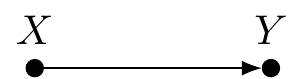
FIGURE 2.3: Causal graph of treatment (X) and success (Y)
dat1 <- c(273, 350-273, 289, 350-289)
dat1 <- array(dat1, dim = c(2, 2), dimnames = list("Success (Y)"
                 = c('Yes', 'No'), "Treatment (X)" = c('A', 'B')))
dat1
#> Treatment (X)
#> Success (Y) A B
#> Yes 273 289
#> No 77 61#> Treatment (X)
#> Success (Y) A B
#> Yes 0.78 0.8257143
#> No 0.22 0.1742857Now, here is the missing story: It turns out that urologists select open surgery (Treatment A) for more severe cases, and larger stones are considered more severe. In other words, severity causes a selection bias, and we can see the resulting association in the data.
dat2 <- c(87, 270, 263, 80)
dat2 <- array(dat2, dim = c(2,2), dimnames = list("Treatment (X)"
          = c('A', 'B'), "Stone.Size (Z)" = c('Small', 'Large')))
dat2
#> Stone.Size (Z)
#> Treatment (X) Small Large
#> A 87 263
#> B 270 80#> Stone.Size (Z)
#> Treatment (X) Small Large
#> A 0.2436975 0.7667638
#> B 0.7563025 0.2332362Of course, stone size (i.e., severity) has a causal effect on success. We now have enough information to construct the full causal graph (Figure 2.4).
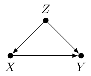
FIGURE 2.4: Causal graph of treatment (X), success (Y), and stone size (Z).
Figure 2.4 depicts the three possible patterns we can observe with three nodes:
- chain (sequential cause): \(Z \rightarrow X \rightarrow Y\)
- fork (common cause): \(X \leftarrow Z \rightarrow Y\)
- collider (common effect): \(X \rightarrow Y \leftarrow Z\)
In this causal graph (Figure 2.4), the stone size (\(Z\)) is a common cause (fork) and is also called a confounder because it distorts the causal effect of treatment (\(X\)) on success (\(Y\)).
Later we will learn how to use the causal graph to derive an adjustment formula to de-confound the causal effect of treatment on success. This is not possible with the data table alone; the causal graph encodes the story, allowing us to adjust for confounding.
KEY IDEA: All causal graphs, regardless of complexity, are constructed from the three core patterns: chain (sequential cause), fork (common cause), and collider (common effect). The causal graph encodes the “story” of the data generating process. By itself the data tables never tell the full story—we need a causal graph.
2.5.2.2 Conditional probability tables in R
A directed acyclic graph (DAG) is a causal Bayesian network (BN). A BN is a probabilistic graphical model where nodes are conditional probability tables and connecting arrows encode probabilistic dependence. Depending on the probabilistic assessment, in BNs arrows can “flip.” However, in DAGs the arrows cannot flip because they represent causal effects, yet we can still evaluate a DAG as a probabilistic graphical model.
For example, Figure 2.4 represents data that has a joint probability distribution. Using product decomposition we can rewrite it as a product of conditional probabilities that we read directly from the DAG.
\[ \Pr(X,Y,Z) = \Pr(Z) \Pr(X \mid Z) \Pr(Y \mid X, Z) \]
There are no arrows into node \(Z\) so this is represented by the marginal probability \(\Pr(Z)\). There is an arrow from parent node \(Z\) to child node \(X\); therefore, we have the conditional probability \(\Pr(X \mid Z)\). Finally, we have an arrow from \(X\) to \(Y\) and from \(Z\) to \(Y\); therefore, we have the conditional probability \(\Pr(Y \mid X, Z)\).
Using the data from Table 2.27, let’s use R to construct these conditional probability tables. We start with \(\Pr(Y \mid X, Z)\).
dat.yxz <- c(81, 87-81, 234, 270-234, 192, 263-192, 55, 80-55)
dat.yxz <- array(dat.yxz, dim = c(2,2,2), dimnames
   = list("Success (Y)"=c('Yes','No'), "Treatment (X)"=c('A','B'),
                           "Stone.size (Z)" = c('Small','Large')))
dat.yxz
#> , , Stone.size (Z) = Small
#>
#> Treatment (X)
#> Success (Y) A B
#> Yes 81 234
#> No 6 36
#>
#> , , Stone.size (Z) = Large
#>
#> Treatment (X)
#> Success (Y) A B
#> Yes 192 55
#> No 71 25#> , , Stone.size (Z) = Small
#>
#> Treatment (X)
#> Success (Y) A B
#> Yes 0.93103448 0.8666667
#> No 0.06896552 0.1333333
#>
#> , , Stone.size (Z) = Large
#>
#> Treatment (X)
#> Success (Y) A B
#> Yes 0.730038 0.6875
#> No 0.269962 0.3125Notice what the option margin = c(2, 3) accomplished: “Stratified by
dimensions 2 (\(X\)) and 3 (\(Z\)), provide the distribution along the
remaining dimension(s) (in this case, dimension 1 or \(Y\)).” This
enables us to assess the probability of success given treatment,
stratified by stone size (severity).
Now, let’s construct \(\Pr(X \mid Z)\). Recall, we already
constructed this two-way table de novo, but now we use the apply
function instead.
#>              Stone.size (Z)
#> Treatment (X) Small Large
#>             A    87   263
#> B 270 80#> Stone.size (Z)
#> Treatment (X) Small Large
#> A 0.2436975 0.7667638
#> B 0.7563025 0.2332362This table is the crude, combined or unstratified table.
Finally, let’s construct \(\Pr(Z)\), again using apply.
#> Small Large
#> 357 343#> Small Large
#> 0.51 0.49Consider DAGs (Figure 2.4) and data (Table 2.27) two sides of the same coin. They both give us different but complementary information. Causal models represent our beliefs or hypotheses of how the world works (the story). As the world unfolds it generates data which we can measure and analyze. Because one particular instance of data (e.g., a stratified contingency table) can be generated from many different data generating processes we need a causal model to guide us. For now, we are learning to use R to encode this information (data) and knowledge (DAG).
2.6 Exercises
File \(\rightarrow\) New Project
\(\rightarrow\) New Directory \(\rightarrow\) Empty Project. Name the
new directory ph251d-hwk. At the R console, use R to display
the file path to the work directory containing .RData?
Exercise 2.2 (Recreate 2 x 2 Table) The Whickham data set is “Data on age, smoking, and mortality from a
one-in-six survey of the electoral roll in Whickham, a mixed urban and
rural district near Newcastle upon Tyne, in the UK. The survey was
conducted in 1972–1974 to study heart disease and thyroid disease. A
follow-up on those in the survey was conducted twenty years later.
This dataset contains a subset of the survey sample: women who were
classified as current smokers or as never having smoked.” (source:
mosaicData package)
A data frame with 1314 observations on women for the following variables:
outcome: survival status after 20 years: a factor with levels Alive Deadsmoker: smoking status at baseline: a factor with levels No Yesage: age (in years) at the time of the first survey
matrix, cbind, rbind, dimnames, or names functions.
| Outcome | Smoker | |
|---|---|---|
| Yes | No | |
| Dead | 139 | 230 |
| Alive | 443 | 502 |
apply, cbind, rbind, names, and dimnames functions, recreate the Table 2.29.
| Outcome | Smoker | ||
|---|---|---|---|
| Yes | No | Total | |
| Dead | 139 | 230 | 329 |
| Alive | 443 | 502 | 945 |
| Total | 582 | 732 | 1314 |
sweep and apply functions to calculate row, column, and joint
probability distributions (i.e., create three tables with proportions).
| Measure | Smoker | |
|---|---|---|
| Yes | No | |
| Risk | 0.24 | 0.31 |
| Risk Ratio | 0.76 | 1.00 |
| Odds | 0.31 | 0.46 |
| Odds Ratio | 0.68 | 1.00 |
mosaicData R package. Load the Whickham data
set. Using the xtabs function create two-way and three-way
contingency tables. Calculate “measures of associations.” What is
your interpretation? Here is some R code to get you started.
## install.packages("mosaicData")
library(mosaicData)
data(Whickham)
wdat <- Whickham
## discretize age into 4-level categorical variable
wdat$age4 <- cut(wdat$age, breaks=c(15, 25, 45, 65, 100),
right = FALSE)tapply function to calculate the mean age at study entry comparing
(a) smokers to non-smokers,
(b) dead vs. alive,
(c) smoker status stratified by outcome status (2 x 2 table).
References
8. Olsen SJ, Chang H-L, Cheung TY-Y, Tang AF-Y, Fisk TL, Ooi SP-L, et al. Transmission of the severe acute respiratory syndrome on aircraft. N Engl J Med. 2003 Dec;349(25):2416–22.
9. The GenIUSS Group. Best practices for asking questions to identify transgender and other gender minority respondents on population-based surveys [Internet]. The Williams Institute; 2014. Available from: https://williamsinstitute.law.ucla.edu/wp-content/uploads/geniuss-report-sep-2014.pdf
10. Rothman K. Epidemiology: An introduction. 2nd ed. New York, NY: Oxford University Press; 2012.
11. Scutari M, Denis J-B. Bayesian networks: With examples in r. Boca Raton: Chapman; Hall; 2014.
12. Fenton N, Neil M. Risk assessment and decision analysis with bayesian networks. Chapman; Hall/CRC; 2 edition; 2019.
13. Neapolitan R, Jiang X, Ladner DP, Kaplan B. A primer on Bayesian decision analysis with an application to a kidney transplant decision. Transplantation. 2016 Mar;100(3):489–96.
14. Charig CR, Webb DR, Payne SR, Wickham JE. Comparison of treatment of renal calculi by open surgery, percutaneous nephrolithotomy, and extracorporeal shockwave lithotripsy. Br Med J (Clin Res Ed). 1986 Mar;292(6524):879–82.
15. Julious SA, Mullee MA. Confounding and simpson’s paradox. BMJ. 1994 Dec;309(6967):1480–1.
In other programming languages, vectors are either row vectors or column vectors. R does not make this distinction until it is necessary. Do not confuse a vector, as discussed in this section, with the
vectorfunction which can create atomic or recursive objects.↩In other programming languages, vectors are either row vectors or column vectors. R does not make this distinction until it is necessary. Do not confuse a vector, as discussed in this section, with the
vectorfunction which can create atomic or recursive objects.↩See also the
curvefunction for graphing mathematical equations.↩More specifically,
rowSums,colSums,rowMeans, andcolMeansare optimized for speed.↩For now, consider factors as character vectors where the possible values (called levels) have been specified. We cover factors later.↩