Chapter 1 Getting Started With R
1.1 What is R?
R is a freely available “computational language and environment for data analysis and graphics.” R is indispensable for anyone that uses and interprets data. As medical, public health, and research epidemiologists, we use R in the following ways:
- Full-function calculator
- Extensible statistical package
- High-quality graphics tool
- Multi-use programming language
We use R to explore, analyze, and understand public health data. We analyze data straight out of tables provided in reports or articles as well as analyze usual data sets. The data might be a large, individual-level data set imported from another source (e.g., cancer registry); an imported matrix of group-level data (e.g, population estimates or projections); or some data extracted from a journal article we are reviewing. The ability to quantitatively express, graphically explore, and describe data and processes enables one to work and strengthen one’s epidemiologic intuition.
In fact, we only use a very small fraction of the R package. For those who develop an interest or have a need, R also has many of the statistical modeling tools used by epidemiologists and statisticians, including logistic and Poisson regression, and Cox proportional hazard models. However, for many of these routine statistical models, almost any package will suffice (SAS, Stata, SPSS, etc.). The real advantage of R is the ability to easily manipulate, explore, and graphically display data. Repetitive analytic tasks can be automated or streamlined with the creation of simple functions (programs that execute specific tasks). The initial learning curve is steep, but in the long run one is able to conduct analyses that would otherwise require a tremendous amounts of programming and time.
Some may find R challenging to learn if they are not familiar with statistical programming. R was created by statistical programmers and is more often used by analysts comfortable with matrix algebra and programming. However, even for those unfamiliar with matrix algebra, there are many analyses one can accomplish in R without using any advanced mathematics, which would be difficult in other programs. The ability to easily manipulate data in R will allow one to conduct good descriptive epidemiology, life table methods, graphical displays, and exploration of epidemiologic concepts. R allows one to work with data in any way they come.
1.2 What is RStudio?
To get started quickly we need tools that makes the process of writing and compiling R code quick and (mostly) pain free. Fortunately for us there is RStudio6—it is a free, open source, and powerful integrated development environment (IDE) for R that runs on most operating systems (Windows, Mac, or Linux). After installing R, install RStudio—it has all the tools we need to learn and apply R.
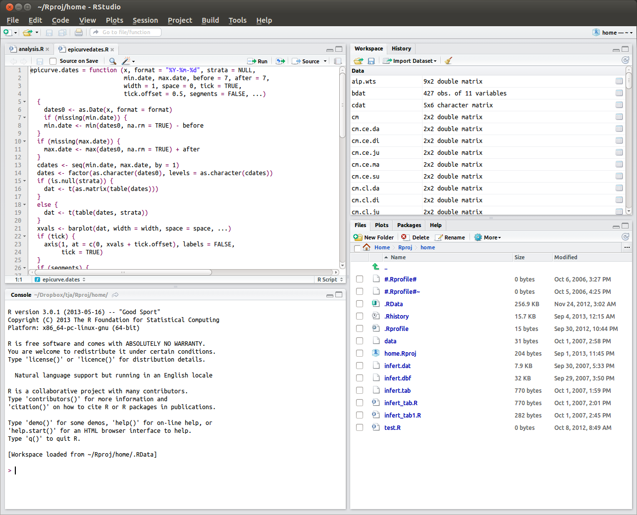
FIGURE 1.1: Screenshot of RStudio in Ubuntu Linux: Top left is for R script editor, or for viewing tabular data objects. Top right has tabs for workspace and history. Bottom right has tabs for files, plots, packages, or help. Bottom left is the console for typing R expressions for evaluation.
1.3 Who should learn R?
Anyone that uses a calculator or spreadsheet, or analyzes numerical data at least weekly should seriously consider learning and using R. This includes data scientists, epidemiologists, statisticians, physician researchers, engineers, health economists, health systems analysts, business analysts, and faculty and students of mathematics and science courses, to name just a few. We jokingly tell our staff analysts that once they learn R they will never use a spreadsheet program again (well almost never!).
1.4 Why should I learn R?
To implement numerical methods we need a computational tool. On one end of the spectrum are calculators and spreadsheets for simple calculations, and on the other end of the spectrum are specialized computer programs for such things as statistical and mathematical modeling. However, many numerical problems are not easily handled by these approaches. Calculators, and even spreadsheets, are too inefficient and cumbersome for numerical calculations whose scope and scale change frequently. Statistical packages are usually tailored for the statistical analysis of data sets and often lack an intuitive, extensible, open source programming language for tackling new problems efficiently. R can do the simplest and the most complex analysis efficiently and effectively.
When we learn and use R regularly we will save significant amounts of time and money. It’s powerful and it’s free! It’s a complete environment for data analysis and graphics. Its straightforward programming language facilitates the development of functions to extend and improve the efficiency of our analyses.
1.5 Where can I get R?
R is available for many computer platforms, including Linux, Mac OS, Microsoft (MS) Windows, and others. R comes as source code or a binary file. Source code needs to be compiled into an executable program for your computer. Those not familiar with compiling source code (and that’s most of us) just install the binary program. We assume most readers will be using R in the Mac OS or MS Windows environment. Listed here are useful R links:
- R Project home page at http://www.r-project.org
- R download page at http://cran.r-project.org
- Numerous free tutorials are at http://cran.r-project.org/other-docs.html
- R Wikibook at http://en.wikibooks.org/wiki/R_Programming
- R Journal at http://journal.r-project.org
To install R for Windows or Mac OS, do the the following:
- Go to http://www.r-project.org;
- From the left menu list, click on the “CRAN” (Comprehensive R Archive Network) link;
- Select a nearby geographic site (e.g., http://cran.cnr.berkeley.edu);
- Select appropriate operating system;
- Select on “base” link;
- For Windows, save
R-3.6.X-win.exeto the computer; and for Mac OS, save theR-3.6.X.pkginstaller package. For Linux, install from the Debian repository, or follow instruction on the CRAN site. - Run the installation program and accept the default installation options.
- Install RStudio (https://www.rstudio.com/). That’s it!
An alternative to installing R on a computer is using RStudio Cloud. From a web browser one runs R as if it were on their computer. This resolves occasional quirks of installing and updating R, RStudio, and R packages on a personal computer.
1.6 How do I use R?
1.6.1 Using R on our computer
Use R by typing commands at the R console (>) and pressing Enter on
our keyboard. This is how to use R interactively. Alternatively,
from the R console, we can also execute a list of R commands that we
have saved in a text file (more on this later). Here is an example of
using R as a calculator:
#> [1] 750Use the c function to collect data entered at the console.
Name each collection of data, and then perform a numercal operation.
In this example we conduct an analysis that is analogous to working in
a spreadsheet.
quantity <- c(34, 56, 22)        # quantity data
price <- c(19.95, 14.95, 10.99)  # price data
subtotal <- quantity*price       # subtotal cost
cbind(quantity, price, subtotal) # column bind, like spreadsheet
#> quantity price subtotal
#> [1,] 34 19.95 678.30
#> [2,] 56 14.95 837.20
#> [3,] 22 10.99 241.781.6.2 Does R have epidemiology programs?
The default installation of R does not have packages that specifically implement epidemiologic applications; however, many of the statistical tools that epidemiologists use are readily available, including statistical models such as unconditional logistic regression, conditional logistic regression, Poisson regression, Cox proportional hazards regression, and much more. R now has a impressive collection of packages with methods applied to epidemiologic problems. To see more visit https://cran.r-project.org/web/packages/ and search on “epi.” The focus of this book is learning how to use R without relying on too heavily on specific packages. Learning the R basics covered in this book will help one take full advantage of these and other R packages, some of which address advanced topics such as network modeling of epidemics.
1.6.3 How should I use these notes?
The best way to learn R is to use it! Use it as your calculator! Use
it as your spreadsheet! Finally read these notes sitting at a
computer and use R interactively (this works best sitting in a cafe
that brews great coffee and plays good music). Although we initially
encourage you to use R interactively by typing expressions at the
console, as a general rule, it is much better to type your code as a R
script. Save your code with a convenient file name such as
job01.R.7
RStudio comes with a text editor for creating and editing R scripts. Our focus will be learning how to use RStudio to edit and run R scripts.
The code in your text editor can be run in the following ways:
- highlight and run selected expressions in the RStudio,
- copy and paste the code directly into R console, or
- run the file in batch mode from the R console using the
sourcefunction (e.g.,source("job01.R")).
| Expression type | Operator | Example | Value |
|---|---|---|---|
| addition | + |
5+4 |
9 |
| subtraction | - |
5-4 |
1 |
| multiplication | * |
5*4 |
20 |
| division | / |
10/3 |
3.333333 |
| integer divide | %/% |
10%/%3 |
3 |
| modulus (remainder) | %% |
10%%3 |
1 |
| unary minus | - |
-(-5) |
5 |
| absolute value | abs |
abs(-23) |
23 |
| exponentiation8 | ^ |
5^4 |
625 |
| exponentiation (base \(e\)) | exp |
exp(8) |
2980.958 |
| logarithm | log |
log(exp(8)) |
8 |
| square root | sqrt |
sqrt(64) |
8 |
1.7 Just do it!
1.7.1 Using R as your calculator
Open R and start using it as our calculator. The most common math operators are displayed in Table 1.1. From now on make R your default calculator! Study the examples and spend a few minutes experimenting with R as a calculator. Use parentheses as needed to group operations. Use the keyboard Up-arrow to recall what we previously entered at the command line prompt.
1.7.2 Useful R concepts
1.7.2.1 Types of evaluable expressions
Every expression that is entered at the R console is evaluated by
R and returns a value. A literal expression is the simplist
expression that can be evaluated (number, character string, or logical
value). Mathematical operations involve numeric literals. For
example, R evaluates the expression 4*4 and returns the value 16.
The exception to this is when an evaluable expression is assigned an
object name: x <- 4*4. To display the assigned expression, wrap the
expression in parentheses: (x <- 4*4), or type the object
name. Finally, evaluable expressions must be separated by either
newline breaks or a semicolon. Table 1.2 summarizes
evaluable R expressions.
#> [1] 16#> [1] 16#> [1] 16#> [1] 16| Expression type | Example | Value returned |
|---|---|---|
| literal | 'hello' # character |
"hello" |
3.5 # numeric |
3.5 |
|
TRUE # logical |
TRUE |
|
| math operation | 6*7 |
42 |
| assignment | x <- 4*4 |
none |
x = 4*4 |
none | |
| data object | x |
16 |
| function | sqrt(x) |
4 |
1.7.2.2 Using the assignment operator
Most calculators have a memory function: the ability to assign a
number or numerical result to a key for recalling that number or
result at a later time. The same is true in R but it is much more
flexible. Any evaluable expression can be assigned a name and
recalled at a later time. We refer to these variables as data
objects. We use the assignment operator (<-) to name an
evaluable expression and save it as a data object.
#> [1] "hello, what's your name"Multiple assignments work and are read from right to left:
#> [1] 5#> [1] 5Data objects can be used in subsequent calculations:
#> [1] 25However, updating an object on right side of the assignment does not automatically update the value of the object on the left side of the assignment. To update the left side we must re-run the assignment expression.
#> [1] 25#> [1] 125Finally, similar to Python, the equal sign (=) can be used for
assignment, although we prefer and the <- symbol.
The reason we prefer <- for assigning object names in the
workspace is because later we use = for assigning values to
function arguments. For example,
The first x is an object name assignment in the workspace which
persist during the R session. The second x is a function argument
assignment which is only recognized locally in the function and only
for the duration of the function execution. For clarity, it is better
to keep these types of assignments separate in our mind by using
different assignment symbols.
Study these previous examples and spend a few minutes using the
assignment operator to create and call data objects. Try to use
descriptive names if possible. For example, suppose we have data on
age categories; we might name the data agecat,
age.cat, or age_cat.9
1.7.3 Useful R functions
When we start R we have opened a workspace. The first time
we use R, the workspace is empty. Every time we create a data
object, it is in the workspace. If a data object with the same name
already exists, the old data object will be overwritten without
warning, so be careful! To list the objects in your workspace use the
ls or objects functions:
#> [1] "aa" "ages" "bb" "cc"Data objects can be saved between sessions. We will be prompted with
“Save workspace image?” You can also use save.image() at the
console prompt. The workspace image is saved in a file called
.RData.10 Use getwd() to display the file path to the
.RData file. Table 1.3 has more useful R
functions.
| Function example | Description |
|---|---|
q() |
Quit R |
ls() |
List objects |
rm(object name) |
Remove object |
rm(list = ls()); ls() |
Removes all objects—caution! |
help() |
Open help instructions; |
help(function.name) |
or get help on specific function |
?function.name |
Equivalent to get help |
help.search("print") |
Search help system |
help.start() |
Start help browser |
apropos("plot") |
Displays all objects matching topic |
getwd() |
Working directory (location of .RData) |
setwd("c:\mywork\rproj") |
Set working directory |
args(sample) |
Display arguments of function |
example(plot) |
Runs example of a function |
data() #displays |
Information on available R data sets |
data(data.set.name) |
Load data set |
save.image() |
Saves current workspace to .RData |
1.7.3.1 What are packages?
R has many available functions, and a package is a compiled
collection of functions with a shared purpose or common theme. When
we open R, several packages are attached by default. Each package has its own suite of functions.
To display the list of attached packages use the search function.
To display the file paths to the packages use the searchpaths
function.
#>  [1] ".GlobalEnv"         "package:foreign"
#>  [3] "package:survival"   "package:mosaicData"
#>  [5] "ESSR"               "package:stats"
#>  [7] "package:graphics"   "package:grDevices"
#>  [9] "package:utils"      "package:datasets"
#> [11] "package:methods"    "Autoloads"
#> [13] "package:base"To install a package we enter install.packages(""). For example to install and load the package for
survival analysis we enter
To learn more about a specific package enter library(help=). Alternatively, we can get more detailed information by
entering help.start() which opens the HTML help page. On this page
click on the Packages link to see the available packages. If we need
to load a package enter library(). For example,
when we cover survival analysis we will need to load the survival
package.
1.7.3.2 What are function arguments?
We will be using many R functions for data analysis, so we need to
know some function basics. Suppose we are interested in taking a
random sample of days from the month of June, which has 30 days. We
want to use the sample function but we forgot the syntax.
Let’s explore:
#> function (x, size, replace = FALSE, prob = NULL)
#> {
#>     if (length(x) == 1L && is.numeric(x) && is.finite(x) && x >=
#>         1) {
#>         if (missing(size))
#>             size <- x
#>         sample.int(x, size, replace, prob)
#>     }
#>     else {
#>         if (missing(size))
#>             size <- length(x)
#>         x[sample.int(length(x), size, replace, prob)]
#>     }
#> }
#> <bytecode: 0x7ff828047968>
#> <environment: namespace:base>
Whoa! What happened? Whenever we type the function name
without any parentheses it usually returns the whole function code.
This is useful when we start programming and we need to alter an
existing function, borrow code for our own functions, or study the
code for learning how to program. If we are already familiar with the
sample function we may only need to see the syntax of the
function arguments. For this we use the args function:
#> function (x, size, replace = FALSE, prob = NULL)
#> NULL
The terms x, size, replace, and prob are the function
arguments. First, notice that replace and prob have default
values; that is, we do not need to specify these arguments unless we
want to override the default values. Second, notice the order of the
arguments. If you enter the argument values in the same order as the
argument list we do not need to specify the argument.
#> [1] 18 5 30 23 3 6 13 12 27 19 1 8 25 22 21 28Third, if we enter the arguments out of order then we will get either an error message or an undesired result. Arguments entered out of their default order need to be specified.
#> [1] 15#> [1] 4 18 14 6 11 10 3 12 25 22 9 27 28 5 26 19Fourth, when we specify an argument we only need to type a sufficient number of letters so that R can uniquely identify it from the other arguments.
#> [1] 12 23 22 16 12 17 13 15 5 19 25 7 3 9 27 23Fifth, argument values can be any valid R expression
(including functions) that evaluates to an appropriate value. In the
following example we see two sample functions that provide random
values to the sample function arguments.
#> [1] 8Finally, if we need more guidance on how to use the
sample function enter ?sample or help(sample).
1.7.4 How do I get help?
RStudio has extensive help capabilities. From the RStudio main menu
select Help \(\rightarrow\) R Help to get you started.
The Frequently Asked Questions (FAQ) and R manuals are available from
this menu. From the R console, try the following options to learn
about the help capabilities:
?help               # opens help page for 'help' function
help.start()        # launches HTML help page
help.search("help") # searches help system for "help"
apropos("help")     # displays 'help' objects in search list
To learn about about available data sets use the
data function:
1.7.5 Is there anything else that I need?
Not really. RStudio has everything you will need to use R productively. Some analysts will select to use R with a text editor, rather than RStudio. Like RStudio, a good text editor makes programming and data processing easier and more efficient. If you are considering a text editor, the functionality we look for in a text editor are the following:
- Toggle between wrapped and unwrapped text
- Block cutting and pasting (also called column editing)
- Easy macro programming
- Search and replace using regular expressions
- Ability to import small data sets for editing
When we are programming we want our text to wrap so we can read all of your code. When we import a data set that is wider than the screen, we do not want the data set to wrap: we want it to appear in its tabular format. Column editing allows us to cut and paste columns of text at will. A macro is just a way for the text editor to learn a set of keystrokes (including search and replace) that can be executed as needed. Searching using regular expressions means searching for text based on relative attributes. For example, suppose you want to find all words that begin with “b”, end with “g”, have any number of letters in between but not “r” and “f”. Regular expression searching makes this a trivial task. These are powerful features that once we use regularly, we will wonder how we ever got along without them.
If we do not want to install a text editing program then we can use the default text editor that comes with our computer operating system (gedit in Ubuntu Linux, TextEdit in Mac OS, Notepad in Windows). However, it is much better to install a text editor that works with R. My favorite text editor is the free and open source GNU Emacs.11 GNU Emacs can be extended with the “Emacs Speaks Statistics” (ESS) package. For more information on Emacs and ESS pre-installed for Windows or Mac OS, visit http://ess.r-project.org.
1.7.6 What’s ahead?
To the novice user, R may seem complicated and difficult to learn. In fact, for its immense power and versatility, R is easier to learn and deploy compared to other statistical software (e.g. SAS, Stata, SPSS). This is because R was built from the ground up to be an efficient and intuitive programming environment and language. If you understand the logic and structure of R, then learning proceeds quickly. Just like a spoken language, once you know its rules of grammar, syntax, and pronunciation, and can write legible sentences, you can figure out how to communicate almost anything. Before we get into the “trees” (next chapter), we want to describe the “forest”: the logic and structure of working with R objects and epidemiologic data.
1.7.6.1 Working with R objects
For our purposes, there are only five types of data objects in R12 and five types of actions we take on these objects (Table 1.4). That’s it! No more, no less. You will learn to create, name, index (subset), replace components of, and operate on these data objects using a systematic, comprehensive approach. As you learn about each new data object type, it will reinforce and extend what you learned previously.
| Action | Vector | Matrix | Array | List | Data frame |
|---|---|---|---|---|---|
| Creating | 2.6 | 2.13 | 2.21 | 3.1 | 3.7 |
| Naming | 2.7 | 2.14 | 2.22 | 3.2 | 3.8 |
| Indexing | 2.8 | 2.15 | 2.23 | 3.3 | 3.9 |
| Replacing | 2.9 | 2.16 | 2.24 | 3.4 | 3.10 |
| Operating on | 2.10, 2.11 | 2.17 | 2.25 | 3.5 | 3.11 |
A vector13 is a collection of elements (often numbers):
#> [1] 1 2 3 4 5 6 7 8 9 10 11 12A matrix is a 2-dimensional representaton of a vector:
#>      [,1] [,2] [,3] [,4] [,5] [,6]
#> [1,]    1    3    5    7    9   11
#> [2,]    2    4    6    8   10   12
An array is an \(n\) dimensional represention of a vector:
#> , , 1
#>
#>      [,1] [,2] [,3] [,4] [,5] [,6]
#> [1,]    1    2    3    4    5    6
#>
#> , , 2
#>
#>      [,1] [,2] [,3] [,4] [,5] [,6]
#> [1,]    7    8    9   10   11   12
A list is a collection of “bins”, each containing any kind of R object:
#> [[1]]
#>  [1]  1  2  3  4  5  6  7  8  9 10 11 12
#>
#> [[2]]
#>      [,1] [,2] [,3] [,4] [,5] [,6]
#> [1,]    1    3    5    7    9   11
#> [2,]    2    4    6    8   10   12
#>
#> [[3]]
#> , , 1
#>
#>      [,1] [,2] [,3] [,4] [,5] [,6]
#> [1,]    1    2    3    4    5    6
#>
#> , , 2
#>
#>      [,1] [,2] [,3] [,4] [,5] [,6]
#> [1,]    7    8    9   10   11   12
A data frame is a list in tabular form where each “bin” contains a data vector of the same length. A data frame is the usual tabular data set familiar to epidemiologists. Each row is an record and each column (“bin”) is a field.
smoker <- c("Y", "Y", "N", "N", "Y", "Y", "Y", "N", "Y")
cancer <- c("Y", "N", "N", "Y", "Y", "Y", "N", "N", "Y")
mydf <- data.frame(smoker, cancer);
mydf[1:4,] # display rows 1 to 4
#> smoker cancer
#> 1 Y Y
#> 2 Y N
#> 3 N N
#> 4 N YIn the next chapter we explore these R data objects in greater detail.
1.8 What are graphical models?
Graphical models consist of nodes and edges. Nodes represent data variables and edges represent relationships between nodes. In R, nodes (variables) are represented by vectors. We will focus on causal graphs (also called directed acyclic graphs or DAGs) that depict the causal relationships between nodes using arrows.
Figure 1.2 is a causal graph encoding the causal effect of smoking on developing cancer. This means that in a population the outcome, cancer, is caused by smoking, even if the effect is small (e.g., only causal in one person). In other words, a causal arrow does indicate the magnitude of the effect.

FIGURE 1.2: Causal graph of exposure (smoker) and outcome (cancer)
A causal graph of two dichotomous variables (Figure 1.2) can also be displayed as a two-way (\(2 \times 2\)) table. For example, we can cross-tabulate the smoker-cancer data frame we created above.
#>       cancer
#> smoker N Y
#>      N 2 1
#>      Y 2 4
Notice that the two-way table and the causal graph provide different but complementary information. The causal graph declares that a causal effect exists and it is directed from smoker to cancer. A two-way table only enables us to test for a statistical association (correlation) which has no directionality. The “story behind the data” is missing from data tables (and even visual plots); however, causal graphs encode the story behind the data and it’s known as the data generating process.
KEY IDEA: The absence of a causal arrow between two nodes is the strongest assertion in a causal graph. This assertion can often be made after interviewing knowledge experts or through common logic. For example, carrying matches does not cause lung cancer.
1.9 Precision and number types?
Integers are numbers like \(\{\ldots -2, -1, 0, 1, 2, \ldots\}\). Real numbers have decimal representations like \(3.145\) or
\(3.000\). R converts all numbers into double-precision floating
decimals. We can test the object using the typeof
function.
For example, see how R handles the integer 3 below:
#> [1] "double"If we want R to treat an integer as an integer then add L to the
integer or use the as.integer function.
#> [1] "integer"#> [1] "integer"Notice that if we divide an integer by an integer R converts the answer
to double precision (unless we coerce it back to integer using the
as.integer function).
#> [1] "double"#> [1] "integer"For the most part we do not have to worry about precision and integer versus floating point numbers. However, when we start working with or mixing very large or very small numbers then we need to pay attention. For a concise summary read “Data Types” chapter in [6].
1.10 Exercises
Install R on your computer (https://cran.rstudio.com/),
Install RStudio on your computer (https://www.rstudio.com/), and
Register for a RPubs account (http://www.rpubs.com/), and open RStudio.
Consider using RStudio Cloud instead.
Install the
knitrandrmarkdownpackagesOpen a new Rmarkdown template file (
.Rmdextension).Learn Rmarkdown and use it to answer the exercises in this chapter.
Submit the exercises as a HTML link to your Rpubs.com page, Word document, or PDF document (first install the
tinytexpackage).
What is the R workspace file on your operating system?
What is the file path to your R workspace file?
What is the name of this workspace file?
When you launched, which R packages loaded?
What are the file paths to the loaded R packages?
List all the object in the current workspace. If there are none, create some data objects. Using one expression, remove all the objects in the current workspace.
Exercise 1.4 (Calculating body mass index.) BMI is an indicator of total body fat, which is related to the risk of disease and death. The score is valid for both men and women but it does have some limitations: it may overestimate body fat in athletes and others who have a muscular build, it may underestimate body fat in older persons and others who have lost muscle mass.
| BMI | Classification |
|---|---|
| \(<18.5\) | Underweight |
| \([18.5, 25)\) | Normal weight |
| \([25, 30)\) | Overweight |
| \(\ge 30\) | Obesity |
Body Mass Index (BMI) is calculated from your weight in kilograms and height in meters:
\[ BMI = \frac{kg}{m^2} \] \[ 1\,\mbox{kg} \approx 2.2\,\mbox{lb} \] \[ 1\,\mbox{m} \approx 3.3\,\mbox{ft} \]
Calculate the BMI for a male with weight of 155 lb and height of 5 ft 7 in.\[ y = \log_b(x) \] is equivalent to \[ x = b^y \]
In R, the log function is to the base \(e\). Implement the following R code and study the graph:
What kind of generalizations can you make about the natural logarithm and its base—the number \(e\)?
\[ Odds = \frac{R}{1-R} \]
Use the following code to plot the odds:
Now, use the following code to plot the \(\log\)(odds):
What kind of generalizations can you make about the \(\log\)(odds) as a transformation of risk?
| Exposure route | Risk per 10,000 exposures |
|---|---|
| Blood transfusion (BT) | 9,000 |
| Needle-sharing injection-drug use (IDU) | 67 |
| Receptive anal intercourse (RAI) | 50 |
| Percutaneous needle stick (PNS) | 30 |
| Receptive penile-vaginal intercourse (RPVI) | 10 |
| Insertive anal intercourse (IAI) | 6.5 |
| Insertive penile-vaginal intercourse (IPVI) | 5 |
| Receptive oral intercourse on penis (ROI) | 1 |
| Insertive oral intercourse with penis (IOI) | 0.5 |
Use the data in Table 1.6. Assume one is HIV-negative. If the probability of infection per act is \(p\), then the probability of not getting infected per act is \((1-p)\). The probability of not getting infected after 2 consecutive acts is \((1-p)^2\), and after 3 consecutive acts is \((1-p)^3\). Therefore, the probability of not getting infected infected after \(n\) consecutive acts is \((1-p)^n\), and the probability of getting infected after \(n\) consecutive acts is \(1-(1-p)^n\). For each non-blood transfusion transmission probability (per act risk) in Table 1.6, calculate the cumulative risk of being infected after one year (365 days) if one carries out the same act once daily for one year with an HIV-infected partner. Do these cumulative risks make intuitive sense? Why or why not?
source function in R is used to “source” (read in) ASCII text
files. Take a group of R commands that worked from a previous problem
above and paste them into an ASCII text file and save it with the name
job01.R. Then from R command line, source the file. Here is how it
looked on my Linux computer running R:
Describe what happened. Now, set echo option to
TRUE.
Describe what happened. To improve your understanding read the help
file on the source function.
Now run the source again (without and with echo = TRUE) but each
time create a log file using the sink function. Create two log
files: job01.log1a and job01.log1b.
> sink("~/Documents/courses/ph251d/jobs/job01.log1a")
> source("~/Documents/courses/ph251d/jobs/job01.R")
> sink() #closes connection
>
> sink("~/Documents/courses/ph251d/jobs/job01.log1b")
> source("~/Documents/courses/ph251d/jobs/job01.R", echo = TRUE)
> sink() #closes connection
Examine the log files and describe what happened.
Create a new job file (job02.R) with the following code:
n <- 365
per.act.risk <- c(0.5, 1, 5, 6.5, 10, 30, 50, 67)/10000
risks <- 1-(1-per.act.risk)^n
show(risks)
Source this file at the R command line and describe what happened.
References
6. Adhikari A, DeNero J. Computational and inferential thinking: The foundations of data science. Available from: https://www.inferentialthinking.com/; 2017.
7. Centers for Disease Control and Prevention. Antiretroviral postexposure prophylaxis after sexual, injection-drug use, or other nonoccupational exposure to HIV in the United States: Recommendations from the U.S. Department of Health and Human Services. MMWR Recomm Rep. 2005;54(RR-2):1–20.
The
.Rextension, although not necessary, is useful when searching for R command files. Additionally, this file extension is recognized by RStudio and many text editors.↩Python uses
**instead of^for exponentiation.↩To improve readability, a period (
.) or underscore (_) symbol can be used in your object name↩In some operating systems files names that begin with a period (.) are hidden files and are not displayed by default. You may need to change the viewing option to see the file.↩
The sixth type of R object is a function. Functions can create, manipulate, operate on, and store data; however, we will use functions primarily to execute a series of R “commands” and not as primary data objects.↩
Do not confuse a vector—a collection of elements—with the
vectorfunction.↩