Chapter 4 Managing epidemiologic data in R
4.1 Entering and importing data
There are many ways of getting our data into R for analysis. In the section that follows we review how to enter the Unversity Group Diabetes Program data (4.1) as well as the original data from a comma-delimited text file. We will use the following approaches:
- Entering data at the command prompt
- Importing data from a file
- Importing data using an URL
| \(Age<55\) | \(Age\ge 55\) | Combined | ||||
|---|---|---|---|---|---|---|
| TOLB | Placebo | TOLB | Placebo | TOLB | Placebo | |
| Deaths | 8 | 5 | 22 | 16 | 30 | 21 |
| Survivors | 98 | 115 | 76 | 69 | 174 | 184 |
| Total | 106 | 120 | 98 | 85 | 204 | 205 |
4.1.1 Entering data
We review four methods. For Methods 1 and 2, data are entered
directly at the R console prompt . Method 3 uses the same R
expressions and data as Methods 1 and 2, but they are entered into a
text editor (R script editor), saved as a text file with a .R
extension (e.g., job02.R), and then executed from the R console
prompt using the source function. Alternatively, the R expressions
and data can be copied and pasted into R. And, for Method 4 we use
RStudio’s spreadsheet editor (least preferred).
4.1.1.1 Method 1: Enter data at the console prompt
For review, a convenient way to enter data at the command prompt is to
use the c function:
#> [1] 8 98 5 115#> [1] 22 76 16 69#> [,1] [,2]
#> [1,] 8 5
#> [2,] 98 115#> , , 1
#>
#>      [,1] [,2]
#> [1,]    8    5
#> [2,]   98  115
#>
#> , , 2
#>
#> [,1] [,2]
#> [1,] 22 16
#> [2,] 76 69#> [,1] [,2]
#> [1,] 30 21
#> [2,] 174 184#> [,1] [,2]
#> [1,] 30 21
#> [2,] 174 184#> , , 1
#>
#> [,1] [,2]
#> [1,] 8 5
#> [2,] 98 115
#>
#> , , 2
#>
#> [,1] [,2]
#> [1,] 22 16
#> [2,] 76 69#### enter simple data frame
subjname <- c('Pedro', 'Paulo', 'Maria')
subjno <- 1:length(subjname)
age <- c(34, 56, 56)
sex <- c('Male', 'Male', 'Female')
dat <- data.frame(subjno, subjname, age, sex); dat#> subjno subjname age sex
#> 1 1 Pedro 34 Male
#> 2 2 Paulo 56 Male
#> 3 3 Maria 56 Female#### enter a simple function
odds.ratio <- function(aa, bb, cc, dd){(aa*dd)/(bb*cc)}
odds.ratio(30, 174, 21, 184)#> [1] 1.5106734.1.1.2 Method 2: Enter data at the console prompt using scan function
Method 2 is identical to Method 1 except one uses the scan
function. It does not matter if we enter the numbers on different
lines, it will still be a vector. Remember that we must press the
Enter key twice after we have entered the last number.
udat.tot <- scan()
#> 1: 30 174
#> 3: 21 184
#> 5:
#> Read 4 items
udat.tot
#> [1] 30 174 21 184To read in a matrix at the command prompt combine the matrix
and scan functions. Again, it does not matter on what lines
we enter the data, as long as they are in the correct order because
the matrix function reads data in column-wise.
udat.tot <- matrix(scan(), 2, 2)
#> 1: 30 174 21 184
#> 5:
#> Read 4 items
udat.tot
#>      [,1] [,2]
#> [1,]   30   21
#> [2,] 174 184To read in an array at the command prompt combine the array
and scan functions. Again, it does not matter on what lines
we enter the data, as long as they are in the correct order because
the array function reads the numbers column-wise. In this example we
include the dimnames argument.
udat <- array(scan(), dim = c(2, 2, 2),
    dimnames = list(Vital.Status = c('Dead','Survived'),
                    Treatment = c('Tolbutamide', 'Placebo'),
                    Age.Group = c('<55', '55+')))
#> 1: 8 98 5 115 22 76 16 69
#> 9:
#> Read 8 items

udat
#> , , Age.Group = <55
#>
#>             Treatment
#> Vital.Status Tolbutamide Placebo
#>     Dead               8       5
#>     Survived          98     115
#>
#> , , Age.Group = 55+
#>
#>             Treatment
#> Vital.Status Tolbutamide Placebo
#>    Dead              22      16
#>    Survived          76      69
To read in a list of vectors of the same length (“fields”) at the
command prompt combine the list and scan function. We will need
to specify the type of data that will go into each “bin” or “field.”
This is done by specifying the what argument as a list. This list
must be values that are either logical, integer, numeric, or
character. For example, for a character vector we can use any
expression, say x, that would evaluate to TRUE for
is.character(x). For brevity, use "" for character, 0 for
numeric, 1:2 for integer, and T or F for logical. Study this
example:
#### list includes field names
dat <- scan("", what = list(id = 1:2, name = "", age = 0,
                            sex = "", dead = TRUE))
#> 1: 3 'John Paul' 84.5 Male F
#> 2: 4 'Jane Doe' 34.5 Female T
#> 3:
#> Read 2 records

dat
#> $id
#> [1] 3 4
#>
#> $name
#> [1] 'John Paul' 'Jane Doe'
#>
#> $age
#> [1] 84.5 34.5
#>
#> $sex
#> [1] 'Male'   'Female'
#>
#> $dead
#> [1] FALSE  TRUE
To read in a data frame at the command prompt combine the
data.frame, scan, and list functions.
dat <- data.frame(scan('', what = list(id = 1:2, name = "",
                  age = 0, sex = "", dead = TRUE)) )
#> 1: 3 'John Paul' 84.5 Male F
#> 2: 4 'Jane Doe' 34.5 Female T
#> 3:
#> Read 2 records

dat
#>   id      name  age    sex  dead
#> 1  3 John Paul 84.5   Male FALSE
#> 2  4  Jane Doe 34.5 Female  TRUE
4.1.1.3 Method 3: Execute script (.R) files using the source function
Method 3 uses the same R expressions and data as Methods 1 and 2, but
they are entered into the R script (text) editor, saved as an ASCII
text file with a .R extension (e.g., job01.R), and then executed
from the command prompt using the source function. Alternatively,
the R expressions and data can be copied and pasted into R. For
example, the following expressions are in a R script editor and saved
to a file named job01.R.
One can copy and paste this code into R at the commmand prompt
#> [1] 1 2 3 4 5 6 7 8 9 10However, if we execute the code using the source function, it
will only display to the screen those objects that are printed using
the show or print function. Here is the text editor
code again, but including show.
Now, source job01.R using source at the
command prompt.
source('~/Rproj/home/job01.R')
#>  [1]  1  2  3  4  5  6  7  8  9 10
In general, we highly recommend using RStudio’s script editor for all
your work. The script file (e.g., job01.R) created with the editor
facilitates documenting, reviewing, and debugging our code;
replicating our analytic steps; and auditing by external reviewers.
4.1.1.4 Method 4: Use a spreadsheet editor (optional read)
Method 4 uses R’s spreadsheet editor. This is not a preferred method
because we like the original data to be in a text editor or read in
from a data file. We will be using the data.entry and edit
functions. The data.entry function allows editing of an existing
object and automatically saves the changes to the original object
name. In contrast, the edit function allows editing of an existing
object but it will not save the changes to the original object name;
we must explicitly assign it to a new object name (even if it is the
original name).
To enter a vector we need to initialize a vector and then use the
data.entry function (4.1).
x <- numeric(10) # initialize vector with zeros
x
#> [1] 0 0 0 0 0 0 0 0 0 0

data.entry(x) # enter numbers, then close window
x
#> [1] 34 56 34 56 45 34 23 67 87 99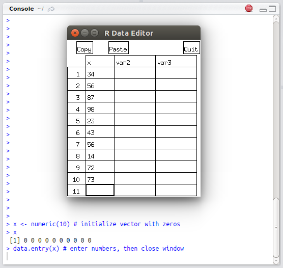
FIGURE 4.1: Example of using the data.entry function in RStudio console
However, the edit function applied to a vector does not open a
spreadsheet. Try the edit function and see what happens.
To enter data into a spreadsheet matrix, first initialize a matrix and
then use the data.entry or edit function. Notice that the editor
added default column names. However, to add our own column names just
click on the column heading with our mouse pointer (unfortunately we
cannot give row names).
xnew <- matrix(numeric(4),2,2)
data.entry(xnew)
xnew <- edit(xnew) #equivalent

#### open spreadsheet editor in one step
xnew <- edit(matrix(numeric(4),2,2)); xnew
#>      col1 col2
#> [1,]   11   33
#> [2,]   22   44
Arrays and nontabular lists cannot be entered using a spreadsheet
editor. Hence, we begin to see the limitations of spreadsheet-type
approach to data entry. One type of list, the data frame, can be
entered using the edit function.
To enter a data frame use the edit function. However, we do not need
to initialize a data frame (unlike with a matrix). Again, click on the
column headings to enter column names.
df <- edit(data.frame()) # spreadsheet screen not shown
df
#>     mykids  age
#> 1 Tomasito   17
#> 2  Luisito   16
#> 3 Angelita   13
When using the edit function to create a new data frame we must
assign it an object name to save the data frame. Later we will see
that when we edit an existing data object we can use the edit or
fix function. The fix function differs in that
fix(data_object) saves our edits directly back to data_object
without the need to make a new assignment.
4.1.2 Importing data from a file
4.1.2.1 Reading an ASCII text data file
In this section we review how to read the following types of text data files:
- Comma-separated variable (csv) data file (\(\pm\) headers and \(\pm\) row names)
- Fixed width formatted data file (\(\pm\) headers and \(\pm\) row names)
Here is the University Group Diabetes Program randomized clinical trial text data file that is comma-delimited, and includes row names and a header (ugdp.txt).20 The header is the first line that contains the column (field) names. The row names is the first column that starts on the second line and uniquely identifies each row. Notice that the row names do not have a column name associated with it. A data file can come with either row names or header, neither, or both. Our preference is to work with data files that have a header and data values that are self-explanatory. Even without a data dictionary one can still make sense out of this data set.
Status,Treatment,Agegrp
1,Dead,Tolbutamide,<55
2,Dead,Tolbutamide,<55
...
408,Survived,Placebo,55+
409,Survived,Placebo,55+
Notice that the header row has 3 items (field names), and the second row has 4
items. This is because the row names start in the second row and have
no column name. This data file can be read in using the read.table
function, and R figures out that the first column are row
names.21 Here we read
in and display the first four lines of this data set:
udat1 <- read.table('~/data/ugdp1.txt', header = TRUE, sep = ",")
udat1[1:4,] # display first 4 lines
#> Status Treatment Agegrp
#> 1 Death Tolbutamide <55
#> 2 Death Tolbutamide <55
#> 3 Death Tolbutamide <55
#> 4 Death Tolbutamide <55Next (below) is the same data (ugdp2.txt) but without a header and
without row names:
And here is how we read this comma-delimited data set (ugdp2.txt):
cnames <- c('Status', 'Treatment', 'Agegrp')
udat2 <- read.table('~/data/ugdp2.txt', header = FALSE, sep = ",",
                    col.names = cnames)
udat2[1:4,] # display first 4 lines
#> Status Treatment Agegrp
#> 1 Dead Tolbutamide <55
#> 2 Dead Tolbutamide <55
#> 3 Dead Tolbutamide <55
#> 4 Dead Tolbutamide <55Here is the same data (ugdp3.txt) as a fix formatted file. In this
file, columns 1 to 8 are for field #1, columns 9 to 19 are for field
#2, and columns 20 to 22 are for field #3. This type of data file is
more compact. One needs a data dictionary to know which columns
contain which fields.
Dead    Tolbutamide<55
...
Dead    Tolbutamide55+
...
Dead    Placebo    <55
...
SurvivedTolbutamide<55
...
SurvivedPlacebo    <55
...
SurvivedPlacebo    55+
This data file would be read in using the read.fwf
function. Because the field widths are fixed, we must strip the white
space using the strip.white option.
cnames <- c('Status', 'Treatment', 'Agegrp')
udat3 <- read.fwf('~/data/ugdp3.txt', width = c(8, 11, 3),
                   col.names = cnames, strip.white = TRUE)
udat3[1:4,]
#> Status Treatment Agegrp
#> 1 Dead Tolbutamide <55
#> 2 Dead Tolbutamide <55
#> 3 Dead Tolbutamide <55
#> 4 Dead Tolbutamide <55Finally, here is the same data file as a fixed width formatted file
but with integer codes (ugdp4.txt). In this file, column 1 is for
field #1, column 2 is for field #2, and column 3 is for field #3. This
type of text data file is the most compact, however, one needs a data
dictionary to make sense of all the 1s and 2s.
Here is how this data file would be read in using the
read.fwf function.
cnames <- c('Status', 'Treatment', 'Agegrp')
udat4 <- read.fwf('~/data/ugdp4.txt', width = c(1, 1, 1),
                  col.names = cnames)
udat4[1:4,]
#> Status Treatment Agegrp
#> 1 1 2 1
#> 2 1 2 1
#> 3 1 2 1
#> 4 1 2 1R has other functions for reading text data files (read.csv,
read.csv2, read.delim, read.delim2). In general, read.table is
the function used most commonly for reading in data files.
4.1.2.2 Reading data from a binary format (e.g., Stata)
To read data that comes in a binary or proprietary format load the
foreign package using the library function. To review available
functions in the the foreign package try help(package = foreign).
For example, here we read in the infert data set which is also
available as a Stata data file.
#>   id education age parity induced case spontaneous
#> 1  1         0  26      6       1    1           2
#> 2  2         0  42      1       1    1           0
#> 3  3         0  39      6       2    1           0
#> 4  4         0  34      4       2    1           0
4.1.3 Importing data using a URL
As we have already seen, text data files can be read directly off a
web server into R using read.table or equivalent
function.
4.2 Editing data
In the ideal setting, our data has already been checked, errors corrected, and ready to be analyzed. Post-collection data editing can be minimized by good design and data collection. However, we may still need to make corrections or changes in data values.
4.2.1 Text editor
Figure 4.2 displays West Nile virus (WNV) infection surveillance data in the GNU Emacs text editor.22 In RStudio, this is equivalent to the script editor (left upper window), and the console (left lower window).
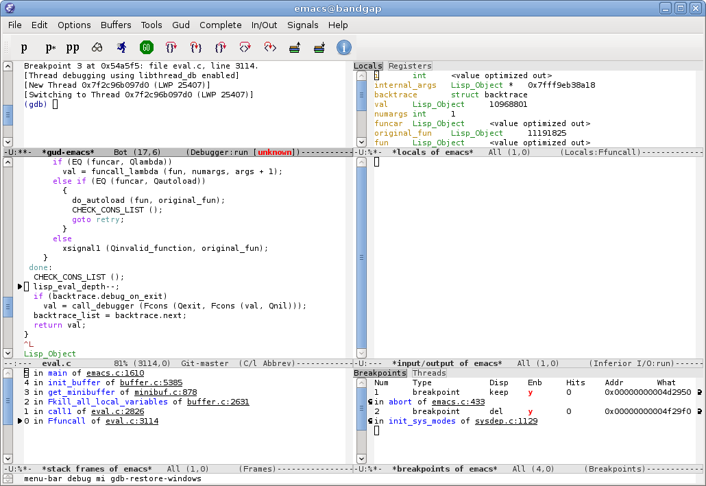
FIGURE 4.2: Left frame: Editing West Nile virus human surveillance data in GNU Emacs text editor. Right frame: Running R using Emacs Speaks Statistics (ESS). Data source: California Department of Health Services, 2004
4.2.2 The data.entry, edit, or fix functions
For vector and matrices we can use the data.entry function to
edit these data object elements. For data frames and functions use
the edit or fix functions. Remember that changes
made with the edit function are not saved unless we assign it
to the original or new object name. In contrast, changes made with
the fix function are saved back to the original data object
name. Therefore, be careful when we use the fix function
because we may unintentionally overwrite data.
Now let’s read in the WNV surveillance raw data as a data frame.
Then, using the fix function, we will edit the first three
records where the value for the syndome variable is “Unknown” and
change it to NA for missing. We will also change “.” to NA.
wd <- read.table('~/data/wnv/wnv2004raw.csv', header = TRUE,
                 sep = ",",  as.is = TRUE)
wd[wd$syndrome=='Unknown',][1:3, -7]  # before edits

#>      id      county age sex syndrome date.onset death
#> 128 128 Los Angeles  81   M  Unknown 07/28/2004     .
#> 129 129   Riverside  44   F  Unknown 07/25/2004     .
#> 133 133 Los Angeles  36   M  Unknown 08/04/2004    No

fix(wd) # opens R data editor and edits made -- not shown
wd[c(128, 129, 133), -7]  # after edits (3 records)

#>      id      county age sex syndrome date.onset death
#> 128 128 Los Angeles  81   M       NA 07/28/2004    NA
#> 129 129   Riverside  44   F       NA 07/25/2004    NA
#> 133 133 Los Angeles  36   M       NA 08/04/2004    No
First, notice that in the read.table function as.is=TRUE. This
means the data is read in without R making any changes to it. In
other words, character vectors are not automatically converted to
factors. We set the option because we knew we were going to edit and
make corrections to the data set, and create factors later. In this
example, we manually changed the missing values “Unknown” to NA (R’s
representation of missing values). However, the manual approach is
very inefficient. A better approach is to specify which values in the
data frame should be converted to NA. In the read.table function we
can set the option na.string = c('Unknown', '.'), converting the
character strings “Unknown” and “.” into NA. Let’s replace the
missing values with NAs upon reading the data file.
wd <- read.table('~/data/wnv/wnv2004raw.csv', header = TRUE,
             sep = ",", as.is = TRUE, na.string=c('Unknown', '.'))
wd[c(128, 129, 133),]  # verify change
#> id county age sex syndrome date.onset date.tested
#> 128 128 Los Angeles 81 M <NA> 07/28/2004 08/11/2004
#> 129 129 Riverside 44 F <NA> 07/25/2004 08/11/2004
#> 133 133 Los Angeles 36 M <NA> 08/04/2004 08/11/2004
#> death
#> 128 <NA>
#> 129 <NA>
#> 133 No4.2.3 Vectorized approach
How do we make these and other changes after the data set has been read into R? Although using R’s spreadsheet function is convenient, we do not recommend it because manual editing is inefficient, our work cannot be replicated and audited, and documentation is poor. Instead use R’s vectorized approach. Let’s look at the distribution of responses for each variable to assess what needs to be “cleaned up,” in addition to converting missing values to NA. We use the following code to read in (again) and evaluate the raw data.
#> 'data.frame':    779 obs. of  8 variables:
#>  $ id         : int  1 2 3 4 5 6 7 8 9 10 ...
#>  $ county     : chr  "San Bernardino" "San Bernardino" "San Bernardino" "San Bernardino" ...
#>  $ age        : chr  "40" "64" "19" "12" ...
#>  $ sex        : chr  "F" "F" "M" "M" ...
#>  $ syndrome   : chr  "WNF" "WNF" "WNF" "WNF" ...
#>  $ date.onset : chr  "05/19/2004" "05/22/2004" "05/22/2004" "05/16/2004" ...
#>  $ date.tested: chr  "06/02/2004" "06/16/2004" "06/16/2004" "06/16/2004" ...
#> $ death : chr "No" "No" "No" "No" ...#> $county
#>
#> Butte Fresno Glenn Imperial
#> 7 11 3 1
#> Kern Lake Lassen Los Angeles
#> 59 1 1 306
#> Merced Orange Placer Riverside
#> 1 62 1 109
#> Sacramento San Bernardino San Diego San Joaquin
#> 3 187 2 2
#> Santa Clara Shasta Sn Luis Obispo Tehama
#> 1 5 1 10
#> Tulare Ventura Yolo
#> 3 2 1
#>
#> $age
#>
#> . 1 10 11 12 13 14 15 16 17 18 19 2 20 21 22 23 24 25 26 27
#> 6 1 1 1 3 2 3 3 1 4 6 5 1 4 2 3 6 8 3 9 4
#> 28 29 30 31 32 33 34 35 36 37 38 39 4 40 41 42 43 44 45 46 47
#> 8 1 8 6 3 6 15 15 8 8 5 7 1 9 17 15 19 11 14 23 25
#> 48 49 5 50 51 52 53 54 55 56 57 58 59 6 60 61 62 63 64 65 66
#> 19 22 2 14 16 24 17 14 17 13 16 8 17 2 29 13 15 7 12 10 7
#> 67 68 69 7 70 71 72 73 74 75 76 77 78 79 8 80 81 82 83 84 85
#> 8 8 14 2 12 10 9 11 12 7 10 7 7 7 1 6 11 10 5 6 4
#> 86 87 88 89 9 91 93 94
#> 2 2 1 6 1 4 1 1
#>
#> $sex
#>
#> . F M
#> 2 294 483
#>
#> $syndrome
#>
#> Unknown WNF WNND
#> 105 391 283
#>
#> $death
#>
#> . No Yes
#> 66 686 27What did we learn? First, there are 779 observations and 781 id’s; therefore, three observations were removed from the original data set. Second, we see that the variables age, sex, syndrome, and death have missing values that need to be converted to NAs. This can be done one field at a time, or for the whole data frame in one step. Here is the R code:
wd$age[wd$age=='.'] <- NA
wd$sex[wd$sex=='.'] <- NA
wd$syndrome[wd$syndrome == 'Unknown'] <- NA
wd$death[wd$death=='.'] <- NA
table(wd$death)  # verify
#>
#> No Yes
#> 686 27#>
#> No Yes <NA>
#> 686 27 66Note that the NA replacement could have been done globally like this:
We also notice that the entry for one of the counties, San Luis
Obispo, was misspelled (Sn Luis Obispo). We can use
replacement to correct this:
4.2.4 Text processing
On occasion, we will need to process and manipulate character vectors
using a vectorized approach. For example, suppose we need to convert
a character vector of dates from “mm/dd/yy” to
“yyyy-mm-dd.”23
We’ll start by using the substr function. This function extracts
characters from a character vector based on position.
#> [1] "07" "12" "11"#> [1] "17" "09" "07"#> [1] 96 0 97#> [1] 1996 2000 1997#> [1] "1996-07-17" "2000-12-09" "1997-11-07"In this example, we needed to convert “00” to “2000”, and “96”
and “97” to “1996” and “1997”, respectively. The trick here was
to coerce the character vector into a numeric vector so that 1900 or
2000 could be added to it. Using the ifelse function, for
values \(\le 19\) (arbitrarily chosen), 2000 was added, otherwise 1900
was added. The paste function was used to paste back the
components into a new vector with the standard date format.
The substr function can also be used to replace characters in
a character vector. Remember, if it can be indexed, it can be
replaced.
#> [1] "07/17/96" "12/09/00" "11/07/97"#> [1] "07-17-96" "12-09-00" "11-07-97"| Function | Description with examples |
|---|---|
nchar |
Returns the number of characters in each element of a character vector |
x = c('a', 'ab', 'abc', 'abcd'); nchar(x) |
|
substr |
Extract or replace substrings in a character vector |
#### extraction |
|
mon = substr(some.dates, 1, 2); mon |
|
day = substr(some.dates, 4, 5); day |
|
yr = substr(some.dates, 7, 8); yr |
|
#### replacement |
|
mdy = paste(mon, day, yr); mdy |
|
substr(mdy, 3, 3) = '/' |
|
substr(mdy, 6, 6) = '/'; mdy |
|
paste |
Concatenate vectors after converting to character |
rd = paste(mon, '/', day, '/', yr, sep=""); rd |
|
strsplit |
Split the elements of a character vector into substrings |
some.dates = c('10/02/70', '02/04/67') |
|
strsplit(some.dates, '/') |
4.3 Sorting data
The sort function sorts a vector as expected:
#> [1] 3 4 6 5 1 7 8 9 2 10#> [1] 1 2 3 4 5 6 7 8 9 10#> [1] 10 9 8 7 6 5 4 3 2 1#> [1] 10 9 8 7 6 5 4 3 2 1However, if we want to sort one vector based on the ordering of
elements from another vector, use the order function. The order
function generates an indexing/repositioning vector. Study the
following example:
#> [1] 7 8 15 16 20#> [1] 5 1 4 3 2#> [1] 8 15 16 20 7Based on this we can see that sort(x) is just
x[order(x)].
Now let us see how to use the order function for data frames.
First, we create a small data set.
sex <- rep(c('Male', 'Female'), c(4, 4))
ethnicity <- rep(c('White', 'Black', 'Latino', 'Asian'), 2)
age <- c(57, 93, 7, 65, 38, 27, 66, 72)
dat <- data.frame(age, sex, ethnicity)
dat <- dat[sample(1:8, 8), ] # randomly order rows
dat
#> age sex ethnicity
#> 1 57 Male White
#> 2 93 Male Black
#> 6 27 Female Black
#> 4 65 Male Asian
#> 5 38 Female White
#> 7 66 Female Latino
#> 8 72 Female Asian
#> 3 7 Male LatinoOkay, now we will sort the data frame based on the ordering of one field, and then the ordering of two fields:
#>   age    sex ethnicity
#> 3   7   Male    Latino
#> 6  27 Female     Black
#> 5  38 Female     White
#> 1  57   Male     White
#> 4  65   Male     Asian
#> 7  66 Female    Latino
#> 8  72 Female     Asian
#> 2 93 Male Black#> age sex ethnicity
#> 6 27 Female Black
#> 5 38 Female White
#> 7 66 Female Latino
#> 8 72 Female Asian
#> 3 7 Male Latino
#> 1 57 Male White
#> 4 65 Male Asian
#> 2 93 Male Black4.4 Indexing (subsetting) data
In R, we use indexing to subset (or extract) parts of a data object. For this section, please load the well known Oswego foodborne illness data frame using:
odat <- read.table('~/data/oswego/oswego.txt', header = TRUE,
                   as.is = TRUE, sep = "")
names(odat) # display field names
#> [1] "id" "age" "sex"
#> [4] "meal.time" "ill" "onset.date"
#> [7] "onset.time" "baked.ham" "spinach"
#> [10] "mashed.potato" "cabbage.salad" "jello"
#> [13] "rolls" "brown.bread" "milk"
#> [16] "coffee" "water" "cakes"
#> [19] "van.ice.cream" "choc.ice.cream" "fruit.salad"4.4.1 Indexing
Now, we practice indexing rows from this data frame. First, we create
a new data set that contains only cases. To index the rows with cases
we need to generate a logical vector that is TRUE for every value of
odat$ill that is equivalent to'' `'Y'`. Foris equivalent to’’
we use the == relational operator.
cases <- odat$ill=='Y'  # logical vector to index cases
odat.ca <- odat[cases, ]
odat.ca[1:4, 1:7] # display part of data set
#> id age sex meal.time ill onset.date onset.time
#> 1 2 52 F 8:00 PM Y 4/19 12:30 AM
#> 2 3 65 M 6:30 PM Y 4/19 12:30 AM
#> 3 4 59 F 6:30 PM Y 4/19 12:30 AM
#> 4 6 63 F 7:30 PM Y 4/18 10:30 PMIt is very important to understand what we just did: we extracted the rows with cases by indexing the data frame with a logical vector.
Now, we combine relational operators with logical operators to extract rows based on multiple criteria. Let’s create a data set with female cases, age less than the median age, and consumed vanilla ice cream.
fem.cases.vic <- odat$ill == 'Y' & odat$sex == 'F' &
    odat$van.ice.cream == 'Y' & odat$age < median(odat$age)
odat.fcv <- odat[fem.cases.vic, ]
odat.fcv[ , c(1:6, 19)]
#> id age sex meal.time ill onset.date van.ice.cream
#> 8 10 33 F 7:00 PM Y 4/18 Y
#> 10 16 32 F <NA> Y 4/19 Y
#> 13 20 33 F <NA> Y 4/18 Y
#> 14 21 13 F 10:00 PM Y 4/19 Y
#> 18 27 15 F 10:00 PM Y 4/19 Y
#> 23 36 35 F <NA> Y 4/18 Y
#> 31 48 20 F 7:00 PM Y 4/19 Y
#> 37 58 12 F 10:00 PM Y 4/19 Y
#> 40 65 17 F 10:00 PM Y 4/19 Y
#> 41 66 8 F <NA> Y 4/19 Y
#> 42 70 21 F <NA> Y 4/19 Y
#> 44 72 18 F 7:30 PM Y 4/19 YIn summary, we see that indexing rows of a data frame consists of
using relational operators (<, >, <=, >=, ==, !=) and logical
operators (&, |, !) to generate a logical vector for indexing the
appropriate rows.
4.4.2 Using the subset function
Indexing a data frame using the subset function is equivalent to
using logical vectors to index the data frame. In general, we prefer
indexing because it is generalizable to indexing any R data object.
However, the subset function is a convenient alternative for data
frames. Again, let’s create data set with female cases, age \(<\)
median, and ate vanilla ice cream.
odat.fcv <- subset(odat, subset = {ill == 'Y' & sex == 'F' &
             van.ice.cream == 'Y' & age < median(odat$age)},
                   select = c(id:onset.date, van.ice.cream))
odat.fcv
#> id age sex meal.time ill onset.date van.ice.cream
#> 8 10 33 F 7:00 PM Y 4/18 Y
#> 10 16 32 F <NA> Y 4/19 Y
#> 13 20 33 F <NA> Y 4/18 Y
#> 14 21 13 F 10:00 PM Y 4/19 Y
#> 18 27 15 F 10:00 PM Y 4/19 Y
#> 23 36 35 F <NA> Y 4/18 Y
#> 31 48 20 F 7:00 PM Y 4/19 Y
#> 37 58 12 F 10:00 PM Y 4/19 Y
#> 40 65 17 F 10:00 PM Y 4/19 Y
#> 41 66 8 F <NA> Y 4/19 Y
#> 42 70 21 F <NA> Y 4/19 Y
#> 44 72 18 F 7:30 PM Y 4/19 YIn the subset function, the first argument is the data frame object
name, the second argument (also called subset) evaluates to a
logical vector, and third argument (called select) specifies the
fields to keep. In the second argument, subset = {...}, the curly
brackets are included for convenience to group the logical and
relational operations. In the select argument, using the :
operator, we can specify a range of fields to keep.
4.5 Transforming data
Transforming fields in a data frame is very common. The most common transformations include the following:
- Numerical transformation of a numeric vector
- Discretizing a numeric vector into categories or levels (“categorical variable”)
- Recoding factor levels (categorical variables)
For each of these, we must decide whether the newly created vector should be a new field in the data frame, overwrite the original field in the data frame, or not be a field in the data frame (but rather a vector object in the R workspace). For the examples that follow load the well known Oswego foodborne illness dataset:
4.5.1 Numerical transformation
In this example we “center” the age field by substracting
the mean age from each age.
#>    Min. 1st Qu.  Median    Mean 3rd Qu.    Max.
#>    3.00   16.50   36.00   36.81   57.50   77.00
#### create new field in same data frame
odat$age.centered <- odat$age - mean(odat$age)
summary(odat$age.centered)#> Min. 1st Qu. Median Mean 3rd Qu. Max.
#> -33.8133 -20.3133 -0.8133 0.0000 20.6867 40.1867#### create new vector in workspace; data frame unchanged
age.centered <- odat$age - mean(odat$age)
summary(age.centered)#> Min. 1st Qu. Median Mean 3rd Qu. Max.
#> -33.8133 -20.3133 -0.8133 0.0000 20.6867 40.1867For convenience, the transform function facilitates the
transformation of numeric vectors in a data frame. The transform
function comes in handy when we plan on transforming many fields: we
do not need to specify the data frame each time we refer to a field
name. For example, the following lines are are equivalent. Both add
a new transformed field to the data frame.
odat$age.centered <- odat$age - mean(odat$age)
odat <- transform(odat, age.centered = age - mean(age))
TODO
4.5.2 Recoding vector values
4.5.2.1 Recoding using replacement
Here is a straightforward example of recoding a vector by replacement:
x <- c("m", "f", "u", "f", "f", "m", "m")
y <- x  # create copy
y[x=="m"] <- "Male"
y[x=="f"] <- "Female"
y[x=="u"] <- NA
table(y)
#> y
#> Female Male
#> 3 34.5.2.2 Recoding using a lookup table
Alternatively, we can use character matching to create a lookup table which is just indexing by name (or the data character vector).
#>        m        f        u        f        f        m        m
#>   "Male" "Female"       NA "Female" "Female"   "Male"   "Male"
Note that if you don’t want names in the result, use unname() to remove them.
#> [1] "Male"   "Female" NA       "Female" "Female" "Male"
#> [7] "Male"
4.5.3 Creating categorical variables (factors)
Now, reload the Oswego data set to recover the original odat$age
field. We are going to create a new field with the following six age
categories (in years): <5, 5 to 14, 15 to 24, 25 to 44, 45 to 64, and 65+. We will demonstrate this using several methods.
4.5.3.1 Using cut function (preferred method)
Here we use the cut function.
#> agecat
#>    (0,5]   (5,15]  (15,25]  (25,45]  (45,65] (65,100]
#>        1       17       12       17       22        6
Note that the cut function generated a factor with
7 levels for each interval. The notation (15, 25] means that
the interval is open on the left boundary (>15) and closed on the
right boundary (\(\le 25\)). However, in the United States, for age
categories, the age boundaries are closed on the left and open on the
right: [a, b). To change this we set the option
right = FALSE
#> agecat
#>    [0,5)   [5,15)  [15,25)  [25,45)  [45,65) [65,100)
#>        1       14       13       18       20        9
Okay, this looks good, but we can add labels since our readers may not be familiar with open and closed interval notation \([a, b)\).
agelabs <- c('<5', '5-14', '15-24', '25-44', '45-64', '65+')
agecat <- cut(odat$age, breaks = c(0, 5, 15, 25, 45,
    65, 100), right = FALSE, labels = agelabs)
table(Illness = odat$ill, 'Age category' = agecat) # display
#> Age category
#> Illness <5 5-14 15-24 25-44 45-64 65+
#> N 0 8 5 8 5 3
#> Y 1 6 8 10 15 64.5.3.2 Using indexing and assignment (replacement)
The cut function is the preferred method to create a
categorical variable. However, suppose one does not know about the
cut function. Applying basic R concepts always works!
agecat <- odat$age
agecat[odat$age < 5] <- 1
agecat[odat$age >= 5 & odat$age < 15] <- 2
agecat[odat$age >= 15 & odat$age < 25] <- 3
agecat[odat$age >= 25 & odat$age < 45] <- 4
agecat[odat$age >= 45 & odat$age < 65] <- 5
agecat[odat$age >= 65] <- 6
#### create factor
agelabs <- c('<5', '5-14', '15-24', '25-44', '45-64', '65+')
agecat <- factor(agecat, levels = 1:6, labels = agelabs)
table(Illness = odat$ill, 'Age category' = agecat) # display
#> Age category
#> Illness <5 5-14 15-24 25-44 45-64 65+
#> N 0 8 5 8 5 3
#> Y 1 6 8 10 15 6In these previous examples, notice that agecat is a factor
object in the workspace and not a field in the odat data
frame.
4.5.4 Recoding factor levels (categorical variables)
In the previous example the categorical variable was a numeric vector (1, 2, 3, 4, 5, 6) that was converted to a factor and provided labels (‘<5’, ‘5-14’, …). In fact, categorical variables are often represented by integers (for example, 0 = no, 1 = yes; or 0 = non-case, 1 = case) and provided labels. Often, ASCII text data files are integer codes that require a data dictionary to convert these integers into categorical variables in a statistical package. In R, keeping track of integer codes for categorical variables is unnecessary. Therefore, re-coding the underlying integer codes is also unnecessary; however, if we feel the need to do so, here’s how:
#### Create categorical variable
ethlabs <- c('White', 'Black', 'Latino', 'Asian')
ethnicity <- sample(ethlabs, 100, replace = TRUE)
ethnicity <- factor(ethnicity, levels = ethlabs)
table(ethnicity) # display frequency
#> ethnicity
#> White Black Latino Asian
#> 31 25 23 21The levels option allowed us to determine the display order, and the
first level becomes the reference level in statistical models. To
display the underlying numeric code use unclass function which
preserves the levels
attribute.24
#> ethcode
#> 1 2 3 4
#> 31 25 23 21#> [1] "White" "Black" "Latino" "Asian"To recover the original factor,
#> eth.orig
#> White Black Latino Asian
#> 31 25 23 21Although we can extract the integer code, why would we need to do so? One is tempted to use the integer codes as a way to share data sets. However, we recommend not using the integer codes, but rather just provide the data in its native format.25 This way, the raw data is more interpretable and eliminates the intermediate step of needing to label the integer code. Also, if the data dictionary is lost or not provided, the raw data is still interpretable.
In R, we can re-label the levels using the levels function
and assigning to it a character vector of new labels. Make sure the
order of the new labels corresponds to the order of the factor levels.
#> [1] "White" "Black" "Latino" "Asian"eth2 <- ethnicity # create duplicate
levels(eth2) <- c('Caucasion', 'Afr. American', 'Hispanic', 'Asian') # assign new levels
table(eth2) # display frequency with new levels#> eth2
#> Caucasion Afr. American Hispanic Asian
#> 31 25 23 21In R, we can re-order and re-label at the same time using the
levels function and assigning to it a list. The
list function is necessary to assure the re-ordering.
eth3 <- ethnicity # create duplicate
levels(eth3) <- list(Hispanic = 'Latino', Asian = 'Asian',
Caucasion = 'White', 'Afr. American' = 'Black')
table(eth3) # display frequency with new levels & labels#> eth3
#> Hispanic Asian Caucasion Afr. American
#> 23 21 31 25To re-order without re-labeling use the list function
#> ethnicity
#>  White  Black Latino  Asian
#> 31 25 23 21eth4 <- ethnicity
levels(eth4) <- list(Latino = 'Latino', Asian = 'Asian',
White = 'White', Black = 'Black')
table(eth4)#> eth4
#> Latino Asian White Black
#> 23 21 31 25In R, we can sort the factor levels by using the factor
function in one of two ways:
#> ethnicity
#>  White  Black Latino  Asian
#> 31 25 23 21#> eth5a
#> Asian Black Latino White
#> 21 25 23 31#> eth5b
#> Asian Black Latino White
#> 21 25 23 31In the first example, we assigned to the levels
argument the sorted level names. In the second example, we started
from scratch by coercing the original factor into a character vector
which is then ordered alphabetically by default.
4.5.4.1 Setting factor reference level
The first level of a factor is the reference level for some
statistical models (e.g., logistic regression). To set a different
reference level use the relevel function.%
#> [1] "White" "Black" "Latino" "Asian"#> [1] "Asian" "White" "Black" "Latino"As we can see, there is tremendous flexibility in dealing with factors without the need to ``re-code’’ categorical variables. This approach facilitates reviewing our work and minimizes errors.
4.5.5 Use factors instead of dummy variables
| Factor | Dummy | variable | codes |
|---|---|---|---|
| Ethnicity | Asian | Black | Latino |
| White | 0 | 0 | 0 |
| Asian | 1 | 0 | 0 |
| Black | 0 | 1 | 0 |
| Latino | 0 | 0 | 1 |
A nonordered factor (nominal categorical variable) with \(k\) levels can
also be represented with \(k-1\) dummy variables. For example, the
ethnicity factor has four levels: white, Asian, black, and
Latino. Ethnicity can also be represented using 3 dichotomous
variables, each coded 0 or 1. For example, using white as the
reference group, the dummy variables would be asian,
black, and latino (see Table 4.3). The
values of those three dummy variables (0 or 1) are sufficient to
represents one of four possible ethnic categories. Dummy variables
can be used in statistical models. However, in R, it is unnecessary to
create dummy variables, just create a factor with the desired number
of levels and set the reference level.
4.5.6 Conditionally transforming the elements of a vector
We can conditionally transform the elements of a vector using the
ifelse function. This function works as follows:
ifelse(test, if test = TRUE do this, else do this)
#> [1] "F" "M" "F" "F" "M" "F" "F" "M" "M" "F"#> [1] "Female" "Male" "Female" "Female" "Male" "Female"
#> [7] "Female" "Male" "Male" "Female"| Function | Description | Try these examples |
|---|---|---|
<- |
Transforming a vector and assigning it to a new data frame variable name | dat <- data.frame(id=1:3, x=c(0.5,1,2)) |
dat$logx <- log(x) # creates new field |
||
dat |
||
| transform | Transform one or more variables from a data frame | dat <- data.frame(id=1:3, x=c(0.5,1,2)) |
dat <- transform(dat, logx = log(x)) |
||
dat |
||
| cut | Creates a factor by dividing the range of a numeric vector into intervals | age <- sample(1:100, 500, replace = TRUE) |
#### cut into 2 intervals |
||
agecut <- cut(age, 2, right = FALSE) |
||
table(agecut) |
||
#### cut using specified intervals |
||
agecut2 <- cut(age, c(0, 50 100),right = FALSE, include.lowest = TRUE) |
||
table(agecut2) |
||
| levels | Gives access to the levels attribute of a factor | sex <- sample(c('M','F','T'),500, replace=T) |
sex <- factor(sex) |
||
table(sex) |
||
#### relabel each level; use same order |
||
levels(sex) <- c('Female', 'Male', 'Transgender') |
||
table(sex) |
||
#### relabel/recombine |
||
levels(sex) <- c('Female', 'Male', 'Male') |
||
table(sex) |
||
#### reorder and/or relabel |
||
levels(sex) <- list ('Men' = 'Male', 'Women' = 'Female') |
||
table(sex) |
||
| relevel | Set the reference level for a factor | sex2 <- relevel(sex, ref = 'Women') |
table(sex2) |
||
| ifelse | Conditionally operate on elements of a vector based on a test | age <- sample(1:100, 1000, replace = TRUE) |
agecat <- ifelse(age<=50, '<=50', '>50') |
||
table(agecat) |
4.6 Merging data
In general, R’s strength is not data management but rather data analysis. Because R can access and operate on multiple objects in the workspace it is generally not necessary to merge data objects into one data object in order to conduct analyses. On occasion, it may be necessary to merge two data frames into one data frames
Data frames that contain data on individual subjects are generally of two types: (1) each row contains data collected on one and only one individual, or (2) multiple rows contain repeated measurements on individuals. The latter approach is more efficient at storing data. For example, here are two approaches to collecting multiple telephone numbers for two individuals.
#>             name   wphone   fphone   mphone
#> 1   Tomas Aragon 643-4935 643-2926 847-9139
#> 2 Wayne Enanoria 643-4934 <NA> <NA>#> name telephone teletype
#> 1 Tomas Aragon 643-4935 Work
#> 2 Tomas Aragon 643-2926 Fax
#> 3 Tomas Aragon 847-9139 Mobile
#> 4 Wayne Enanoria 643-4934 WorkThe first approach is represented by tab1, and the second approach
by
tab2.26
Data is more efficiently stored in tab2, and adding new types of
telephone numbers only requires assigning a new value (e.g., Pager) to
the teletype field.
#>             name telephone teletype
#> 1   Tomas Aragon  643-4935     Work
#> 2   Tomas Aragon  643-2926      Fax
#> 3   Tomas Aragon  847-9139   Mobile
#> 4 Wayne Enanoria  643-4934     Work
#> 5 Tomas Aragon 719-1234 PagerIn both these data frames, an indexing field identifies an unique
individual that is associated with each row. In this case, the name
column is the indexing field for both data frames.
Now, let’s look at an example of two related data frames that are
linked by an indexing field. The first data frame contains telephone
numbers for 5 employees and fname is the indexing field. The second
data frame contains email addresses for 3 employees and name is the
indexing field.
#>    fname phonenum phonetype
#> 1  Tomas 643-4935      work
#> 2  Tomas 847-9139    mobile
#> 3  Tomas 643-4926       fax
#> 4  Chris 643-3932      work
#> 5  Chris 643-4926       fax
#> 6  Wayne 643-4934      work
#> 7  Wayne 643-4926       fax
#> 8    Ray 643-4933      work
#> 9    Ray 643-4926       fax
#> 10 Diana 643-3931 work#> name mail mailtype
#> 1 Tomas aragon@berkeley.edu Work
#> 2 Tomas aragon@medepi.net Personal
#> 3 Wayne enanoria@berkeley.edu Work
#> 4 Wayne enanoria@idready.org Work
#> 5 Chris cvsiador@berkeley.edu Work
#> 6 Chris cvsiador@yahoo.com PersonalTo merge these two data frames use the merge function. The by.x
and by.y options identify the indexing fields.
#>    fname phonenum phonetype                  mail mailtype
#> 1  Chris 643-3932      work cvsiador@berkeley.edu     Work
#> 2  Chris 643-3932      work    cvsiador@yahoo.com Personal
#> 3  Chris 643-4926       fax cvsiador@berkeley.edu     Work
#> 4  Chris 643-4926       fax    cvsiador@yahoo.com Personal
#> 5  Tomas 643-4926       fax   aragon@berkeley.edu     Work
#> 6  Tomas 643-4926       fax     aragon@medepi.net Personal
#> 7  Tomas 643-4935      work   aragon@berkeley.edu     Work
#> 8  Tomas 643-4935      work     aragon@medepi.net Personal
#> 9  Tomas 847-9139    mobile   aragon@berkeley.edu     Work
#> 10 Tomas 847-9139    mobile     aragon@medepi.net Personal
#> 11 Wayne 643-4926       fax enanoria@berkeley.edu     Work
#> 12 Wayne 643-4926       fax  enanoria@idready.org     Work
#> 13 Wayne 643-4934      work enanoria@berkeley.edu     Work
#> 14 Wayne 643-4934      work  enanoria@idready.org     Work
By default, R selects the rows from the two data frames that is based
on the intersection of the indexing fields (by.x, by.y). To
merge the union of the indexing fields, set all=TRUE:
#>    fname phonenum phonetype                  mail mailtype
#> 1  Chris 643-3932      work cvsiador@berkeley.edu     Work
#> 2  Chris 643-3932      work    cvsiador@yahoo.com Personal
#> 3  Chris 643-4926       fax cvsiador@berkeley.edu     Work
#> 4  Chris 643-4926       fax    cvsiador@yahoo.com Personal
#> 5  Diana 643-3931      work                  <NA>     <NA>
#> 6    Ray 643-4926       fax                  <NA>     <NA>
#> 7    Ray 643-4933      work                  <NA>     <NA>
#> 8  Tomas 643-4926       fax   aragon@berkeley.edu     Work
#> 9  Tomas 643-4926       fax     aragon@medepi.net Personal
#> 10 Tomas 643-4935      work   aragon@berkeley.edu     Work
#> 11 Tomas 643-4935      work     aragon@medepi.net Personal
#> 12 Tomas 847-9139    mobile   aragon@berkeley.edu     Work
#> 13 Tomas 847-9139    mobile     aragon@medepi.net Personal
#> 14 Wayne 643-4926       fax enanoria@berkeley.edu     Work
#> 15 Wayne 643-4926       fax  enanoria@idready.org     Work
#> 16 Wayne 643-4934      work enanoria@berkeley.edu     Work
#> 17 Wayne 643-4934      work  enanoria@idready.org     Work
%%TODO: MAKE TABLE OF MERGE, STACK, reshape
To `reshape'' tabular data look up and study thereshapeandstack` functions.
4.7 Executing commands from, and directing output to, a file
4.7.1 The source function
The source function is used to evaluate R expressions that
have beenn collected in a R script file. For example, consider the contents
this script file (outer-multiplication-table.R):
Here the source function is used at the R console to “source”
(evaluate and execute) the outer-multiplication-table.R file:
#>       [,1] [,2] [,3] [,4] [,5] [,6] [,7] [,8] [,9] [,10]
#>  [1,]    1    2    3    4    5    6    7    8    9    10
#>  [2,]    2    4    6    8   10   12   14   16   18    20
#>  [3,]    3    6    9   12   15   18   21   24   27    30
#>  [4,]    4    8   12   16   20   24   28   32   36    40
#>  [5,]    5   10   15   20   25   30   35   40   45    50
#>  [6,]    6   12   18   24   30   36   42   48   54    60
#>  [7,]    7   14   21   28   35   42   49   56   63    70
#>  [8,]    8   16   24   32   40   48   56   64   72    80
#>  [9,]    9   18   27   36   45   54   63   72   81    90
#> [10,]   10   20   30   40   50   60   70   80   90   100
Nothing is printed to the console unless we explicitly use
the the show (or print) function. This enables us
to view only the results we want to review.
An alternative approach is to print everything to the console as if
the R commands were being enter directly at the command prompt. For
this we do not need to use the show function in the source
file; however, we must set the echo option to TRUE in the
source function. Here is the edited source file (chap03.R)
Here the source function is used with the option
echo = TRUE:
#>
#> > i <- 1:10
#>
#> > x <- outer(i, i, '*')
#>
#> > x
#>       [,1] [,2] [,3] [,4] [,5] [,6] [,7] [,8] [,9] [,10]
#>  [1,]    1    2    3    4    5    6    7    8    9    10
#>  [2,]    2    4    6    8   10   12   14   16   18    20
#>  [3,]    3    6    9   12   15   18   21   24   27    30
#>  [4,]    4    8   12   16   20   24   28   32   36    40
#>  [5,]    5   10   15   20   25   30   35   40   45    50
#>  [6,]    6   12   18   24   30   36   42   48   54    60
#>  [7,]    7   14   21   28   35   42   49   56   63    70
#>  [8,]    8   16   24   32   40   48   56   64   72    80
#>  [9,]    9   18   27   36   45   54   63   72   81    90
#> [10,]   10   20   30   40   50   60   70   80   90   100
4.7.2 The sink and capture.output functions
To send console output to a separate file use the sink or
capture.output functions. To work correctly, the sink
function is used twice: first, to open a connection to an output
file and, second, to close the connection. By default,
sink creates a new output file. To append to an existing
file set the option append = TRUE. Consider the following
script file (sink-outer.R):
i <- 1:5
x <- outer(i, i, '*')
sink('~/git/phds/example/sink-outer.log') # open connection
cat('Here are results of outer function', fill = TRUE)
show(x)
sink() # close connection
Now the script file (sink-outer.R) is sourced:
Notice that nothing was printed to the console because
sink sent it to the output file. Here are the contents of
sink-outer.log.
Here are results of outer function
     [,1] [,2] [,3] [,4] [,5]
[1,]    1    2    3    4    5
[2,]    2    4    6    8   10
[3,]    3    6    9   12   15
[4,]    4    8   12   16   20
[5,]    5   10   15   20   25
The first sink opened a connection and created the
output file (sink-outer.log). The cat and show functions
printed results to output file. The second sink closed the
connection.
Alternatively, as before, if we use the echo = TRUE option in
the source function, everything is either printed to the
console or output file. The sink connection determines what
is printed to the output file. At the R console, the source
option is set to echo = TRUE:
#>
#> > i <- 1:5
#>
#> > x <- outer(i, i, '*')
#>
#> > sink('~/git/phds/example/sink-outer.log') # open connection
Notice that nothing appears after sink. That is
because the output was redirected to the new output file
sink-outer.log, shown here:
> cat('Here are results of outer function', fill = TRUE)
Here are results of outer function

> show(x)
     [,1] [,2] [,3] [,4] [,5]
[1,]    1    2    3    4    5
[2,]    2    4    6    8   10
[3,]    3    6    9   12   15
[4,]    4    8   12   16   20
[5,]    5   10   15   20   25

> sink() # close connection
The sink and capture.output functions accomplish the
same task: sending results to an output file. The sink
function works in pairs: opening and closing the connection to the
output file. In contrast, capture.output function appears
once and only prints the last object to the output file. Here is the
edited script file (capture-output.R) using
capture.output instead of sink:
i <- 1:5
x <- outer(i, i, '*')
capture.output({
x # display x
}, file = '~/git/phds/example/capture-output.log')
Now the script file is sourced at the R console:
And, here are the contents of capture-output.log:
     [,1] [,2] [,3] [,4] [,5]
[1,]    1    2    3    4    5
[2,]    2    4    6    8   10
[3,]    3    6    9   12   15
[4,]    4    8   12   16   20
[5,]    5   10   15   20   25
Even though the capture.output function can run several R
expressions (between the curly brackets), only the final object
(x) was printed to the output file. This would be true even
if the echo option was not set to TRUE in the source
function.
In summary, the source function evaluates and executes R
expression collected in a script file. Setting the echo
option to TRUE prints expressions and results to the console as if the
commands were directly entered at the command prompt. The
sink and capture.output functions direct results to
an output file.
4.8 Working with missing and “not available” values
In R, missing values are represented by NA, but not all NAs represent missing values—some are just “not available.” NAs can appear in any data object. The NA can represent a true missing value, or it can result from an operation to which a value is “not available.” Here are three vectors that contain true missing values.
#> [1] 2 4 NA 5#> [1] "M" NA "M" "F"#> [1] FALSE NA FALSE TRUEHowever, elementary numerical operations on objects that
contain NA return a single NA (“not available”). In this instance, R
is saying “An answer is ‘not available’ until you tell R what to do
with the NAs in the data object.” To remove NAs for a calculation
specify the na.rm (“NA remove”) option.
#> [1] NA#> [1] NA#> [1] 11#> [1] 3.666667Here are more examples where NA means an answer is not available:
#> Warning: NAs introduced by coercion#> [1] 4 NA#> [1] NA#> v1 v2
#> NA NA NA#> v1 v2
#> NA NA NA#> [1] NA#> [1] NAIn general, these “not available” NAs indicate a missing information issue that must or should be addressed.
4.8.1 Testing, indexing, replacing, and recoding
Regardless of the source of the NAs—missing or not available
values—using the is.na function, we can generate a
logical vector to identify which positions contain or do not contain
NAs. This logical vector can be used index the original or another
vector. Values that can be indexed can be replaced
#> [1] FALSE TRUE FALSE TRUE FALSE#> [1] 2 4#> [1] 10 33 57#> [1] 24 47#> [1] 10 999 33 999 57For a vector, recoding missing values to NA is accomplished using replacement.
#> [1] 1 NA 3 NA 5For a matrix, we can recode missing values to NA by using replacement one column at a time, or globablly like a vector (this is because a matrix is just a reshaped vector).
m <- m2 <- matrix (c(1, -99, 3, 4, -88, 5), 2, 3)
m[m[,1]==-99, 1] <- NA # Replacement one column at a time
m[m[,3]==-88, 3] <- NA; m
#> [,1] [,2] [,3]
#> [1,] 1 3 NA
#> [2,] NA 4 5#> [,1] [,2] [,3]
#> [1,] 1 3 NA
#> [2,] NA 4 5Likewise, for a data frame, we can recode missing values to NA by using replacement one field at a time, or globablly like a vector.
#>     fname  age
#> 1     Tom   56
#> 2 Unknown   34
#> 3 Jerry -999#> fname age
#> 1 Tom 56
#> 2 <NA> 34
#> 3 Jerry NA#> fname age
#> 1 Tom 56
#> 2 <NA> 34
#> 3 Jerry NA4.8.2 Importing missing values with the read.table function
When importing ASCII data files using the read.table
function, use the na.strings option to specify what
characters are to be converted to NA. The default setting is
na.strings = "NA". Blank fields () are also
considered to be missing values in logical, integer, numeric, and
complex fields. For example, suppose the data set contains 999, 888,
., and (space) to represent missing
values, then import the data like this:
If a number, say 999, represents a missing value in one
field but a valid value in another field, then import the data using
the as.is = TRUE option. Then replace the missing values in
the data frame one field at a time, and convert categorical fields to
factors.
4.8.3 Working with NA values in data frames and factors
There are several functions for working with NA values in data
frames. First, the na.fail function tests whether a data frame
contains any NA values, returning an error message if it contains NAs.
#>      name gender age
#> 1    Jose      M  34
#> 2     Ana      F  NA
#> 3 Roberto      M  22
#> 4  Isabel   <NA>  18
#> 5     Jen      F  34
gender <- c("M", "F", "M", NA, "F")
age <- c(34, NA, 22, 18, 34)
df <- data.frame(name, gender, age); df
#> name gender age
#> 1 Jose M 34
#> 2 Ana F NA
#> 3 Roberto M 22
#> 4 Isabel <NA> 18
#> 5 Jen F 34
na.fail(df) # NAs in data frame --- returns error
#> Error in na.fail.default(df) : missing values in object
na.fail(df[c(1, 3, 5),]) # no NAs in data frame
#>      name gender age
#> 1    Jose      M  34
#> 3 Roberto      M  22
#> 5 Jen F 34Both na.omit and na.exclude remove row observations
for any field that contain NAs. The na.exclude differs from
na.omit only in the class of the na.action'' attribute of the result, which isexclude’’ (see help for details).
#>      name gender age
#> 1    Jose      M  34
#> 3 Roberto      M  22
#> 5 Jen F 34#> name gender age
#> 1 Jose M 34
#> 3 Roberto M 22
#> 5 Jen F 34The complete.cases function returns a logical vector for
observations that are ``complete’’ (i.e., do not contain NAs).
#> [1] TRUE FALSE TRUE FALSE TRUE#> name gender age
#> 1 Jose M 34
#> 3 Roberto M 22
#> 5 Jen F 344.8.3.1 NA values in factors
By default, factor levels do not include NA. To include NA as a factor
level, use the factor function, setting the exclude
option to NULL. Including NA as a factor level enables counting and
displaying the number of NAs in tables, and analyzing NA values in
statistical models.
#> [1] M    F    M    <NA> F
#> Levels: F M
#> gender.na
#> F M <NA>
#> 2 2 1df$gender
#> [1] M F M <NA> F
#> Levels: F M
xtabs(~gender, data = df)
#> Error in na.fail.default(list(gender = c(2L, 1L, 2L, NA, 1L))) :
#> missing values in object
df$gender.na <- factor(df$gender, exclude = NULL)
xtabs(~gender.na, data = df)
#> gender.na
#>    F    M <NA>
#> 2 2 1 %%% HERE
4.8.3.2 Indexing data frames that contain NAs
Using the original data frame (that can contain NAs), we can index sujects with ages less than 25.
#> [1] 34 NA 22 18 34#> name gender age gender.na
#> NA <NA> <NA> NA <NA>
#> 3 Roberto M 22 M
#> 4 Isabel <NA> 18 <NA>The row that corresponds to the age that is missing (NA) has been
converted to NAs (`not available'') by R. To remove this uninformative row we use theis.na` function.
#>      name gender age gender.na
#> 3 Roberto      M  22         M
#> 4  Isabel   <NA>  18      <NA>
This differs from the na.omit, na.exclude, and complete.cases
functions that remove all missing values from the data frame first.
4.8.4 Viewing number of missing values in tables
By default, NAs are not tabulated in tables produced by the
table and xtabs functions. The table
function can tabulate character vectors and factors. The
xtabs function only works with fields in a data frame. To
tabulate NAs in character vectors using the table function,
set the exclude function to NULL in the table
function.
#> [1] "M" "F" "M" NA "F"#>
#> F M
#> 2 2#>
#> F M <NA>
#> 2 2 1However, this will not work with factors: we must change the factor levels first.
#>
#> F M
#> 2 2#>
#> F M <NA>
#> 2 2 1#>
#> F M <NA>
#> 2 2 1Finally, whereas the exclude option works on character
vectors tabulated with table function, it does not work on
character vectors or factors tabulated with the xtabs
function. In a data frame, we must convert the character vector to a
factor (setting the exclude option to NULL), then the
xtabs functions tabulates the NA values.
xtabs(~gender, data=df, exclude=NULL) # does not work

#> Error in na.fail.default(list(gender = c(2L, 1L, 2L, NA, 1L))) :
#>   missing values in object

xtabs(~gender.chr, data=df, exclude=NULL) # still does not work

#> Error in na.fail.default(list(gender.chr = c("M", "F", "M", NA, "F"))) :
#>   missing values in object

df$gender.na <- factor(df$gender, exclude = NULL) #works
xtabs(~gender.na, data = df)

#> gender.na
#>   F    M <NA>
#>   2    2    1
4.8.5 Setting default NA behaviors in statistical models
Statistical models, for example the glm function for generalized
linear models, have default NA behaviors that can be reset locally
using the na.action option in the glm function, or reset globally
using the na.action option setting in the options function.
#> $na.action
#> [1] "na.fail"#> $na.action
#> [1] "na.fail"By default, na.action is set to `na.omit'' in theoptionsfunction. Globally (inside theoptionsfunction) or locally (inside a statistical function),na.action` can be set to the following:
- “na.fail”
- “na.omit”
- “na.exclude”
- “na.pass”
With “na.fail,” a function that calls na.action will return an error
if the data object contains NAs. Both “na.omit” and “na.exclude” will
remove row observations from a data frame that contain
NAs.27
With na.pass, the data object is returned unchanged.
4.8.6 Working with finite, infinite, and NaN numbers
In R, some numerical operations result in negative infinity, positive
infinity, or an indeterminate value (NAN for “not a number”). To
assess whether values are finite or infinite, use the
is.finite or is.infinite functions, respectively. To
assess where a value is NAN, use the is.nan function. While
is.na can identify NANs, is.nan cannot identify NAs.
#> [1] -1 -Inf NaN Inf 1#> [1] FALSE TRUE FALSE TRUE FALSE#> [1] -Inf Inf#> [1] TRUE FALSE FALSE FALSE TRUE#> [1] -1 1#> [1] FALSE FALSE TRUE FALSE FALSE#> [1] NaN#> [1] FALSE FALSE TRUE FALSE FALSE#> [1] NaN#> [1] -1 -Inf NA Inf 1#> [1] FALSE FALSE FALSE FALSE FALSE4.9 Working with dates and times
There are 60 seconds in 1 minute, 60 minutes in 1 hour, 24 hours in 1
day, 7 days in 1 week, and 365 days in 1 year (except every 4th year
we have a leap year with 366 days). Although this seems
straightforward, doing numerical calculations with these time measures
is not. Fortunately, computers make this much easier. Functions to
deal with dates are available in the base, chron,
and survival packages.
Summarized in Figure 4.3 is the relationship
between recorded data (calendar dates and times) and their
representation in R as date-time class objects (Date, POSIXlt,
POSIXct). The as.Date function converts a calendar date into a
Date class object. The strptime function converts a calendar date
and time into a date-time class object (POSIXlt, POSIXct). The
as.POSIXlt and as.POSIXct functions convert date-time class
objects into POSIXlt and POSIXct, respectively.
The format function converts date-time objects into human
legible character data such as dates, days, weeks, months, times,
etc. These functions are discussed in more detail in the paragraphs
that follow.
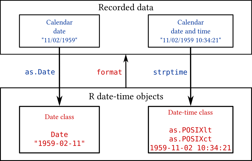
FIGURE 4.3: Displayed are functions to convert calendar date and time data into R date-time classes (as.Date, strptime, as.POSIXlt, as.POSIXct), and the format function converts date-time objects into character dates, days, weeks, months, times, etc.
4.9.1 Date functions in the base package
4.9.1.1 The as.Date function
Let’s start with simple date calculations. The as.Date
function in R converts calendar dates (e.g., 11/2/1949) into a
Date objects—a numeric vector of class Date. The
numeric information is the number of days since January 1, 1970—also
called Julian dates. However, because calendar date data can come in a
variety of formats, we need to specify the format so that
as.Date does the correct conversion. Study the following
analysis carefully.
#> [1] "11/2/1959" "1/1/1970"#### convert to Julian dates
bdays.julian <- as.Date(bdays, format = "%m/%d/%Y")
bdays.julian # numeric vector of class data#> [1] "1959-11-02" "1970-01-01"#> [1] -3713 0#> [1] "2019-12-22"#> Time differences in days
#> [1] 60.13689 49.97125#### the display of 'days' is not correct
#### truncate number to get "age"
age2 <- trunc(as.numeric(age))
age2#> [1] 60 49#### create date frame
bd <- data.frame(Birthday = bdays, Standard = bdays.julian,
Julian = as.numeric(bdays.julian), Age = age2)
bd#> Birthday Standard Julian Age
#> 1 11/2/1959 1959-11-02 -3713 60
#> 2 1/1/1970 1970-01-01 0 49Notice that although bdays.julian appears like a character vector,
it is actually a numeric vector of class date. Use the class and
mode functions to verify this.
To summarize, as.Date converted the character vector of calendar
dates into Julian dates (days since 1970-01-01) are displayed in a
standard format (yyyy-mm-dd). The Julian dates can be used in
numerical calculations. To see the Julian dates use as.numeric or
julian function. Because the calendar dates to be converted can come
in a diversity of formats (e.g., November 2, 1959; 11-02-59;
11-02-1959; 02Nov59), one must specify the format option in
as.Date. Below are selected format options; for a complete list see
help(strptime).
| Abbrev. | Description |
|---|---|
%a |
Abbreviated weekday name. |
%A |
Full weekday name. |
%b |
Abbreviated month name. |
%B |
Full month name. |
%d |
Day of the month as decimal number (01-31) |
%j |
Day of year as decimal number (001-366). |
%m |
Month as decimal number (01-12). |
%U |
Week of the year as decimal number (00-53) using the first Sunday as day 1 of week 1. |
%w |
Weekday as decimal number (0-6, Sunday is 0). |
%W |
Week of the year as decimal number (00-53) using the first Monday as day 1 of week 1. |
%y |
Year without century (00-99). Century you get is system-specific. So don’t!. |
%Y |
Year with century. |
Here are some examples of converting dates with different formats:
#> [1] "1959-11-02"#> [1] "1959-11-02"#> [1] "2059-11-02"#> [1] "1959-11-02"#> [1] "2059-11-02"#> [1] "1959-11-02"Notice how Julian dates can be used like any integer:
#> [1] 12432 12433 12434 12435 12436 12437 12438 12439 12440#> [1] "2004-01-15" "2004-01-16" "2004-01-17" "2004-01-18"4.9.1.2 The weekdays, months, quarters, julian functions
Use the weekdays, months, quarters, or julian functions to
extract information from Date and other date-time objects in R.
#> [1] "Thursday" "Thursday" "Friday"#> [1] "January" "April" "October"#> [1] "Q1" "Q2" "Q4"#> [1] 12432 12523 12706
#> attr(,"origin")
#> [1] "1970-01-01"4.9.1.3 The strptime function
So far we have worked with calendar dates; however, we also need to be
able to work with times of the day. Whereas as.Date only
works with calendar dates, the strptime function will accept
data in the form of calendar dates and times of the day (HH:MM:SS,
where H = hour, M = minutes, S = seconds). For example, let’s look at
the Oswego foodborne ill outbreak that occurred in 1940. The source of
the outbreak was attributed to the church supper that was served on
April 18, 1940. The food was available for consumption from 6 pm to 11
pm. The onset of symptoms occurred on April 18th and 19th. The meal
consumption times and the illness onset times were recorded.
#> 'data.frame':    75 obs. of  21 variables:
#>  $ id            : int  2 3 4 6 7 8 9 10 14 16 ...
#>  $ age           : int  52 65 59 63 70 40 15 33 10 32 ...
#>  $ sex           : chr  "F" "M" "F" "F" ...
#>  $ meal.time     : chr  "8:00 PM" "6:30 PM" "6:30 PM" "7:30 PM" ...
#>  $ ill           : chr  "Y" "Y" "Y" "Y" ...
#>  $ onset.date    : chr  "4/19" "4/19" "4/19" "4/18" ...
#>  $ onset.time    : chr  "12:30 AM" "12:30 AM" "12:30 AM" "10:30 PM" ...
#>  $ baked.ham     : chr  "Y" "Y" "Y" "Y" ...
#>  $ spinach       : chr  "Y" "Y" "Y" "Y" ...
#>  $ mashed.potato : chr  "Y" "Y" "N" "N" ...
#>  $ cabbage.salad : chr  "N" "Y" "N" "Y" ...
#>  $ jello         : chr  "N" "N" "N" "Y" ...
#>  $ rolls         : chr  "Y" "N" "N" "N" ...
#>  $ brown.bread   : chr  "N" "N" "N" "N" ...
#>  $ milk          : chr  "N" "N" "N" "N" ...
#>  $ coffee        : chr  "Y" "Y" "Y" "N" ...
#>  $ water         : chr  "N" "N" "N" "Y" ...
#>  $ cakes         : chr  "N" "N" "Y" "N" ...
#>  $ van.ice.cream : chr  "Y" "Y" "Y" "Y" ...
#>  $ choc.ice.cream: chr  "N" "Y" "Y" "N" ...
#>  $ fruit.salad   : chr  "N" "N" "N" "N" ...
To calculate the incubation period, for ill individuals, we need to subtract the meal consumption times (occurring on 4/18) from the illness onset times (occurring on 4/18 and 4/19). Therefore, we need two date-time objects to do this arithmetic. First, let’s create a date-time object for the meal times:
#> [1] "8:00 PM" "6:30 PM" "6:30 PM" "7:30 PM" "7:30 PM"#### create character vector with meal date and time
mdt <- paste("4/18/1940", odat$meal.time)
mdt[1:4]#> [1] "4/18/1940 8:00 PM" "4/18/1940 6:30 PM" "4/18/1940 6:30 PM"
#> [4] "4/18/1940 7:30 PM"#### convert into standard date and time
meal.dt <- strptime(mdt, format = "%m/%d/%Y %I:%M %p")
meal.dt[1:4]#> [1] "1940-04-18 20:00:00 PST" "1940-04-18 18:30:00 PST"
#> [3] "1940-04-18 18:30:00 PST" "1940-04-18 19:30:00 PST"#> [1] "4/19" "4/19" "4/19" "4/18"#> [1] "12:30 AM" "12:30 AM" "12:30 AM" "10:30 PM"#### create vector with onset date and time
odt <- paste(paste(odat$onset.date, "/1940", sep=""),
odat$onset.time)
odt[1:4]#> [1] "4/19/1940 12:30 AM" "4/19/1940 12:30 AM"
#> [3] "4/19/1940 12:30 AM" "4/18/1940 10:30 PM"#### convert into standard date and time
onset.dt <- strptime(odt, "%m/%d/%Y %I:%M %p")
onset.dt[1:4]#> [1] "1940-04-19 00:30:00 PST" "1940-04-19 00:30:00 PST"
#> [3] "1940-04-19 00:30:00 PST" "1940-04-18 22:30:00 PST"#> Time differences in hours
#> [1] 4.5 6.0 6.0 3.0 3.0 6.5 3.0 4.0 6.5 NA NA NA NA 3.0 NA
#> [16] NA NA 3.0 NA NA 3.0 3.0 NA NA 3.0 NA NA NA NA NA
#> [31] 6.0 NA 4.0 NA NA NA 3.0 7.0 4.0 3.0 NA NA 5.5 4.5 NA
#> [46] NA NA NA NA NA NA NA NA NA NA NA NA NA NA NA
#> [61] NA NA NA NA NA NA NA NA NA NA NA NA NA NA NA#> Time difference of 4.295455 hours#> Time difference of 4 hours#> [1] 4To summarize, we used strptime to convert the meal
consumption date and times and illness onset dates and times into
date-time objects (meal.dt and onset.dt) that can be
used to calculate the incubation periods by simple subtraction (and
assigned name incub.period).
Notice that incub.period is an atomic object of class
difftime:
#>  'difftime' num [1:75] 4.5 6 6 3 ...
#>  - attr(*, "units")= chr "hours"
This is why we had trouble calculating the median (which should not be
the case). We got around this problem by coercion using
as.numeric:
#> [1] NANow, what kind of objects were created by the strptime
function?
#> POSIXlt[1:75], format: "1940-04-18 20:00:00" "1940-04-18 18:30:00" ...#> POSIXlt[1:75], format: "1940-04-19 00:30:00" "1940-04-19 00:30:00" ...The strptime function produces a named list of class
POSIXlt. POSIX stands for Portable Operating System Interface,'' andlt’’ stands for “legible
time.”28
4.9.1.4 The POSIXlt and POSIXct functions
The POSIXlt list contains the date-time data in human readable forms. The named list contains the following vectors:
| Names | Values: description |
|---|---|
| ‘sec’ | 0-61: seconds |
| ‘min’ | 0-59: minutes |
| ‘hour’ | 0-23: hours |
| ‘mday’ | 1-31: day of the month |
| ‘mon’ | 0-11: months after the first of the year. |
| ‘year’ | Years since 1900. |
| ‘wday’ | 0-6 day of the week, starting on Sunday. |
| ‘yday’ | 0-365: day of the year. |
| ‘isdst’ | Daylight savings time flag. Positive if in force, zero if not, negative if unknown. |
Let’s examine the onset.dt object we created from the Oswego data.
#> [1] TRUE#> NULL#> [1] 30#> [1] 10#> [1] 19#> [1] 3#> [1] 40#> [1] 5#> [1] 109The POSIXlt list contains useful date-time information; however, it is
not in a convenient form for storing in a data frame. Using as.POSIXct
we can convert it to a `continuous time'' object that contains the number of seconds since 1970-01-01 00:00:00.as.POSIXlt` coerces a
date-time object to POSIXlt.
#> [1] "1940-04-19 10:30:00 PST" NA
#> [3] NA                        NA
#> [5] NA#> [1] -937287000 NA NA NA NA4.9.1.5 The format function
Whereas the strptime function converts a character vector of
date-time information into a date-time object, the format
function converts a date-time object into a character vector. The
format function gives us great flexibility in converting
date-time objects into numerous outputs (e.g., day of the week, week
of the year, day of the year, month of the year, year). Selected
date-time format options are listed on TODO-REF, for a complete list see
help(strptime).
For example, in public health, reportable communicable diseases are
often reported by “disease week” (this could be week of reporting or
week of symptom onset). This information is easily extracted from R
date-time objects. For weeks starting on Sunday use the %U option
in the format function, and for weeks starting on Monday use the
%W option.
#>  [1] "2003-12-15" "2003-12-16" "2003-12-17" "2003-12-18"
#>  [5] "2003-12-19" "2003-12-20" "2003-12-21" "2003-12-22"
#>  [9] "2003-12-23" "2003-12-24" "2003-12-25" "2003-12-26"
#> [13] "2003-12-27" "2003-12-28" "2003-12-29" "2003-12-30"
#> [17] "2003-12-31" "2004-01-01" "2004-01-02" "2004-01-03"
#> [21] "2004-01-04" "2004-01-05" "2004-01-06" "2004-01-07"
#> [25] "2004-01-08" "2004-01-09" "2004-01-10" "2004-01-11"
#> [29] "2004-01-12" "2004-01-13" "2004-01-14" "2004-01-15"#> [1] "50" "50" "50" "50" "50" "50" "51" "51" "51" "51" "51" "51"
#> [13] "51" "52" "52" "52" "52" "00" "00" "00" "01" "01" "01" "01"
#> [25] "01" "01" "01" "02" "02" "02" "02" "02"4.9.2 Date functions in the chron and survival packages
The chron and survival packages have customized functions for
dealing with dates. Both packages come with the default R
installation. To learn more about date and time classes read R News,
Volume 4/1, June 2004.29
4.10 Exporting data objects
| Function and description | Try these examples |
|---|---|
| Export to Generic ASCII text file | |
| write.table | |
| Write tabular data as a data frame to an ASCII text file. | write.table(infert,"infert.txt") |
Read file back in using read.table function |
|
| write.csv | |
| Write tabular data as a data frame to an ASCII text .csv file. | write.csv(infert,"infert.csv") |
Read file back in using read.csv function |
|
| write | |
| Write matrix elements to an ASCII text file | x <- matrix(1:4, 2, 2) |
write(t(x), "x.txt") |
|
| Export to R ASCII text file | |
| dump | |
| “Dumps” list of R objects as R code to an ASCII text file; | dump("Titanic", "titanic.R") |
Read back in using source function |
|
| dput | |
| Writes an R object as R code to the console, or an ASCII text file. | dput(Titanic, "titanic.R") |
Read file back in using dget function |
|
| Export to R binary file | |
| save | |
“Saves” list of R objects as binary filename .Rdata file. |
save(Titanic, "titanic.Rdata") |
Read back in using load function. |
|
| Export to non-R ASCII text file | |
| write.foreign | |
From foreign package: writes non-R text files (SPSS, Stata, SAS). |
write.foreign(infert, datafile="infert.dat", |
Use foreign package to read in |
codefile="infert.txt", package = "SPSS") |
| Export to non-R binary file | |
| write.dbf | |
From foreign package: writes DBF files |
write.dbf(infert, "infert.dbf") |
| write.dta | |
From foreign package: writes files in Stata binary format |
write.dta(infert, "infert.dta") |
On occassion, we need to export R data objects. This can be done in several ways, depending on our needs: - Generic ASCII text file - R ASCII text file - R binary file - Non-R ASCII text files - Non-R binary file
4.10.1 Exporting to a generic ASCII text file
4.10.1.1 The write.table function
We use the write.table function to exports a data frame as a
tabular ASCII text file which can be read by most statistical
packages. If the object is not a data frame, it converts to a data
frame before exporting it. Therefore, this function only make sense
with tabular data objects. Here are the default arguments:
#> function (x, file = "", append = FALSE, quote = TRUE, sep = " ",
#>     eol = "\n", na = "NA", dec = ".", row.names = TRUE, col.names = TRUE,
#>     qmethod = c("escape", "double"), fileEncoding = "")
#> NULL
The 1st argument will be the data frame name (e.g., infert), the 2nd
will be the name for the output file (e.g., infert.dat), the
sep argument is set to be space-delimited, and the
row.names argument is set to TRUE.
The following code:
produces this ASCII text file:
"education" "age" "parity" "induced" "case" ...
"1" "0-5yrs" 26 6 1 1 2 1 3
"2" "0-5yrs" 42 1 1 1 0 2 1
"3" "0-5yrs" 39 6 2 1 0 3 4
"4" "0-5yrs" 34 4 2 1 0 4 2
"5" "6-11yrs" 35 3 1 1 1 5 32
...
Because row.names=TRUE, the number field names in the header
(row 1) will one less that the number of columns (starting with row
2). The default row names is a character vector of integers. The
following code:
produces a commna-delimited ASCII text file without row names:
"education","age","parity","induced","case", ...
"0-5yrs",26,6,1,1,2,1,3
"0-5yrs",42,1,1,1,0,2,1
"0-5yrs",39,6,2,1,0,3,4
"0-5yrs",34,4,2,1,0,4,2
"6-11yrs",35,3,1,1,1,5,32
...
Note that the write.csv function produces a comma-delimited
data file by default.
4.10.1.2 The write function
The write function writes the contents of a matrix in a
columnwise order to an ASCII text file. To get the same appearance as
the matrix, we must transpose the matrix and specify the number of
columns (the default is 5). If we set file="", then the
output is written to the screen:
#>     parity
#> case  1  2  3  4  5  6
#>    0 66 54 24 12  4  5
#> 1 33 27 12 6 2 3#> 66 33 54 27 24
#> 12 12 6 4 2
#> 5 3#> 66 54 24 12 4 5
#> 33 27 12 6 2 3To read the raw data back into R, we would use the scan
function. For example, if the data had been written to
data.txt, then the following code reads the data back into R:
matrix(scan("data.txt"), ncol=6, byrow=TRUE)
#> Read 12 items
#>      [,1] [,2] [,3] [,4] [,5] [,6]
#> [1,]   66   54   24   12    4    5
#> [2,]   33   27   12    6    2    3
Of course, all the labeling was lost.
4.10.2 Exporting to R ASCII text file
Data objects can also be exported as R code in an ASCII text file
using the dump and dput functions. This has
advantages for complex R objects (e.g., arrays, lists) that do not
have simple tabular structures, and the R code makes the raw data
human legible.
4.10.2.1 The dump function
The dump function exports multiple objects as R code as the
next example illustrates:
infert.tab1 <- xtabs(~case+parity,data=infert)
infert.tab2 <- xtabs(~education+parity+case,data=infert)
infert.tab1 #display matrix
#> parity
#> case 1 2 3 4 5 6
#> 0 66 54 24 12 4 5
#> 1 33 27 12 6 2 3#> , , case = 0
#>
#> parity
#> education 1 2 3 4 5 6
#> 0-5yrs 2 0 0 2 0 4
#> 6-11yrs 28 28 14 8 2 0
#> 12+ yrs 36 26 10 2 2 1
#>
#> , , case = 1
#>
#> parity
#> education 1 2 3 4 5 6
#> 0-5yrs 1 0 0 1 0 2
#> 6-11yrs 14 14 7 4 1 0
#> 12+ yrs 18 13 5 1 1 1The dump function produced the following R code in the
infert_tab.R text file:
`infert.tab1` <-
structure(c(66, 33, 54, 27, 24, 12, 12, 6, 4, 2, 5, 3),
.Dim = c(2L, 6L), .Dimnames = structure(list(case = c("0", "1"),
parity = c("1", "2", "3", "4", "5", "6")), .Names = c("case",
"parity")), class = c("xtabs", "table"), call = quote(xtabs(
formula = ~case + parity, data = infert)))
`infert.tab2` <-
structure(c(2, 28, 36, 0, 28, 26, 0, 14, 10, 2, 8, 2, 0, 2,
2, 4, 0, 1, 1, 14, 18, 0, 14, 13, 0, 7, 5, 1, 4, 1, 0, 1, 1,
2, 0, 1), .Dim = c(3L, 6L, 2L), .Dimnames = structure(list(
education = c("0-5yrs", "6-11yrs", "12+ yrs"), parity = c("1",
"2", "3", "4", "5", "6"), case = c("0", "1")), .Names =
c("education", "parity", "case")), class = c("xtabs", "table"),
call = quote(xtabs(formula = ~education + parity + case,
data = infert)))Notice that the 1st argument was a character vector of object names.
The infert_tab.R file can be run in R using the
source function to recreate all the objects in the workspace.
4.10.2.2 The dput function
The dput function is similar to the dump function
except that the object name is not written. By default, the
dput function prints to the screen:
#> structure(c(66L, 33L, 54L, 27L, 24L, 12L, 12L, 6L, 4L, 2L, 5L,
#> 3L), .Dim = c(2L, 6L), .Dimnames = list(case = c("0", "1"), parity = c("1",
#> "2", "3", "4", "5", "6")), class = c("xtabs", "table"), call = xtabs(formula = ~case +
#> parity, data = infert))To export to an ASCII text file, give a new file name as the second
argument, similar to dump. To get back the R code use the dget
function:
#>     parity
#> case  1  2  3  4  5  6
#>    0 66 54 24 12  4  5
#> 1 33 27 12 6 2 34.10.3 Exporting to R binary file
4.10.3.1 The save function
The save function exports R data objects to binary file
(filename.RData) which is the most effient, compact
method to export objects. The first argument(s) can be the names of
the objects to save followed by the output file name, or list with a
character vector of object names followed by the output file
name. Here is an example of the first option:
x <- 1:5; y <- x^3
save(x, y, file="~/git/phds/example/xy.RData")
rm(x, y)
load(file="~/git/phds/example/xy.RData")
x; y#> [1] 1 2 3 4 5#> [1] 1 8 27 64 125Notice that we used the load function to load the binary file
back into the workspace.
Now here is an example of the second option using a list:
x <- 1:5; y <- x^3
save(list=c("x", "y"), file="~/git/phds/example/xy.RData")
rm(x, y)
load(file="~/git/phds/example/xy.RData")
x; y#> [1] 1 2 3 4 5#> [1] 1 8 27 64 125In fact, the save.image function we use to save the entire
workspace is just the following:
4.10.4 Exporting to non-R ASCII text and binary files
The foreign package contains functions for exporting R data
frames to non-R ASCII text and binary files. The
write.foreign function write two ASCII text files: the first
file is the data file, and the second file is the code file for
reading the data file. The code file contains either SPSS, Stata, or
SAS programming code. The write.dbf function writes a data
frame to a binary DBF file, which can be read back into R using the
read.dbf function. Finally, the write.dta function
writes a data frame to a binary Stata file, which can be read back
into R using the read.dta function.
4.11 Working with regular expressions
A regular expression is a special text string for describing a search pattern which can be used for searching text strings, indexing data objects, and replacing object elements. For example, we applied Global Burden of Disease methods to evaluate causes of premature deaths in San Francisco [16]. Using regular expressions we were able to efficiently code over 14,000 death records, with over 900 ICD-10 cause of death codes, into 117 mutually exclusive cause of death categories. Without regular expressions, this local area study would have been prohibitively tedious.
A regular expression is built up from specifying one character at a time. Using this approach, we cover the following:
- Single character: matching a single character;
- Character class: matching a single character from among a list of characters;
- Concatenation: combining single characters into a new match pattern;
- Repetition: specifying how many times a single character or match pattern might be repeated;
- Alternation: a regular expression may be matched from among two or more regular expressions; and
- Metacharacters: special characters that require special treatment.
4.11.1 Single characters
The search pattern is built up from specifying one character at a
time. For example, the pattern "x" looks for the letter
x in a text string. Next, consider a character vector of
text strings. We can use the grep function to search for a
pattern in this data vector.
vec1 <- c("x", "xa bc", "abc", "ax bc", "ab xc", "ab cx",
"z rox z", "y xo y", "xy aba", "cba")
grep("x", vec1)#> [1] 1 2 4 5 6 7 8 9#> [1] "x" "xa bc" "ax bc" "ab xc" "ab cx" "z rox z"
#> [7] "y xo y" "xy aba"#> [1] "x" "xa bc" "ax bc" "ab xc" "ab cx" "z rox z"
#> [7] "y xo y" "xy aba"The grep function returned an integer vector indicating the
positions in the data vector that contain a match. We used this
integer vector to index by position.
We distinguish between matching a pattern at the beginning or end of a
line versus matching a pattern at the beginning or end of a word. The
caret ^ matches the empty string at the beginning of a
line. Therefore, to match this pattern at the beginning of a line we
add the ^ character to the regular expression:
#> [1] "x" "xa bc" "xy aba"The $ character matches the empty string at the end of a
line. Therefore, to match this pattern at the end of a line we add the
$ character to the regular expression:
#> [1] "x" "ab cx"The ^ and $ characters are examples of metacharacters which have
special meanings in regular expression functions. We learn more about
metacharacter later.
The symbol \b matches the empty string at the edge of a word, and
\B matches the empty string provided it is not at the edge of a
word. The backslash \ is a special character; therefore, to use
\b in a matching pattern we need to add an escape backslash (\) to
\b; in other words use \\b. Study these examples:
#> [1] "x" "xa bc" "ab xc" "y xo y" "xy aba"#> [1] "x" "ax bc" "ab cx" "z rox z"#> [1] "x"#> [1] "ax bc" "ab cx" "z rox z"#> [1] "xa bc" "ab xc" "y xo y" "xy aba"#> character(0)The symbol \< matches the pattern at the beginning of the word, and
\> matches the pattern at the end of the word. For practical
purposes, \b and either \< or \> will yield the same results.
The period (.) matches any single character, including a space.
#> [1] "xa bc" "abc" "ax bc"In this example the . was followed by two characters bc. Appending
characters is called concatenation and is covered later in detail.
| Regular expression | Description | Example |
|---|---|---|
. |
Any single character | "a.c" |
^ |
At beginning of line | "^F" |
$ |
At end of line | "F$" |
\b |
At edge of a word | "\\bF", "F\\b" |
\B |
Not at edge of a word | "\\BF", "F\\B" |
\< |
Beginning of a word | "\\<F" |
\> |
End of a word | "F\\>" |
4.11.2 Character class
A character class is a list of characters enclosed by square
brackets [ and ] which matches any single character in that
list. For example, "[fhr]" will match the single character f, h,
or r. This can be combined with metacharacters for more specificity;
for example, "^[fhr]" will match the single character f, h, or
r at the beginning of a line.
#> [1] "fat" "rat" "hat"As already shown, ^ character matches the empty string at the
beginning of a line. However, when ^ is the first character in a
character class list, it matches any character not in the list. For
example, "^[^fhr]" will match any single character at the beginning
of a line except f, h, or r.
#> [1] "bar" "elf" "mach"Character classes can be specified as a range of possible
characters. For example, [0-9] matches a single digit with possible
values from 0 to 9, [A-Z] matches a single letter with possible
values from A to Z, and [a-z] matches a single letter from a
to z. The pattern [0-9A-Za-z] matches any single alphanumeric
character. Table 4.8 displays additional selected
character class regular expessions.
| Regular expression | Description | Alternative |
|---|---|---|
\d |
Digits | [0-9] |
\D |
Non-digits | [^0-9] |
\w |
Word character | [A-Za-z0-9_] |
\W |
Not work character | [^A-Za-z0-9_] |
\s |
Space | |
\S |
Non-space |
#> [1] "hello" "1234" "_"#> [1] "?" " " "\n" "&"For convenience, certain character classes are predefined and their
interpretation depend on
locale.30
For example, to match a single lower case letter we place [:lower:]
inside square brackets like this: "[[:lower:]]", which is equivalent
to "[a-z]". Table 4.9 lists predefined character
classes. This is very convenient for matching punctuation characters
and multiple types of spaces (e.g., tab, newline, carriage
return). The [:punct:] character class matches any of the following
punctuation characters:
! " # $ % & ' ( ) * + , - . / : ; < = > ? @ [ \ ] ^ _ ` { | } ~| Predefined | Description | Alternative |
|---|---|---|
| [[:lower:]] | Lower-case letters | [a-z] |
| [[:upper:]] | Upper-case letters | [A-Z] |
| [[:alpha:]] | Alphabetic characters | [A-Za-z] or [[:lower:][:upper:]] |
| [[:digit:]] | Digits | [0-9] |
| [[:alnum:]] | Alphanumeric characters | [A-Za-z0-9] or [[:alpha:][:digit:]] |
| [[:punct:]] | Punctuation characters: | |
| [[:blank:]] | Blank characters31 | |
| [[:cntrl:]] | Control characters32 | |
| [[:space:]] | Space characters33 | |
| [[:graph:]] | Graphical characters | [[:alnum:][:punct:]] |
| [[:print:]] | Printable characters | [[:alnum:][:punct:][:space:]] |
| [[:xdigit:]] | Hexadecimal digits: | [0-9A-Fa-f] |
In this final example, "^.[^a].+" will match any first
character, followed by any character except a, and followed
by any character one or more times:
#> [1] "elf"Combining single character matches is call concatenation and is covered next.
4.11.3 Concatenation
Single characters (including character classes) can be
concatenated; for example, the pattern "ˆ[fhr]at$"
will match the single, isolated words fat, hat, or
rat.
vec3 <- c("fat", "bar", "rat", "fat boy", "elf", "mach", "hat")
grep("^[fhr]at$", vec3, value = TRUE)#> [1] "fat" "rat" "hat"The concatenation "[ct]a[br]" will match the pattern that
starts with c or t, followed by a, and
followed by b or r.
vec4 <- c("cab", "carat", "tar", "bar", "tab", "batboy", "care")
grep("[ct]a[br]", vec4, value = TRUE)#> [1] "cab" "carat" "tar" "tab" "care"To match single, 3-letter words use "\\b[ct]a[br]\\b".
#> [1] "cab" "tar" "tab"The period (.) is another metacharacter: it matches any
single character. For example, "f.t" matches the pattern
f + any character + t.
#> [1] "fate" "fit" "futbol"4.11.4 Repetition
| Repetition quantifier | Description |
|---|---|
? |
Preceding pattern is optional and will be matched at most once |
* |
Preceding pattern will be matched zero or more times |
+ |
Preceding pattern will be matched one or more times |
{n} |
Preceding pattern is matched exactly n times |
{n,} |
Preceding pattern is matched n or more times |
{n, m} |
Preceding pattern is matched at least n times, but not more than m times |
Regular expressions (so far: single characters, character classes, and
concatenations) can be qualified by whether a pattern can repeat
(Table 4.10). For example, the pattern "^[fF].+t$"
matches single, isolated words that start with f or F, followed by
1 or more of any character, and ending with t.
vec6 <- c("fat", "fate", "feat", "bat", "Fahrenheit", "bat", "foot")
grep("^[fF].+t$", vec6, value = TRUE)#> [1] "fat" "feat" "Fahrenheit" "foot"Repetition quantifiers gives us great flexibility to specify how often preceding patterns can repeat.
4.11.5 Alternation
Two or more regular expressions (so far: single characters, character
classes, concatenations, and repetitions) may be joined by the infix
operator |. The resulting regular expression can match the
pattern of any subexpression. For example, the World Health
Organization (WHO) Global Burden of Disease (GBD) Study used
International Classification of Diseases, 10th Revision (ICD-10) codes
(ref). The GBD Study ICD-10 codes for hepatitis B are the following:
B16, B16.0, B16.1, B16.2, B16.3, B16.4, B16.5, B16.7, B16.8,
B16.9, B17, B17.0, B17.2, B17.8, B18, B18.0, B18.1, B18.8, B18.9Notice that B16 and B16.0 are not the same ICD-10 code! The GBD Study methods were used to study causes of death in San Francisco, California (ref). Underlying causes of death were obtained from the State of California, Center for Health Statistics. The ICD-10 code field did not have periods so that the hepatitis B codes were the following.
B16, B160, B161, B162, B163, B164, B165, B167, B168, B169, B17,
B170, B172, B178, B18, B180, B181, B188, B189To match the pattern of ICD-10 codes representing hepatitis B, the following regular expression was used (without spaces):
"^B16[0-9]?$|^B17[0,2,8]?$|^B18[0,1,8,9]?$"This regular expression matches ˆB16[0-9]?$ or ˆB17[0,2,8]?$ or
ˆB18[0,1,8,9]?$. Similar to the first and third pattern, the second
regular expression, ˆB17[0,2,8]?$, matches B17, B170, B172, or
B178 as isolated text strings.
To see how this works, we can match each subexpression individually and then as an alternation:
hepb <- c("B16", "B160", "B161", "B162", "B163", "B164", "B165",
"B167", "B168", "B169", "B17", "B170", "B172", "B178",
"B18", "B180", "B181", "B188", "B189")
grep("^B16[0-9]?$", hepb, value = TRUE) # match 1st subexpression#> [1] "B16" "B160" "B161" "B162" "B163" "B164" "B165" "B167"
#> [9] "B168" "B169"#> [1] "B17" "B170" "B172" "B178"#> [1] "B18" "B180" "B181" "B188" "B189"#> [1] "B16" "B160" "B161" "B162" "B163" "B164" "B165" "B167"
#> [9] "B168" "B169" "B17" "B170" "B172" "B178" "B18" "B180"
#> [17] "B181" "B188" "B189"A natural use for these pattern matches is for indexing and replacement. We illustrate this using the 2nd subexpression.
#> [1] "B17" "B170" "B172" "B178"#> [1] "B16" "B160" "B161" "B162" "B163" "B164" "B165" "B167"
#> [9] "B168" "B169" "HBV" "HBV" "HBV" "HBV" "B18" "B180"
#> [17] "B181" "B188" "B189"Using regular expression alternations allowed us to efficiently code
over 14,000 death records, with over 900 ICD-10 cause of death codes,
into 117 mutually exclusive cause of death categories for our San
Francisco study. Suppose sfdat was the data frame with San
Francisco deaths for 2003–2004. Then the following code would
tabulate the deaths caused by hepatatis B:
sfdat$hepb <- rep("No", nrow(sfdat)) #new field
get.hepb <- grep("^B16[0-9]?$|^B17[0,2,8]?$|^B18[0,1,8,9]?$",
sfdat$icd10)
sfdat$hepb[get.hepb] <- "Yes"
table(sfdat$hepb)Therefore, in San Francisco, during the period 2003-2004, there were 23 deaths caused by hepatitis B. Without regular expressions, this mortality analysis would have been prohibitively tedious.
In this next example we use regular expressions to correct misspelled data. Suppose we have a data vector containing my first name (“Tomas”), but sometimes misspelled. We want to locate the most common misspellings and correct them:
tdat <- c("Tom", "Thomas", "Tomas", "Tommy", "tomas")
misspelled <- grep("^[Tt]omm?y?$|^[Tt]homas$|^tomas$", tdat)
misspelled#> [1] 1 2 4 5#> [1] "Tomas" "Tomas" "Tomas" "Tomas" "Tomas"4.11.6 Repetition > Concatenation > Alternation
Repetition takes precedence over concatenation, which in turn takes precedence over alternation. A whole subexpression may be enclosed in parentheses to override these precedence rules. For example, consider how the following regular expression changes when parentheses are used give concatenation precedence over repetition:
vec7 <- c("Tommy", "Tomas", "Tomtom")
grep("[Tt]om{2,}", vec7, value=TRUE) # repetition takes precedence#> [1] "Tommy"#> [1] "Tomtom"Recall that {2,} means repeat the previous 2 or more times.
4.11.7 Metacharacters
| Char. | Description | Example | Literal search |
|---|---|---|---|
^ |
Matches empty string at beginning of line | "^my car" |
See p. TODO |
| When 1st character in character class, matches any single character not in the list | "[^abc]" |
See p. TODO | |
$ |
Matches empty string at end of line | "my car$" |
"[$]" |
[ |
Character class | "[[]" |
|
. |
Matches any single character | "p.t" |
"[.]" |
? |
Repetition quantifier (Table 4.10) | ".?" |
"[?]" |
* |
Repetition quantifier (Table 4.10) | ".*" |
"[*]" |
+ |
Repetition quantifier (Table 4.10) | ".+" |
"[+]" |
( ) |
Grouping subexpressions | "([Tt]om){2,}" |
"[(]" or "[)]" |
| \(\mid\) | Join subexpresions, any of which can be matched | "Tomas\(\mid\)Luis" |
"[\(\mid\)]" |
RStudio provides a very useful Cheat Sheet for basic regular expressions here: https://rstudio.com/wp-content/uploads/2016/09/RegExCheatsheet.pdf.
4.12 Exercises
See Appendix C for description of data sets and data dictionary.
#### (1)
edat <- read.table("~/data/evans.txt", header = TRUE, sep = "")
str(edat)
xtabs(~chd, data = edat)
edat$chd2 <- factor(edat$chd, levels = 0:1,
labels = c("No", "Yes"))
xtabs(~chd2, data = edat) # test
xtabs(~cat, data = edat)
edat$cat2 <- factor(edat$cat, levels = 0:1,
labels = c("Normal", "High"))
xtabs(~cat2, data = edat) # test
xtabs(~smk, data = edat)
edat$smk2 <- factor(edat$smk, levels = 0:1,
labels = c("Never", "Ever"))
xtabs(~smk2, data = edat) # test
xtabs(~ecg, data = edat)
edat$ecg2 <- factor(edat$ecg, levels = 0:1,
labels = c("Normal", "Abnormal"))
xtabs(~ecg2, data = edat) # test
xtabs(~hpt, data = edat)
edat$hpt2 <- factor(edat$hpt, levels = 0:1,
labels = c("No", "Yes"))
xtabs(~hpt2, data = edat) # test
#### (2)
quantile(edat$age)
edat$age4 <- cut(edat$age, quantile(edat$age), right = FALSE,
include.lowest = TRUE)
xtabs(~age4, data = edat) # test
#### (3)
hptnew <- rep(NA, nrow(edat))
normal <- edat$sbp < 120 & edat$dbp < 80
hptnew[normal] <- 1
prehyp <- (edat$sbp >= 120 & edat$sbp < 140) |
(edat$dbp >= 80 & edat$dbp < 90)
hptnew[prehyp] <- 2
stage1 <- (edat$sbp >= 140 & edat$sbp < 160) |
(edat$dbp >= 90 & edat$dbp < 100)
hptnew[stage1] <- 3
stage2 <- edat$sbp >= 160 | edat$dbp >= 100
hptnew[stage2] <- 4
edat$hpt4 <- factor(hptnew, levels = 1:4,
labels=c("Normal", "PreHTN", "HTN.Stage1",
"HTN.Stage2"))
xtabs(~hpt4, data = edat) # test
#### (4)
xtabs(~hpt2 + hpt4, data = edat)~/data/wnv/wnv2004raw.csv. Read in the
data setting as.is = TRUE, taking into account missing values (use
na.strings option). Convert the calendar dates into the
international standard format. Using the write.table function
export the data as an ASCII text file.
Hint provided:
wdat <- read.table("~/data/wnv/wnv2004raw.csv", header = TRUE,
sep = ",", as.is = TRUE, na.strings = c(".","Unknown"))
str(wdat)
wdat$date.onset2 <- as.Date(wdat$date.onset, format = "%m/%d/%Y")
wdat$date.tested2 <- as.Date(wdat$date.tested, format = "%m/%d/%Y")
write.table(wdat, "~/git/phds/example/wnvdat.txt",
sep = ",", row.names = FALSE)
wdat.test <- read.csv("~/git/phds/example/wnvdat.txt")
head(wdat.test)
str(wdat.test)See Appendix C for data dictionary.
When Dr. Rubin arrived in the field, he learned from the health officer that all persons known to be ill had attended a church supper held on the previous evening, April 18. Family members who did not attend the church supper did not become ill. Accordingly, Dr. Rubin focused the investigation on the supper. He completed Interviews with 75 of the 80 persons known to have attended, collecting information about the occurrence and time of onset of symptoms, and foods consumed. Of the 75 persons interviewed, 46 persons reported gastrointestinal illness.
The onset of illness in all cases was acute, characterized chiefly by nausea, vomiting, diarrhea, and abdominal pain. None of the ill persons reported having an elevated temperature; all recovered within 24 to 30 hours. Approximately 20% of the ill persons visited physicians. No fecal specimens were obtained for bacteriologic examination. The investigators suspected that this was a vehicle-borne outbreak, with food as the vehicle. Dr. Rubin put his data into a line listing. See the raw data set at ~/data/oswego/oswego.txt.
The supper was held in the basement of the village church. Foods were contributed by numerous members of the congregation. The supper began at 6:00 p.m. and continued until 11:00 p.m. Food was spread out on a table and consumed over a period of several hours. Data regarding onset of illness and food eaten or water drunk by each of the 75 persons interviewed are provided in the line listing. The approximate time of eating supper was collected for only about half the persons who had gastrointestinal illness.
- Using RStudio plot the cases by time of onset of illness (include
appropriate labels and title). What does this graph tell you?
(Hint: Process the text data and then use the
histfunction.) - Are there any cases for which the times of onset are inconsistent with the general experience? How might they be explained?
- How could the data be sorted by illness status and illness onset times?
- Where possible, calculate incubation periods and illustrate their
distribution with an appropriate graph. Use the
truehistfunction in the MASS package. Determine the mean, median, and range of the incubation period.
Hints provided:
Hint 1: Plotting an epidemic curve with this data has special challenges
because we have dates and times to process. To do this in R, we will
create date objects that contain both the date and time for each
primary event of interest: meal time, and onset time of illness. From
this we can plot the distribution of onset times (epidemic curve). An
epidemic curve is the distribution of illness onset times and can be
displayed with a histogram. First, carefully study the Oswego data
set at ~/data/oswego/oswego.txt. We need to do
some data preparation in order to work with dates and times. Our
initial goal is to get the date/time data to a form that can be passed
to R’s strptime function for conversion in a date-time R
object. To construct the following curve, study, and implement the R
code that follows:
odat <- read.table("~/data/oswego/oswego.txt", sep = "",
header = TRUE, na.strings = ".")
str(odat)
head(odat)
#### create vector w/ meal date and time
mdt <- paste("4/18/1940", odat$meal.time)
#### convert to standard date and time
meal.dt <- strptime(mdt, "%m/%d/%Y %I:%M %p")
#### create vector with onset date and time
odt <- paste(paste(odat$onset.date,"/1940",sep = ""), odat$onset.time)
#### convert into std date & time
onset.dt <- strptime(odt, "%m/%d/%Y %I:%M %p")
hist(onset.dt, breaks = 30, freq = TRUE)Hint 2: Now that we have our data frame in R, we can identify those subjects that correspond to minimum and maximum onset times. We will implement R code that can be interpreted as “which positions in vector Y correspond to the minimum values in Y?” We then use these position numbers to indexing the corresponding rows in the data frame.
#### Generate logical vectors and identify 'which' position
min.obs.pos <- which(onset.dt == min(onset.dt, na.rm = TRUE))
min.obs.pos
max.obs.pos <- which(onset.dt == max(onset.dt, na.rm = TRUE))
max.obs.pos
#### index data frame to display outliers
odat[min.obs.pos, ]
odat[max.obs.pos, ]Hint 3: We can sort the data frame based values of one or more fields. Suppose we want to sort on illness status and illness onset times. We will use our onset.times vector we created earlier; however, we will need to convert it to “continuous time” in seconds to sort this vector. Study and implement the R code below.
Hint 4: Calculate incubation periods and plot histogram using truehist.
#### Calculate incubation periods
incub.dt <- onset.dt - meal.dt
library(MASS) #load MASS package
truehist(as.numeric(incub.dt), nbins = 7, prob = FALSE,
ylab = 'Frequency', col = "skyblue",
xlab = "Incubation Period (hours)")
#### Calculate mean, median, range; remember to remove NAs
mean(incub.dt, na.rm = TRUE)
median(incub.dt, na.rm = TRUE)
range(incub.dt, na.rm = TRUE)View the entire text file here:
https://www.inferentialthinking.com/data/huck_finn.txt. Get an idea
of the structure of this text file. For example, there is a table of
contents from CHAPTER I to CHAPTER XLII, followed by CHAPTER THE LAST.
We will scan in the book using the scan function, and the options
what and sep. Read this in and explore the data object. What kind
of data object do we have? Be specific.
hf.url <- "https://www.inferentialthinking.com/data/huck_finn.txt"
hf <- scan(hf.url, what="character", sep="\n")
str(hf)grepl function is similar to the grep function but generates a
logical vector instead of a integer vector. Run the following R expressions.
table(grepl("Huckleberry", hf))
#### Use `grep`, not `grepl` to see
grep("Huckleberry", hf, value = TRUE)
table(grepl("Huck", hf))How many times does the word “Huckleberry” appear in this text file? How many times does the word “Huck” appear in this text file?
References
16. Aragón TJ, Lichtensztajn DY, Katcher BS, Katz RRMH. Calculating expected years of life lost for assessing local ethnic disparities in causes of premature death. BMC Public Health [Internet]. 2008 Apr;8:116. Available from: https://bmcpublichealth.biomedcentral.com/articles/10.1186/1471-2458-8-116
Available at ~/data/ugdp1.txt↩
If row names are supplied, they must be unique.↩
ISO 8601 is an international standard for date and time representations issued by the International Organization for Standardization (ISO). See http://www.iso.org↩
The
as.integerfunction also works but does not preserve the levels attribute.↩For example, [~/data/oswego/oswego.txt]↩
This approach is the basis for designing and implementing relational databases. A relational database consists of multiple tables linked by an indexing field.↩
If
na.omitremoves cases, the row numbers of the cases form the “na.action” attribute of the result, of class “omit”. Thena.excludefunction differs fromna.omitonly in the class of the “na.action” attribute of the result, which is “exclude”. See help for more details.↩For more information visit the Portable Application Standards Committee site at [http://www.pasc.org/]↩
The locale describes aspects of the internationalization of a program. Initially most aspects of the locale of R are set to “C” (which is the default for the C language and reflects North-American usage).↩
space, tab, and non-breaking space.↩
In ASCII, octal codes 000 through 037, and 177.↩
tab, newline, vertical tab, form feed, carriage return, and space↩