Chapter 3 Working with lists and data frames
3.1 A list is a collection of like or unlike data objects
3.1.1 Understanding lists
Up to now, we have been working with atomic data objects (vector, matrix, array). In contrast, lists, data frames, and functions are recursive data objects. Recursive data objects have more flexibility in combining diverse data objects into one object. A list provides the most flexibility. Think of a list object as a collection of “bins” that can contain any R object. Lists are very useful for collecting results of an analysis or a function into one data object where all its contents are readily accessible by indexing.
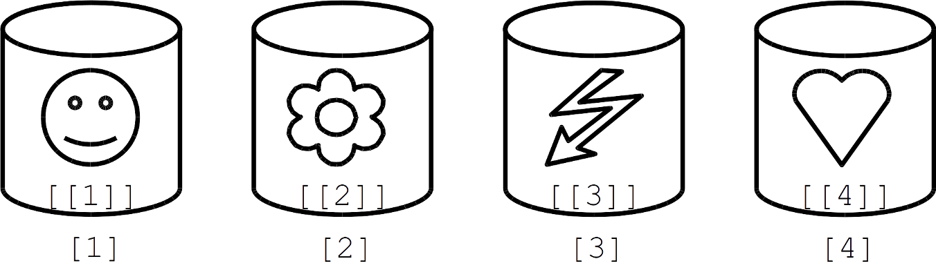
FIGURE 3.1: Schematic representation of a list of length four.
Figure 3.1 is a schematic representation of a list of
length four. The first bin [1] contains a smiling face [[1]], the
second bin [2] contains a flower [[2]], the third bin [3]
contains a lightning bolt [[3]], and the fourth bin [[4]] contains
a heart [[4]]. When indexing a list object, single brackets
[\(\cdot\)] indexes the bin, and double brackets [[\(\cdot\)]]
indexes the bin contents. If the bin has a name, then $name also
indexes the contents.
For example, using the UGDP clinical trial data,19 suppose we perform Fisher’s exact test for testing the null hypothesis of independence of rows and columns in a contingency table with fixed marginals.
#>           Treatment
#> Status     Tolbutamide Placebo
#>   Death             30      21
#> Survivor 174 184#>
#> Fisher's Exact Test for Count Data
#>
#> data: tab
#> p-value = 0.1813
#> alternative hypothesis: true odds ratio is not equal to 1
#> 95 percent confidence interval:
#> 0.8013768 2.8872863
#> sample estimates:
#> odds ratio
#> 1.509142The default display shows partial results. All the results are stored
in the object ftab. Let’s evaluate the structure of ftab and
extract some results:
#> List of 7
#>  $ p.value    : num 0.181
#>  $ conf.int   : num [1:2] 0.801 2.887
#>   ..- attr(*, "conf.level")= num 0.95
#>  $ estimate   : Named num 1.51
#>   ..- attr(*, "names")= chr "odds ratio"
#>  $ null.value : Named num 1
#>   ..- attr(*, "names")= chr "odds ratio"
#>  $ alternative: chr "two.sided"
#>  $ method     : chr "Fisher's Exact Test for Count Data"
#>  $ data.name  : chr "tab"
#> - attr(*, "class")= chr "htest"#> odds ratio
#> 1.509142#> [1] 0.8013768 2.8872863
#> attr(,"conf.level")
#> [1] 0.95#> [1] 0.1812576The str function returns the structure of the output object.
to extract additional results either for display or for further
analysis. In this case, ftab is a list with 7 bins, each with a
name.
3.1.2 Creating lists
To create a list directly, use the list function. Table
3.1 summarizes how to create lists.
| Function | Description | Try these examples |
|---|---|---|
list |
Creates list object | y <- matrix(4:1, 2,2) |
z <- c("Pedro", "Paulo") |
||
mm <- list(y, z); mm |
||
data.frame |
Vectors to tabular list | id <- 1:3 |
sex <- c("M","F", "M") |
||
df <- data.frame(id, sex); df |
||
as.data.frame |
Coercion | x <- matrix(1:6, 2, 3); x |
y <- as.data.frame(x); y |
||
read.table |
Read ASCII file | read.table('~/data/ugdp.txt') |
read.csv |
read.csv('~/data/ugdp.txt') |
|
vector |
Empty list length \(n\) | vector("list", 2) |
as.list |
Coercion into list | list(1:2) |
as.list(1:2) |
A great use for a list is to collecte the results of a function into an object. For example, here’s a function to calculate an odds ratio from a \(2 \times 2\) table:
orcalc <- function(x){
    or <- (x[1,1] * x[2,2]) /(x[1,2] * x[2,1])
    pval <- fisher.test(x)$p.value
    list(data = x, odds.ratio = or, p.value = pval)
}
The orcalc function has been loaded in R, and now we run the
function on the UGDP data.
#>           Treatment
#> Status     Tolbutamide Placebo
#>   Death             30      21
#> Survivor 174 184#> $data
#> Treatment
#> Status Tolbutamide Placebo
#> Death 30 21
#> Survivor 174 184
#>
#> $odds.ratio
#> [1] 1.510673
#>
#> $p.value
#> [1] 0.1812576For additional practice, study and implement the examples in Table 3.1.
3.1.3 Naming lists
| Function | Comment | Try these examples |
|---|---|---|
names |
After list creation | z <- list(rnorm(20), 'Luis'); z |
names(z) <- c('bin1', 'bin2') |
||
| At list creation | z <- list(bin1 = rnorm(20), bin2 = 'Luis') |
|
names(z) # returns names |
The components (or ‘bins’) of a list can be unnamed or named.
Components of a list can be named at the time the list is created or
later using the names function. For practice, try the
examples in Table 3.2.
3.1.4 Indexing lists
| Indexing | Try these examples |
|---|---|
| By position | z <- list(bin1 = rnorm(20), bin2 = 'Luiz') |
z[1] # indexes bin #1 |
|
z[[1]] # indexes contents of bin #1 |
|
| By name (if exists) | z$bin1 # indexes contents of bin #1 |
| By logical vector | num <- sapply(z, is.numeric); num |
z[num] |
If list components (bins) are unnamed, we can index the list by bin
position with single or double brackets. The single brackets
[\(\cdot\)] indexes one or more bins, and the double brackets
indexes contents of a single bin only.
#> [[1]]
#> [1] 1 2 3 4 5
#>
#> [[2]]
#> [1] "Juan" "Wilfredo"#> [1] "Juan" "Wilfredo"When list bins are named, we can index the bin contents by name.
Using the matched case-control study infert data set, we will
conduct a conditional logistic regression analysis to determine if
spontaneous and induced abortions are independently associated with
infertility. For this we’ll need to load the survival package which
contains the clogit function.
#> [1] "education"      "age"            "parity"
#> [4] "induced"        "case"           "spontaneous"
#> [7] "stratum"        "pooled.stratum"
mod1 <- clogit(case ~ spontaneous + induced + strata(stratum),
data = infert)
mod1 # default display of model#> Call:
#> clogit(case ~ spontaneous + induced + strata(stratum), data = infert)
#>
#> coef exp(coef) se(coef) z p
#> spontaneous 1.9859 7.2854 0.3524 5.635 1.75e-08
#> induced 1.4090 4.0919 0.3607 3.906 9.38e-05
#>
#> Likelihood ratio test=53.15 on 2 df, p=2.869e-12
#> n= 248, number of events= 83#> [1] TRUE#> [1] "coefficients" "var" "loglik"
#> [4] "score" "iter" "linear.predictors"
#> [7] "residuals" "means" "method"
#> [10] "n" "nevent" "terms"
#> [13] "assign" "wald.test" "concordance"
#> [16] "y" "formula" "xlevels"
#> [19] "call" "userCall"#> spontaneous induced
#> 1.985876 1.409012The stratum option is used to specify the field that identifies the
cases and their matched controls. The mod1 object has a default
display (shown). However, it is a list. We can use str to evaluate
the list structure. Instead names was used to display the list
component names. Sometimes it is more convenience to display the names
for the list rather than the complete structure.
The summary function applied to a regression model object creates a
list object with more detailed results. This too has a default
display, or we can index list components by name.
#> Call:
#> coxph(formula = Surv(rep(1, 248L), case) ~ spontaneous + induced +
#>     strata(stratum), data = infert, method = "exact")
#>
#>   n= 248, number of events= 83
#>
#>               coef exp(coef) se(coef)     z Pr(>|z|)
#> spontaneous 1.9859    7.2854   0.3524 5.635 1.75e-08 ***
#> induced     1.4090    4.0919   0.3607 3.906 9.38e-05 ***
#> ---
#> Signif. codes:  0 '***' 0.001 '**' 0.01 '*' 0.05 '.' 0.1 ' ' 1
#>
#>             exp(coef) exp(-coef) lower .95 upper .95
#> spontaneous     7.285     0.1373     3.651    14.536
#> induced         4.092     0.2444     2.018     8.298
#>
#> Concordance= 0.776  (se = 0.044 )
#> Likelihood ratio test= 53.15  on 2 df,   p=3e-12
#> Wald test            = 31.84  on 2 df,   p=1e-07
#> Score (logrank) test = 48.44 on 2 df, p=3e-11#> [1] "call" "fail" "na.action" "n"
#> [5] "loglik" "nevent" "coefficients" "conf.int"
#> [9] "logtest" "sctest" "rsq" "waldtest"
#> [13] "used.robust" "concordance"#> coef exp(coef) se(coef) z Pr(>|z|)
#> spontaneous 1.985876 7.285423 0.3524435 5.634592 1.754734e-08
#> induced 1.409012 4.091909 0.3607124 3.906191 9.376245e-053.1.5 Replacing lists components
| Replacing | Try these examples |
|---|---|
| By position | z <- list(bin1 = rnorm(20), bin2 = 'Luis') |
z[1] <- list(c(1, 2)) # replaces bin contents |
|
z[[1]] <- c(3, 4) # replaces bin contents |
|
| By name (if exists) | z$bin2 <- c("Tomas", "Luis", "Angela"); z |
# replace name of specific "bin" |
|
names(z)[2] <- "mykids"; z |
|
| By logical | num <- sapply(z, is.numeric); num |
z[num] <- list(rnorm(5)); z |
Replacing list components is accomplished by combining indexing with assignment. And of course, we can index by position, name, or logical. Remember, if it can be indexed, it can be replaced. Study and practice the examples in Table 3.4.
3.1.6 Operating on lists
Because lists can have complex structural components, there are not
many operations we will want to do on lists. When we want to apply a
function to each component (bin) of a list, we use the lapply
or sapply function. These functions are identical except
that sapply “simplifies” the final result, if possible.
| Function | Description with examples |
|---|---|
lapply |
Applies function to list and returns list |
x <- list(1:5, 6:10) |
|
lapply(x, mean) |
|
sapply |
Applies function to list and simplifies |
sapply(x, mean) |
|
do.call |
Calls and applies a function to the list |
do.call(rbind, x) |
|
mapply |
Applies a function to the 1st bin of each argument, the 2nd, the 3rd, and so on. |
x <- list(1:4, 1:4); y <- list(4, rep(4, 4)) |
|
mapply(rep, x, y, SIMPLIFY = FALSE) |
|
mapply(rep, x, y) |
The do.call function applies a function to the entire list
using each each component as an argument. For example, consider a
list where each bin contains a vector and we want to cbind
the vectors.
#>      mylist
#> vec1 Integer,5
#> vec2 Integer,5
#> vec3 Integer,5#> vec1 vec2 vec3
#> [1,] 1 6 11
#> [2,] 2 7 12
#> [3,] 3 8 13
#> [4,] 4 9 14
#> [5,] 5 10 15For additional practice, study and implements the examples in Table 3.5.
3.2 A data frame is a list in a 2-dimensional tabular form
A data frame is a list in 2-dimensional tabular form. Each list component (bin) is a data field of equal length. A data frame is a list that behaves like a matrix. Anything that can be done with lists can be done with data frames. Many operations that can be done with a matrix can be done with a data frame.
3.2.1 Understanding data frames and factors
Epidemiologists are familiar with tabular data sets where each row is
a record and each column is a field. A record can be data
collected on individuals or groups. We usually refer to the field
name as a variable (e.g., age, gender, ethnicity). Fields can contain
numeric or character data. In R, these types of data sets are handled
by data frames. Each column of a data frame is usually either a
factor or numeric vector, although it can have complex, character, or
logical vectors. Data frames have the functionality of matrices and
lists. For example, here is the first 10 rows of the infert data
set, a matched case-control study published in 1976 that evaluated
whether infertility was associated with prior spontaneous or induced
abortions.
#> 'data.frame':    248 obs. of  8 variables:
#>  $ education     : Factor w/ 3 levels "0-5yrs","6-11yrs",..: 1 1 1 1 2 2 2 2 2 2 ...
#>  $ age           : num  26 42 39 34 35 36 23 32 21 28 ...
#>  $ parity        : num  6 1 6 4 3 4 1 2 1 2 ...
#>  $ induced       : num  1 1 2 2 1 2 0 0 0 0 ...
#>  $ case          : num  1 1 1 1 1 1 1 1 1 1 ...
#>  $ spontaneous   : num  2 0 0 0 1 1 0 0 1 0 ...
#>  $ stratum       : int  1 2 3 4 5 6 7 8 9 10 ...
#> $ pooled.stratum: num 3 1 4 2 32 36 6 22 5 19 ...#> education age parity induced case spontaneous
#> 1 0-5yrs 26 6 1 1 2
#> 2 0-5yrs 42 1 1 1 0
#> 3 0-5yrs 39 6 2 1 0
#> 4 0-5yrs 34 4 2 1 0
#> 5 6-11yrs 35 3 1 1 1The fields are obviously vectors. Let’s explore a few of these vectors to see what we can learn about their structure in R.
#> [1] 26 42 39 34 35 36 23 32 21 28#> [1] "numeric"#> [1] "numeric"#> [1] 1 2 3 4 5 6 7 8 9 10#> [1] "numeric"#> [1] "integer"#> [1] 0-5yrs 0-5yrs 0-5yrs 0-5yrs 6-11yrs 6-11yrs
#> Levels: 0-5yrs 6-11yrs 12+ yrs#> [1] "numeric"#> [1] "factor"What have we learned so far? In the infert data frame,
age is a vector of mode “numeric” and class “numeric,”
stratum is a vector of mode `numeric'' and class "integer," andeducation` is a vector of mode “numeric”
and class “factor.” The numeric vectors are straightforward and
easy to understand. However, a factor, R’s representation of
categorical data, is a bit more complicated.
Contrary to intuition, a factor is an integer (numeric) vector, not a
character vector, although it may have been created from a character
vector (shown later). To see the “true” education factor use the
unclass function:
#> [1] 1 1 1 1 2 2 2 2 2 2Now let’s create a factor from a character vector and then unclass it:
#> [1] "Head" "Head" "Head" "Head" "Tail" "Head" "Tail"#> [1] Head Head Head Head Tail Head Tail
#> Levels: Head Tail#> [1] 1 1 1 1 2 1 2Notice that we can still recover the original character vector using
the as.character function:
#> [1] "Head" "Head" "Head" "Head" "Tail" "Head" "Tail"#> [1] "Head" "Head" "Head" "Head" "Tail" "Head" "Tail"Okay, let’s create an ordered factor; that is, levels of a
categorical variable that have natural ordering. For this we set
ordered = TRUE in the factor function:
samp <- sample(c('Low', 'Medium', 'High'), 100, replace = TRUE)
ofac1 <- factor(samp, ordered = TRUE)
ofac1[1:7]
#> [1] Medium High Medium Low Low Medium High
#> Levels: High < Low < Medium#> ofac1
#> High Low Medium
#> 36 29 35However, notice that the ordering was done in alphabetical
order which is not what we want. To correct this, use the
levels option in the factor function:
#> [1] Medium High   Medium Low    Low    Medium High
#> Levels: Low < Medium < High#> ofac2
#> Low Medium High
#> 29 35 36Great—this is exactly what we want! For review, Table
3.6 summarizes the variable types in epidemiology and how
they are represented in R. Factors (unordered and ordered) are used
to represent nominal and ordinal categorical data. The infert data
set contains nominal factors and the esoph data set contains ordinal
factors. Notice that in R the internal representation of categorical
variables are of mode numeric. We can see this using the unclass
function on the variable.
| Variable type | Examples | mode |
typeof |
class |
|---|---|---|---|---|
| Numeric | ||||
| Continuous | 1, 2, 3.45, 2/3 | numeric | double | numeric |
| Discrete | 1, 2, 3, 4, | numeric | integer | integer |
| Categorical | ||||
| Nominal | male vs. female | numeric | integer | factor |
| Ordinal | low < medium < high | numeric | integer | ordered factor |
3.2.2 Creating data frames
In the creation of data frames, character vectors (usually representing categorical data) are converted to factors (mode numeric, class factor), and numeric vectors are converted to numeric vectors of class numeric or class integer. Common ways of creating data frames are summarized in Table 3.7. Factors can be created directly from vectors.
wt <- c(59.5, 61.4, 45.2)
age <- c(11, 9, 6)
gender <- c('Male', 'Male', 'Female')
df <- data.frame(age, gender, wt); df
#> age gender wt
#> 1 11 Male 59.5
#> 2 9 Male 61.4
#> 3 6 Female 45.2#> 'data.frame': 3 obs. of 3 variables:
#> $ age : num 11 9 6
#> $ gender: Factor w/ 2 levels "Female","Male": 2 2 1
#> $ wt : num 59.5 61.4 45.2#>
#> Female Male
#> 1 2Notice that the character vector was automatically converted to a
factor. In this example, possible values of gender were derived
from the data vector. However, if possible values of gender
included “transgender” (although none were recorded), we can specify
this using using levels option.
#>
#>        Male      Female Transgender
#>           2           1           0
Factors allow us to keep track of possible values in categorical data even if specific values were not recorded in a given data set.
| Function | Description | Try these examples |
|---|---|---|
data.frame |
Create tabular list | id <- 1:2; sex <- c('M','F') |
x <- data.frame(id, sex) |
||
| Convert fully labeled array | data(Titanic) # load data |
|
data.frame(Titanic) |
||
as.data.frame |
Coercion | x <- matrix(1:6, 2, 3); x |
as.data.frame(x) |
||
read.table |
Reads ASCII text file | see help(read.table) |
expand.grid |
All combinations of vectors | see help(expand.grid) |
Sometimes we want to convert an array into a data frame for analysis or sharing. Consider the Titanic array data that come with R. We can convert an array to a data frame (first 6 rows shown):
#> , , Survived = No
#>
#>       Sex
#> Class  Male Female
#>   1st     0      0
#>   2nd     0      0
#>   3rd    35     17
#>   Crew    0      0
#>
#> , , Survived = Yes
#>
#>       Sex
#> Class  Male Female
#>   1st     5      1
#>   2nd    11     13
#>   3rd    13     14
#> Crew 0 0#> Class Sex Age Survived Freq
#> 1 1st Male Child No 0
#> 2 2nd Male Child No 0
#> 3 3rd Male Child No 35
#> 4 Crew Male Child No 0
#> 5 1st Female Child No 0
#> 6 2nd Female Child No 03.2.3 Naming data frames
| Function | Try these examples |
|---|---|
| names | x <- data.frame(var1 = 1:3, var2 = c('M', 'F', 'F')) |
names(x) <- c('Subjno', 'Sex') |
|
| row.names | row.names(x) <- c('Sub 1', 'Sub 2', 'Sub 3'); x |
Everything that applies to naming list components (Table 3.2) also applies to naming data frame components (Table 3.8). In general, we may be interested in renaming variables (fields) or row names of a data frame, or renaming the levels (possible values) for a given factor (categorical variable). For example, consider the Oswego data set.
odat <- read.table('~/data/oswego.txt', sep = '', header = TRUE,
                   na.strings = '.')
odat[1:5,1:8]              #Display partial data frame
#> id age sex meal.time ill onset.date onset.time baked.ham
#> 1 2 52 F 8:00 PM Y 4/19 12:30 AM Y
#> 2 3 65 M 6:30 PM Y 4/19 12:30 AM Y
#> 3 4 59 F 6:30 PM Y 4/19 12:30 AM Y
#> 4 6 63 F 7:30 PM Y 4/18 10:30 PM Y
#> 5 7 70 M 7:30 PM Y 4/18 10:30 PM Ynames(odat)[3] <- 'Gender' #Rename 'sex' to 'Gender'
table(odat$Gender) #Display 'Gender' distribution#>
#> F M
#> 44 31#> [1] "F" "M" # Replace 'Gender' level labels
levels(odat$Gender) <- c('Female', 'Male')
levels(odat$Gender) #Display new 'Gender' levels#> [1] "Female" "Male"#>
#> Female Male
#> 44 31#> id age Gender meal.time ill onset.date
#> 1 2 52 Female 8:00 PM Y 4/19
#> 2 3 65 Male 6:30 PM Y 4/19
#> 3 4 59 Female 6:30 PM Y 4/19
#> 4 6 63 Female 7:30 PM Y 4/18On occasion, we might be interested in renaming the row names. Currently, the Oswego data set has default integer values from 1 to 75 as the row names.
#> [1] "1" "2" "3" "4" "5" "6" "7" "8" "9" "10"We can change the row names by assigning a new character vector.
#>     id age Gender meal.time ill onset.date
#> 199  2  52 Female   8:00 PM   Y       4/19
#> 179  3  65   Male   6:30 PM   Y       4/19
#> 130  4  59 Female   6:30 PM   Y       4/19
#> 191  6  63 Female   7:30 PM   Y       4/18
3.2.4 Indexing data frames
| Indexing | Try these examples |
|---|---|
| By position | data(infert) |
infert[1:5, 1:3] |
|
| By name | infert[1:5, c("education", "age", "parity")] |
| By logical | agelt30 <- infert$age < 30 # create logical vector |
infert[agelt30, c("education", "induced", "parity")] |
|
# can also use 'subset' function |
|
subset(infert, agelt30, c("education", "induced", "parity")) |
Indexing a data frame is similar to indexing a matrix or a list: we can index by position, by name, or by logical vector. Consider, for example, the 2004 California West ile virus human disease surveillance data. Suppose we are interested in summarizing the Los Angeles cases with neuroinvasive disease (“WNND”).
#> 'data.frame':    779 obs. of  8 variables:
#>  $ id         : int  1 2 3 4 5 6 7 8 9 10 ...
#>  $ county     : Factor w/ 23 levels "Butte","Fresno",..: 14 14 14 14 14 14 14 14 8 12 ...
#>  $ age        : int  40 64 19 12 12 17 61 74 71 26 ...
#>  $ sex        : Factor w/ 2 levels "F","M": 1 1 2 2 2 2 2 1 2 2 ...
#>  $ syndrome   : Factor w/ 3 levels "Unknown","WNF",..: 2 2 2 2 2 2 3 3 2 3 ...
#>  $ date.onset : Factor w/ 130 levels "2004-05-14","2004-05-16",..: 3 4 4 2 1 5 7 10 7 9 ...
#>  $ date.tested: Factor w/ 104 levels "2004-06-02","2004-06-16",..: 1 2 2 2 2 3 4 5 6 6 ...
#> $ death : Factor w/ 2 levels "No","Yes": 1 1 1 1 1 1 1 1 1 1 ...#> [1] "Butte" "Fresno" "Glenn"
#> [4] "Imperial" "Kern" "Lake"
#> [7] "Lassen" "Los Angeles" "Merced"
#> [10] "Orange" "Placer" "Riverside"
#> [13] "Sacramento" "San Bernardino" "San Diego"
#> [16] "San Joaquin" "Santa Clara" "Shasta"
#> [19] "Sn Luis Obispo" "Tehama" "Tulare"
#> [22] "Ventura" "Yolo"#> [1] "Unknown" "WNF" "WNND"myrows <- wdat$county=="Los Angeles" & wdat$syndrome=="WNND"
mycols <- c("id", "county", "age", "sex", "syndrome", "death")
wnv.la <- wdat[myrows, mycols]
wnv.la[1:6, ]#> id county age sex syndrome death
#> 25 25 Los Angeles 70 M WNND No
#> 26 26 Los Angeles 59 M WNND No
#> 27 27 Los Angeles 59 M WNND No
#> 47 47 Los Angeles 57 M WNND No
#> 48 48 Los Angeles 60 M WNND No
#> 49 49 Los Angeles 34 M WNND NoIn this example, the data frame rows were indexed by logical vector, and the columns were indexed by names. We emphasize this method because it only requires application of previously learned principles that always work with R objects.
An alternative method is to use the subset function. The first
argument specifies the data frame, the second argument is a Boolean
operation that evaluates to a logical vector, and the third argument
specifies what variables (or range of variables) to include or
exclude.
wnv.sf2 <- subset(wdat, county=="Los Angeles" & syndrome=="WNND",
                  select=c(id, county, age, sex, syndrome, death))
wnv.sf2[1:6,]
#> id county age sex syndrome death
#> 25 25 Los Angeles 70 M WNND No
#> 26 26 Los Angeles 59 M WNND No
#> 27 27 Los Angeles 59 M WNND No
#> 47 47 Los Angeles 57 M WNND No
#> 48 48 Los Angeles 60 M WNND No
#> 49 49 Los Angeles 34 M WNND NoThis example is equivalent but specifies range of variables using the
: function:
wnv.sf3 <- subset(wdat, county=="Los Angeles" & syndrome=="WNND",
                  select = c(id:syndrome, death))
wnv.sf3[1:6,]
#> id county age sex syndrome death
#> 25 25 Los Angeles 70 M WNND No
#> 26 26 Los Angeles 59 M WNND No
#> 27 27 Los Angeles 59 M WNND No
#> 47 47 Los Angeles 57 M WNND No
#> 48 48 Los Angeles 60 M WNND No
#> 49 49 Los Angeles 34 M WNND NoThis example is equivalent but specifies variables to exclude using
the - function:
wnv.sf4 <- subset(wdat, county=="Los Angeles" & syndrome=="WNND",
                  select = -c(date.onset, date.tested))
wnv.sf4[1:6, ]
#> id county age sex syndrome death
#> 25 25 Los Angeles 70 M WNND No
#> 26 26 Los Angeles 59 M WNND No
#> 27 27 Los Angeles 59 M WNND No
#> 47 47 Los Angeles 57 M WNND No
#> 48 48 Los Angeles 60 M WNND No
#> 49 49 Los Angeles 34 M WNND NoThe subset function offers some conveniences such as the ability to
specify a range of fields to include using the : function, and to
specify a group of fields to exclude using the - function.
3.2.5 Replacing data frame components
| Replacing | Try these examples |
|---|---|
| By position | data(infert) |
infert[1:4, 1:2] |
|
infert[1:4, 2] <- c(NA, 45, NA, 23) |
|
infert[1:4, 1:2] |
|
| By name | names(infert) |
infert[1:4, c("education", "age")] |
|
infert[1:4, c("age")] <- c(NA, 45, NA, 23) |
|
infert[1:4, c("education", "age")] |
|
| By logical | table(infert$parity) |
# change values of 5 or 6 to missing (NA) |
|
infert$parity[infert$parity==5 | infert$parity==6]<-NA |
|
table(infert$parity) |
|
table(infert$parity, exclude = NULL) |
With data frames, as with all R data objects, anything that can be indexed can be replaced. We already saw some examples of replacing names. For practice, study and implement the examples in Table 3.10.
3.2.6 Operating on data frames
| Function | Description with examples |
|---|---|
tapply |
Applies function to strata of a vector |
data(infert) |
|
args(tapply) # display argument |
|
tapply(infert$age, infert$educ, mean, na.rm=TRUE) |
|
lapply |
Applies function to list and returns list |
lapply(infert[, 1:3], table) |
|
sapply |
Applies function to list and simplifies |
sapply(infert[,c("age","parity")],mean,na.rm=TRUE) |
|
aggregate |
Split data into subsets, and computes statistic for each |
aggregate(infert[, c("age", "parity")], by = list(Education = infert$education, Induced = infert$induced), mean) |
|
mapply |
Applies function to \(x\) bin of each argument, for \(x=1,2,\cdots\) |
df <- data.frame(var1 = 1:4, var2 = 4:1) |
|
mapply("*", df$var1, df$var2) |
|
mapply(c, df$var1, df$var2) |
|
mapply(c, df$var1, df$var2, SIMPLIFY = FALSE) |
A data frame is of mode list, and functions that operate on components of a list will work with data frames. For example, consider the year California population estimates for the year 2000.
#> 'data.frame':    11918 obs. of  11 variables:
#>  $ County   : int  1 1 1 1 1 1 1 1 1 1 ...
#>  $ Year     : int  2000 2000 2000 2000 2000 2000 2000 2000 2000 2000 ...
#>  $ Sex      : Factor w/ 2 levels "F","M": 1 1 1 1 1 1 1 1 1 1 ...
#>  $ Age      : int  0 1 2 3 4 5 6 7 8 9 ...
#>  $ White    : int  2751 2673 2654 2646 2780 2826 2871 2942 3087 3070 ...
#>  $ Hispanic : int  2910 2837 2770 2798 2762 2738 2872 2837 2756 2603 ...
#>  $ Asian    : int  1921 1820 1930 1998 2029 1998 1984 1993 1957 2031 ...
#>  $ Pac.Isl  : int  63 70 64 64 85 93 78 94 85 83 ...
#>  $ Black    : int  1346 1343 1442 1455 1558 1632 1657 1732 1817 1819 ...
#>  $ Amer.Ind : int  32 37 37 39 38 45 53 51 43 44 ...
#> $ Multirace: int 711 574 579 588 575 576 548 514 545 537 ...#> County Year Sex Age White Hispanic Asian Pac.Isl
#> 1 1 2000 F 0 2751 2910 1921 63
#> 2 1 2000 F 1 2673 2837 1820 70
#> 3 1 2000 F 2 2654 2770 1930 64
#> 4 1 2000 F 3 2646 2798 1998 64
#> 5 1 2000 F 4 2780 2762 2029 85Now, suppose we want to assess the range of the numeric fields. If we
treat the data frame as a list, both lapply or sapply
works. Excluding the “Sex” variable, the following code will return the
range (i.e., minimum and maximum values) of the capop data frame.
However, if we treat the data frame as a matrix, apply also works:
#>      County Year Age  White Hispanic Asian Pac.Isl Black
#> [1,]      1 2000   0      0        0     0       0     0
#> [2,]     59 2000 100 148246   127415 35240    1066 21865
#>      Amer.Ind Multirace
#> [1,]        0         0
#> [2,]     1833     11299
Some R functions, such as summary, will summarize every
variable in a data frame without having to use lapply or
sapply.
#>      County        Year      Sex           Age
#>  Min.   : 1   Min.   :2000   F:5959   Min.   :  0
#>  1st Qu.:15   1st Qu.:2000   M:5959   1st Qu.: 25
#>  Median :30   Median :2000            Median : 50
#>  Mean   :30   Mean   :2000            Mean   : 50
#>  3rd Qu.:45   3rd Qu.:2000            3rd Qu.: 75
#>  Max.   :59   Max.   :2000            Max.   :100
#>      White           Hispanic            Asian
#>  Min.   :     0   Min.   :     0.0   Min.   :    0.0
#>  1st Qu.:   100   1st Qu.:    10.0   1st Qu.:    2.0
#>  Median :   385   Median :    76.0   Median :   16.0
#>  Mean   :  2693   Mean   :  1859.9   Mean   :  628.7
#>  3rd Qu.:  1442   3rd Qu.:   589.8   3rd Qu.:  139.0
#>  Max.   :148246   Max.   :127415.0   Max.   :35240.0
3.2.6.1 The aggregate function
The aggregate function is almost identical to the tapply function.
Recall that tapply allows us to apply a function to a single
vector that is stratified by one or more fields; for example,
calculating mean age (1 field) stratified by sex and ethnicity (2
fields). In contrast, aggregate allows us to apply a function to a
group of fields that are stratified by one or more fields; for
example, calculating the mean weight and height (2 fields) stratified
by sex and ethnicity (2 fields):
sex <- c("M", "M", "M", "M", "F", "F", "F", "F")
eth <- c("W", "W", "B", "B", "W", "W", "B", "B")
wgt <- c(140, 150, 150, 160, 120, 130, 130, 140)
hgt <- c( 60,  70,  70,  80,  40,  50,  50,  60)
df <- data.frame(sex, eth, wgt, hgt)
aggregate(df[, 3:4], by = list(Gender = df$sex,
                Ethnicity = df$eth), FUN = mean)
#> Gender Ethnicity wgt hgt
#> 1 F B 135 55
#> 2 M B 155 75
#> 3 F W 125 45
#> 4 M W 145 65For another example, in the capop data frame, we notice that the
variable age goes from 0 to 100 by 1-year intervals. It will be useful
to aggregate ethnic-specific population estimates into larger age
categories. More specifically, we want to calculate the sum of
ethnic-specific population estimates (6 fields) stratified by age
category, sex, and year (3 fields). We will create a new 7-level age
category field commonly used by the National Center for Health
Statistics. Naturally, we use the aggregate function:
to.keep <- c("White", "Hispanic", "Asian", "Pac.Isl",
             "Black", "Amer.Ind", "Multirace")
age.nchs7 <- c(0, 1, 5, 15, 25, 45, 65, 101)
capop$agecat7 <- cut(capop$Age, breaks = age.nchs7, right = FALSE)
capop7 <- aggregate(capop[,to.keep], by = list(Age = capop$agecat7,
                    Sex = capop$Sex, Year = capop$Year), FUN = sum)
levels(capop7$Age)[7] <- "65+"
capop7[1:14, 1:6]
#> Age Sex Year White Hispanic Asian
#> 1 [0,1) F 2000 151238 231822 41758
#> 2 [1,5) F 2000 627554 929222 172296
#> 3 [5,15) F 2000 1849860 2249146 482094
#> 4 [15,25) F 2000 1737534 1893896 545692
#> 5 [25,45) F 2000 4720500 3484732 1335912
#> 6 [45,65) F 2000 4204180 1470124 890078
#> 7 65+ F 2000 2943684 559730 417132
#> 8 [0,1) M 2000 159360 243170 43930
#> 9 [1,5) M 2000 662386 968136 182746
#> 10 [5,15) M 2000 1958466 2350768 515148
#> 11 [15,25) M 2000 1850710 2161736 558628
#> 12 [25,45) M 2000 4930388 3843792 1229216
#> 13 [45,65) M 2000 4149666 1375098 768022
#> 14 65+ M 2000 2150452 404598 3099323.3 Managing data objects and workspace
When we work in R we have a workspace. Think of the workspace as our
office desk top that have the “objects” (data and tools) we use to
conduct our work. To view all the objects in our workspace use ls()
or objects() To view objects that match a pattern use the pattern
option. To remove all data objects use rm(list = ls()) with extreme
caution. See Table 3.12 for summary.
#> [1] "obj1" "obj2" "obj3" "obj4" "obj5"#> [1] "obj1" "obj3" "obj5"| Function | Description and examples |
|---|---|
ls, objects |
List objects |
rm, remove |
Remove object(s) |
save.image |
Saves workspace |
save |
Saves objects to external file. |
load |
Loads objects previously saved |
Object names in the workspace may not be sufficiently descriptive to
know what these objects contain. To assess R objects in our workspace
we use the functions summarized in Table 3.13.
In general, we never go wrong using the str, mode, and class
functions.
Objects created in the workspace are available during the R session.
Upon closing the R session, R asks whether to save the workspace. To
save the objects without exiting an R session, use save.image().
The save.image function is actually a special case of the save
function:
The save function saves an R object as an external file. This file
can be loaded using the load function.
x <- runif(20); y <- list(a = 1, b = TRUE, c = "oops")
save(x, y, file = "xy.RData") # external file
ls() # display objects in current workking directory
#> [1] "x" "y"#> character(0)#> [1] "x" "y"unlink("xy.RData") # unlinks and removes external file
ls() # 'x' and 'y' remain in current working directory#> [1] "x" "y"| Query object | Coerce to type | Query object | Coerce to type | ||||
|---|---|---|---|---|---|---|---|
is.vector |
as.vector |
is.integer |
as.integer |
||||
is.matrix |
as.matrix |
is.character |
as.character |
||||
is.array |
as.array |
is.logical |
as.logical |
||||
is.list |
as.list |
is.function |
as.function |
||||
is.data.frame |
as.data.frame |
is.null |
as.null |
||||
is.factor |
as.factor |
is.na |
n/a | ||||
is.ordered |
as.ordered |
is.nan |
n/a | ||||
is.table |
as.table |
is.finite |
n/a | ||||
is.numeric |
as.numeric |
is.infinite |
n/a |
Table 3.13 provides more functions for conducting specific object queries and for coercing one object type into another. For example, a vector is not a matrix.
#> [1] FALSEHowever, a vector can be coerced into a matrix.
#>      [,1]
#> [1,]    1
#> [2,]    2
#> [3,] 3#> [1] TRUEA common use would be to coerce a factor into a character vector.
#> [1] M M M M F F F
#> Levels: F M#> [1] 2 2 2 2 1 1 1
#> attr(,"levels")
#> [1] "F" "M"#> [1] "M" "M" "M" "M" "F" "F" "F"In R, missing values are represented by the value NA (“not
available”). The is.na function evaluates an object and
returns a logical vector indicating which positions contain
NA. The !is.na version returns positions that do
not contain NA.
#> [1] FALSE FALSE TRUE FALSE FALSE#> [1] TRUE TRUE FALSE TRUE TRUEWe can use is.na to replace missing values.
#> [1] 12 34 999 56 89In R, NaN represents “not a number” and Inf
represent an infinite value. Therefore, we can use is.nan and
is.infinite to assess which positions contain NaN
and Inf, respectively.
#> [1] 0 Inf NaN -Inf#> [1] FALSE FALSE TRUE FALSE#> [1] FALSE TRUE FALSE TRUEOur workspace is like a desktop that contains the “objects” (data
and tools) we use to conduct our work. Use the getwd function
to list the file path to the workspace file .RData.
#> [1] "/Users/tja/Dropbox/tja/Rproj/home"Use the setwd function to set up a new workspace location. A
(.RData) file will automatically be created there.
This is one method to manage multiple workspaces for one’s projects.
3.4 Exercises
Some of the exercises uses data that is available from
https://github.com/taragonmd/data. For example, suppose we are
interested in the mi.txt data. Locate the data set and select “Raw”
tab to view the raw data. Copy the URL for reading the data into our R
environment. Here is the URL for mi.txt:
https://raw.githubusercontent.com/taragonmd/data/master/mi.txt.
Exercise 3.1 (Data-driven decision making) Consider an observational study where 700 patients were given access to a new drug for an ailment. A total of 350 patients chose to take the drug and 350 patients did not. The patients were assessed for clinical recovery. Table 3.14
| Men | Women | ||||||
|---|---|---|---|---|---|---|---|
| Drug | No drug | Total | Drug | No drug | Total | ||
| Recovered | 81 | 234 | 315 | 192 | 55 | 247 | |
| No recovery | 6 | 36 | 42 | 71 | 25 | 96 | |
| Total at risk | 87 | 270 | 357 | 263 | 80 | 343 |
jp2 <-
read.csv('https://raw.githubusercontent.com/taragonmd/data/master/drugrx-pearl2.csv')
str(jp2)
#> 'data.frame': 700 obs. of 4 variables:
#> $ X : int 1 2 3 4 5 6 7 8 9 10 ...
#> $ Recovered: Factor w/ 2 levels "No","Yes": 2 2 2 2 2 2 2 2 2 2 ...
#> $ Drug : Factor w/ 2 levels "No","Yes": 2 2 2 2 2 2 2 2 2 2 ...
#> $ Gender : Factor w/ 2 levels "Men","Women": 1 1 1 1 1 1 1 1 1 1 ...#> , , Gender = Men
#>
#> Drug
#> Recovered No Yes
#> No 36 6
#> Yes 234 81
#>
#> , , Gender = Women
#>
#> Drug
#> Recovered No Yes
#> No 25 71
#> Yes 55 192For the variables Recovered (R), Drug (D), and Gender (G), use R to calculate the following probabilities (proportions).
- \(P(R = yes \mid D = no)\)
- \(P(R = yes \mid D = yes)\)
- \(P(R = yes \mid D = no, G = men)\)
- \(P(R = yes \mid D = yes, G = men)\)
- \(P(R = yes \mid D = no, G = women)\)
- \(P(R = yes \mid D = yes, G = women)\)
Discuss your findings and make drug treatment recommendations, and your rationale.
read.csv function to read in syphilis counts from 1989. Do
not attach the data frame (yet).
- Evaluate the structure of data frame.
- Create a 3-dimensional array using both the
tableandxtabsfunction.
apply function to get marginal totals for the syphilis
3-dimensional array (Sex by Race by Age).
sweep and apply functions to get marginal and joint
distributions for a 3-D array.
Use the rep function and the concept of indexing rows of a data
frame to recreate the individual-level data frame with over 40,000
observations. Instead of indexing to subset rows of a data frame, we
are indexing to replicate rows of a group-level data frame using the
frequency counts.
#### 1 Read county names
url1 <-
"https://raw.githubusercontent.com/taragonmd/data/master/calcounty.txt"
cty <- scan(url1, what="")

#### 2 Read county population estimates
url2 <-
"https://raw.githubusercontent.com/taragonmd/data/master/CalCounty2000.csv"
calpop <- read.csv(url2)

#### 2 Replace county number with county name
calpop$CtyName <- calpop$County ## create duplicate
for(i in 1:length(cty)){
    calpop$CtyName[calpop$County==i] <- cty[i]
}

#### 3 Discretize age into categories
calpop$Agecat <- cut(calpop$Age, c(0,20,45,65,100),
                     include.lowest = TRUE, right = FALSE)

#### 4 Create combined API category
calpop$AsianPI <- calpop$Asian + calpop$Pac.Isl

#### 5 Shorten selected ethnic labels
names(calpop)[c(6, 9, 10)] = c("Latino", "AfrAmer", "AmerInd")

#### 6 Index Bay Area Counties
baindex <- calpop$CtyName=="Alameda" | calpop$CtyName=="San Francisco"
bapop <- calpop[baindex,]
bapop

#### 7 Labels for later use
agelabs <- names(table(bapop$Agecat))
sexlabs <- c("Female", "Male")
racen <- c("White", "AfrAmer", "AsianPI", "Latino", "Multirace",
           "AmerInd")
ctylabs <- names(table(bapop$CtyName))

#### 8 Aggregate
bapop2 <- aggregate(bapop[,racen], list(Agecat = bapop$Agecat,
                   Sex = bapop$Sex, County = bapop$CtyName), sum)
bapop2

#### 9 Temp matrix of counts
tmp <- as.matrix(cbind(bapop2[1:4,racen], bapop2[5:8,racen],
             bapop2[9:12,racen], bapop2[13:16,racen]))

#### 10 Convert into final array
bapop3 <- array(tmp, c(4, 6, 2, 2))
dimnames(bapop3) <- list(agelabs, racen, sexlabs, ctylabs)
bapop3