Chapter 6 Tidy Data with Tidyr
Topics covered:
- gather
- spread
- separate
- complete
- fill
6.1 visualizing data
#rate per 10,000
table1%>%
  mutate(rate=cases/population*10000)
## # A tibble: 6 x 5
## country year cases population rate
## <chr> <int> <int> <int> <dbl>
## 1 Afghanistan 1999 745 19987071 0.373
## 2 Afghanistan 2000 2666 20595360 1.29
## 3 Brazil 1999 37737 172006362 2.19
## 4 Brazil 2000 80488 174504898 4.61
## 5 China 1999 212258 1272915272 1.67
## 6 China 2000 213766 1280428583 1.67#cases per year
table1%>%
count(year, wt=cases)## # A tibble: 2 x 2
## year n
## * <int> <int>
## 1 1999 250740
## 2 2000 296920library(ggplot2)
ggplot(table1, aes(year, cases))+
geom_line(aes(group=country), color='grey50')+
geom_point(aes(color=country))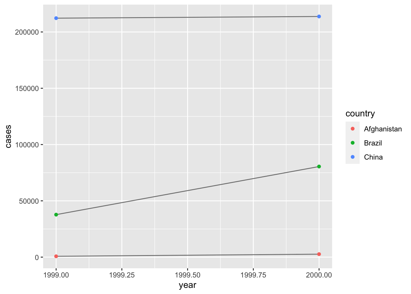
6.2 gather
#gathering
(tidy_4a <- table4a%>%
  gather('1999', '2000', key = 'year', value = 'cases'))
## # A tibble: 6 x 3
## country year cases
## <chr> <chr> <int>
## 1 Afghanistan 1999 745
## 2 Brazil 1999 37737
## 3 China 1999 212258
## 4 Afghanistan 2000 2666
## 5 Brazil 2000 80488
## 6 China 2000 213766(tidy_4b <- table4b%>%
gather('1999', '2000', key = 'year', value = 'population'))## # A tibble: 6 x 3
## country year population
## <chr> <chr> <int>
## 1 Afghanistan 1999 19987071
## 2 Brazil 1999 172006362
## 3 China 1999 1272915272
## 4 Afghanistan 2000 20595360
## 5 Brazil 2000 174504898
## 6 China 2000 1280428583left_join(tidy_4a, tidy_4b)## Joining, by = c("country", "year")## # A tibble: 6 x 4
## country year cases population
## <chr> <chr> <int> <int>
## 1 Afghanistan 1999 745 19987071
## 2 Brazil 1999 37737 172006362
## 3 China 1999 212258 1272915272
## 4 Afghanistan 2000 2666 20595360
## 5 Brazil 2000 80488 174504898
## 6 China 2000 213766 12804285836.3 spread
#spreading
#key is the variable we aim to spread
table2
## # A tibble: 12 x 4
## country year type count
## <chr> <int> <chr> <int>
## 1 Afghanistan 1999 cases 745
## 2 Afghanistan 1999 population 19987071
## 3 Afghanistan 2000 cases 2666
## 4 Afghanistan 2000 population 20595360
## 5 Brazil 1999 cases 37737
## 6 Brazil 1999 population 172006362
## 7 Brazil 2000 cases 80488
## 8 Brazil 2000 population 174504898
## 9 China 1999 cases 212258
## 10 China 1999 population 1272915272
## 11 China 2000 cases 213766
## 12 China 2000 population 1280428583spread(table2, key = type, value = count)## # A tibble: 6 x 4
## country year cases population
## <chr> <int> <int> <int>
## 1 Afghanistan 1999 745 19987071
## 2 Afghanistan 2000 2666 20595360
## 3 Brazil 1999 37737 172006362
## 4 Brazil 2000 80488 174504898
## 5 China 1999 212258 1272915272
## 6 China 2000 213766 12804285836.4 separate
#separate
table3
## # A tibble: 6 x 3
## country year rate
## * <chr> <int> <chr>
## 1 Afghanistan 1999 745/19987071
## 2 Afghanistan 2000 2666/20595360
## 3 Brazil 1999 37737/172006362
## 4 Brazil 2000 80488/174504898
## 5 China 1999 212258/1272915272
## 6 China 2000 213766/1280428583table3 %>%
separate(rate, into = c("cases", 'population'))## # A tibble: 6 x 4
## country year cases population
## <chr> <int> <chr> <chr>
## 1 Afghanistan 1999 745 19987071
## 2 Afghanistan 2000 2666 20595360
## 3 Brazil 1999 37737 172006362
## 4 Brazil 2000 80488 174504898
## 5 China 1999 212258 1272915272
## 6 China 2000 213766 1280428583#by default, separate at non-alphanumeric character
table3%>%
separate(rate, into = c('cases', 'population'), sep = '/')## # A tibble: 6 x 4
## country year cases population
## <chr> <int> <chr> <chr>
## 1 Afghanistan 1999 745 19987071
## 2 Afghanistan 2000 2666 20595360
## 3 Brazil 1999 37737 172006362
## 4 Brazil 2000 80488 174504898
## 5 China 1999 212258 1272915272
## 6 China 2000 213766 1280428583table3%>%
separate(rate, into = c('cases', 'population'), sep = '/',
convert = T)## # A tibble: 6 x 4
## country year cases population
## <chr> <int> <int> <int>
## 1 Afghanistan 1999 745 19987071
## 2 Afghanistan 2000 2666 20595360
## 3 Brazil 1999 37737 172006362
## 4 Brazil 2000 80488 174504898
## 5 China 1999 212258 1272915272
## 6 China 2000 213766 1280428583table3%>%
separate(year, into = c('century', 'year'), sep = 2)## # A tibble: 6 x 4
## country century year rate
## <chr> <chr> <chr> <chr>
## 1 Afghanistan 19 99 745/19987071
## 2 Afghanistan 20 00 2666/20595360
## 3 Brazil 19 99 37737/172006362
## 4 Brazil 20 00 80488/174504898
## 5 China 19 99 212258/1272915272
## 6 China 20 00 213766/12804285836.5 unite
#unite
table5%>%
  unite(new, century, year)
## # A tibble: 6 x 3
## country new rate
## <chr> <chr> <chr>
## 1 Afghanistan 19_99 745/19987071
## 2 Afghanistan 20_00 2666/20595360
## 3 Brazil 19_99 37737/172006362
## 4 Brazil 20_00 80488/174504898
## 5 China 19_99 212258/1272915272
## 6 China 20_00 213766/1280428583#by default sep=underscore
table5%>%
unite(new, century, year, sep = '')## # A tibble: 6 x 3
## country new rate
## <chr> <chr> <chr>
## 1 Afghanistan 1999 745/19987071
## 2 Afghanistan 2000 2666/20595360
## 3 Brazil 1999 37737/172006362
## 4 Brazil 2000 80488/174504898
## 5 China 1999 212258/1272915272
## 6 China 2000 213766/1280428583#missing value
(stocks <- tibble(
year=rep(c(2015,2016), each=4)[-8],
qtr=rep(1:4, times=2)[-5],
return=c(1.88, 0.59, 0.35, NA, 0.92, 0.17, 2.66)
))## # A tibble: 7 x 3
## year qtr return
## <dbl> <int> <dbl>
## 1 2015 1 1.88
## 2 2015 2 0.59
## 3 2015 3 0.35
## 4 2015 4 NA
## 5 2016 2 0.92
## 6 2016 3 0.17
## 7 2016 4 2.66stocks%>%
spread(key=year, value=return)## # A tibble: 4 x 3
## qtr `2015` `2016`
## <int> <dbl> <dbl>
## 1 1 1.88 NA
## 2 2 0.59 0.92
## 3 3 0.35 0.17
## 4 4 NA 2.66stocks%>%
spread(year, return)%>%
gather('2015', '2016', key = 'year', value = 'return', na.rm = T)## # A tibble: 6 x 3
## qtr year return
## <int> <chr> <dbl>
## 1 1 2015 1.88
## 2 2 2015 0.59
## 3 3 2015 0.35
## 4 2 2016 0.92
## 5 3 2016 0.17
## 6 4 2016 2.66#stocks%>%
# spread(year, return)%>%
# gather(year, return, '2015','2016', na.rm = T)
#complete cases
#identify unique combinations
stocks%>%
complete(year, qtr)## # A tibble: 8 x 3
## year qtr return
## <dbl> <int> <dbl>
## 1 2015 1 1.88
## 2 2015 2 0.59
## 3 2015 3 0.35
## 4 2015 4 NA
## 5 2016 1 NA
## 6 2016 2 0.92
## 7 2016 3 0.17
## 8 2016 4 2.66#fill
(treatment <- tribble(
~person, ~treatment, ~response,
"Derrick Whitemore", 1, 7,
NA, 2, 10,
NA, 3, 9,
"Katherine Burke", 1, 4
))## # A tibble: 4 x 3
## person treatment response
## <chr> <dbl> <dbl>
## 1 Derrick Whitemore 1 7
## 2 <NA> 2 10
## 3 <NA> 3 9
## 4 Katherine Burke 1 4#last observation carried forward
treatment %>%
fill(person)## # A tibble: 4 x 3
## person treatment response
## <chr> <dbl> <dbl>
## 1 Derrick Whitemore 1 7
## 2 Derrick Whitemore 2 10
## 3 Derrick Whitemore 3 9
## 4 Katherine Burke 1 4#an example
who## # A tibble: 7,240 x 60
## country iso2 iso3 year new_sp_m014 new_sp_m1524 new_sp_m2534 new_sp_m3544 new_sp_m4554 new_sp_m5564 new_sp_m65
## <chr> <chr> <chr> <int> <int> <int> <int> <int> <int> <int> <int>
## 1 Afghan… AF AFG 1980 NA NA NA NA NA NA NA
## 2 Afghan… AF AFG 1981 NA NA NA NA NA NA NA
## 3 Afghan… AF AFG 1982 NA NA NA NA NA NA NA
## 4 Afghan… AF AFG 1983 NA NA NA NA NA NA NA
## 5 Afghan… AF AFG 1984 NA NA NA NA NA NA NA
## 6 Afghan… AF AFG 1985 NA NA NA NA NA NA NA
## 7 Afghan… AF AFG 1986 NA NA NA NA NA NA NA
## 8 Afghan… AF AFG 1987 NA NA NA NA NA NA NA
## 9 Afghan… AF AFG 1988 NA NA NA NA NA NA NA
## 10 Afghan… AF AFG 1989 NA NA NA NA NA NA NA
## # … with 7,230 more rows, and 49 more variables: new_sp_f014 <int>, new_sp_f1524 <int>, new_sp_f2534 <int>,
## # new_sp_f3544 <int>, new_sp_f4554 <int>, new_sp_f5564 <int>, new_sp_f65 <int>, new_sn_m014 <int>, new_sn_m1524 <int>,
## # new_sn_m2534 <int>, new_sn_m3544 <int>, new_sn_m4554 <int>, new_sn_m5564 <int>, new_sn_m65 <int>, new_sn_f014 <int>,
## # new_sn_f1524 <int>, new_sn_f2534 <int>, new_sn_f3544 <int>, new_sn_f4554 <int>, new_sn_f5564 <int>, new_sn_f65 <int>,
## # new_ep_m014 <int>, new_ep_m1524 <int>, new_ep_m2534 <int>, new_ep_m3544 <int>, new_ep_m4554 <int>,
## # new_ep_m5564 <int>, new_ep_m65 <int>, new_ep_f014 <int>, new_ep_f1524 <int>, new_ep_f2534 <int>, new_ep_f3544 <int>,
## # new_ep_f4554 <int>, new_ep_f5564 <int>, new_ep_f65 <int>, newrel_m014 <int>, newrel_m1524 <int>, newrel_m2534 <int>,
## # newrel_m3544 <int>, newrel_m4554 <int>, newrel_m5564 <int>, newrel_m65 <int>, newrel_f014 <int>, newrel_f1524 <int>,
## # newrel_f2534 <int>, newrel_f3544 <int>, newrel_f4554 <int>, newrel_f5564 <int>, newrel_f65 <int>names(who)## [1] "country" "iso2" "iso3" "year" "new_sp_m014" "new_sp_m1524" "new_sp_m2534"
## [8] "new_sp_m3544" "new_sp_m4554" "new_sp_m5564" "new_sp_m65" "new_sp_f014" "new_sp_f1524" "new_sp_f2534"
## [15] "new_sp_f3544" "new_sp_f4554" "new_sp_f5564" "new_sp_f65" "new_sn_m014" "new_sn_m1524" "new_sn_m2534"
## [22] "new_sn_m3544" "new_sn_m4554" "new_sn_m5564" "new_sn_m65" "new_sn_f014" "new_sn_f1524" "new_sn_f2534"
## [29] "new_sn_f3544" "new_sn_f4554" "new_sn_f5564" "new_sn_f65" "new_ep_m014" "new_ep_m1524" "new_ep_m2534"
## [36] "new_ep_m3544" "new_ep_m4554" "new_ep_m5564" "new_ep_m65" "new_ep_f014" "new_ep_f1524" "new_ep_f2534"
## [43] "new_ep_f3544" "new_ep_f4554" "new_ep_f5564" "new_ep_f65" "newrel_m014" "newrel_m1524" "newrel_m2534"
## [50] "newrel_m3544" "newrel_m4554" "newrel_m5564" "newrel_m65" "newrel_f014" "newrel_f1524" "newrel_f2534"
## [57] "newrel_f3544" "newrel_f4554" "newrel_f5564" "newrel_f65"(who1<-who%>%
gather(new_sp_m014:newrel_f65, key = 'key', value = 'cases', na.rm = T))## # A tibble: 76,046 x 6
## country iso2 iso3 year key cases
## <chr> <chr> <chr> <int> <chr> <int>
## 1 Afghanistan AF AFG 1997 new_sp_m014 0
## 2 Afghanistan AF AFG 1998 new_sp_m014 30
## 3 Afghanistan AF AFG 1999 new_sp_m014 8
## 4 Afghanistan AF AFG 2000 new_sp_m014 52
## 5 Afghanistan AF AFG 2001 new_sp_m014 129
## 6 Afghanistan AF AFG 2002 new_sp_m014 90
## 7 Afghanistan AF AFG 2003 new_sp_m014 127
## 8 Afghanistan AF AFG 2004 new_sp_m014 139
## 9 Afghanistan AF AFG 2005 new_sp_m014 151
## 10 Afghanistan AF AFG 2006 new_sp_m014 193
## # … with 76,036 more rowswho1%>%
count(key)## # A tibble: 56 x 2
## key n
## * <chr> <int>
## 1 new_ep_f014 1032
## 2 new_ep_f1524 1021
## 3 new_ep_f2534 1021
## 4 new_ep_f3544 1021
## 5 new_ep_f4554 1017
## 6 new_ep_f5564 1017
## 7 new_ep_f65 1014
## 8 new_ep_m014 1038
## 9 new_ep_m1524 1026
## 10 new_ep_m2534 1020
## # … with 46 more rows(who2 <- who1%>%
mutate(key=stringr::str_replace(key, "newrel", "new_rel")))## # A tibble: 76,046 x 6
## country iso2 iso3 year key cases
## <chr> <chr> <chr> <int> <chr> <int>
## 1 Afghanistan AF AFG 1997 new_sp_m014 0
## 2 Afghanistan AF AFG 1998 new_sp_m014 30
## 3 Afghanistan AF AFG 1999 new_sp_m014 8
## 4 Afghanistan AF AFG 2000 new_sp_m014 52
## 5 Afghanistan AF AFG 2001 new_sp_m014 129
## 6 Afghanistan AF AFG 2002 new_sp_m014 90
## 7 Afghanistan AF AFG 2003 new_sp_m014 127
## 8 Afghanistan AF AFG 2004 new_sp_m014 139
## 9 Afghanistan AF AFG 2005 new_sp_m014 151
## 10 Afghanistan AF AFG 2006 new_sp_m014 193
## # … with 76,036 more rows(who3 <- who2%>%
separate(key, c("new", 'type', 'sexage'), sep = '_'))## # A tibble: 76,046 x 8
## country iso2 iso3 year new type sexage cases
## <chr> <chr> <chr> <int> <chr> <chr> <chr> <int>
## 1 Afghanistan AF AFG 1997 new sp m014 0
## 2 Afghanistan AF AFG 1998 new sp m014 30
## 3 Afghanistan AF AFG 1999 new sp m014 8
## 4 Afghanistan AF AFG 2000 new sp m014 52
## 5 Afghanistan AF AFG 2001 new sp m014 129
## 6 Afghanistan AF AFG 2002 new sp m014 90
## 7 Afghanistan AF AFG 2003 new sp m014 127
## 8 Afghanistan AF AFG 2004 new sp m014 139
## 9 Afghanistan AF AFG 2005 new sp m014 151
## 10 Afghanistan AF AFG 2006 new sp m014 193
## # … with 76,036 more rowswho3 %>%count(new)## # A tibble: 1 x 2
## new n
## * <chr> <int>
## 1 new 76046(who4<- who3%>%
select(-new, -iso2, -iso3))## # A tibble: 76,046 x 5
## country year type sexage cases
## <chr> <int> <chr> <chr> <int>
## 1 Afghanistan 1997 sp m014 0
## 2 Afghanistan 1998 sp m014 30
## 3 Afghanistan 1999 sp m014 8
## 4 Afghanistan 2000 sp m014 52
## 5 Afghanistan 2001 sp m014 129
## 6 Afghanistan 2002 sp m014 90
## 7 Afghanistan 2003 sp m014 127
## 8 Afghanistan 2004 sp m014 139
## 9 Afghanistan 2005 sp m014 151
## 10 Afghanistan 2006 sp m014 193
## # … with 76,036 more rows(who5 <- who4%>%
separate(sexage, c('sex', 'age'), sep = 1))## # A tibble: 76,046 x 6
## country year type sex age cases
## <chr> <int> <chr> <chr> <chr> <int>
## 1 Afghanistan 1997 sp m 014 0
## 2 Afghanistan 1998 sp m 014 30
## 3 Afghanistan 1999 sp m 014 8
## 4 Afghanistan 2000 sp m 014 52
## 5 Afghanistan 2001 sp m 014 129
## 6 Afghanistan 2002 sp m 014 90
## 7 Afghanistan 2003 sp m 014 127
## 8 Afghanistan 2004 sp m 014 139
## 9 Afghanistan 2005 sp m 014 151
## 10 Afghanistan 2006 sp m 014 193
## # … with 76,036 more rowswho%>%
gather(code, value, new_sp_m014:newrel_f65, na.rm = T)%>%
mutate(code=stringr::str_replace(code, 'newrel', 'new_rel'))%>%
separate(code, c('new', 'var', 'sexage'))%>%
select(-new, -iso2, -iso3)%>%
separate(sexage, c('sex', 'age'), sep = 1)## # A tibble: 76,046 x 6
## country year var sex age value
## <chr> <int> <chr> <chr> <chr> <int>
## 1 Afghanistan 1997 sp m 014 0
## 2 Afghanistan 1998 sp m 014 30
## 3 Afghanistan 1999 sp m 014 8
## 4 Afghanistan 2000 sp m 014 52
## 5 Afghanistan 2001 sp m 014 129
## 6 Afghanistan 2002 sp m 014 90
## 7 Afghanistan 2003 sp m 014 127
## 8 Afghanistan 2004 sp m 014 139
## 9 Afghanistan 2005 sp m 014 151
## 10 Afghanistan 2006 sp m 014 193
## # … with 76,036 more rowswho%>%
gather(code, value, new_sp_m014:newrel_f65, na.rm=TRUE)## # A tibble: 76,046 x 6
## country iso2 iso3 year code value
## <chr> <chr> <chr> <int> <chr> <int>
## 1 Afghanistan AF AFG 1997 new_sp_m014 0
## 2 Afghanistan AF AFG 1998 new_sp_m014 30
## 3 Afghanistan AF AFG 1999 new_sp_m014 8
## 4 Afghanistan AF AFG 2000 new_sp_m014 52
## 5 Afghanistan AF AFG 2001 new_sp_m014 129
## 6 Afghanistan AF AFG 2002 new_sp_m014 90
## 7 Afghanistan AF AFG 2003 new_sp_m014 127
## 8 Afghanistan AF AFG 2004 new_sp_m014 139
## 9 Afghanistan AF AFG 2005 new_sp_m014 151
## 10 Afghanistan AF AFG 2006 new_sp_m014 193
## # … with 76,036 more rows