Chapter 3 Advanced ggplot2
KEY components in using "ggplot2": 1. data 2. aesthetic mappings between variables in the data and visual properties. 3. At least one layer which describes how to render the data. 4. Many of these are with the geom() function.
Data-set used for illustration: New York City Flights 13
#a simple scatter plot of distance by departure delay:
#need to install packages before using "library", for instance:
#install.packages("dplyr")

library(tidyverse)
library(dplyr)
library(ggplot2)
library(nycflights13)

dim(flights)
## [1] 336776 19data <- flights %>% sample_frac(.01)
dim(data)## [1] 3368 19head(data)## # A tibble: 6 x 19
## year month day dep_time sched_dep_time dep_delay arr_time sched_arr_time arr_delay carrier flight tailnum origin
## <int> <int> <int> <int> <int> <dbl> <int> <int> <dbl> <chr> <int> <chr> <chr>
## 1 2013 5 20 1222 1225 -3 1343 1405 -22 AA 329 N4WAAA LGA
## 2 2013 5 20 2244 1955 169 2338 2108 150 EV 4312 N21537 EWR
## 3 2013 7 7 950 929 21 1244 1214 30 B6 795 N590JB JFK
## 4 2013 5 8 1829 1835 -6 2220 2213 7 B6 173 N656JB JFK
## 5 2013 11 18 1709 1715 -6 1956 2015 -19 AA 2488 N469AA EWR
## 6 2013 1 11 1506 1510 -4 1627 1650 -23 WN 323 N950WN LGA
## # … with 6 more variables: dest <chr>, air_time <dbl>, distance <dbl>, hour <dbl>, minute <dbl>, time_hour <dttm>tail(data)## # A tibble: 6 x 19
## year month day dep_time sched_dep_time dep_delay arr_time sched_arr_time arr_delay carrier flight tailnum origin
## <int> <int> <int> <int> <int> <dbl> <int> <int> <dbl> <chr> <int> <chr> <chr>
## 1 2013 10 20 1557 1559 -2 1841 1858 -17 UA 1245 N28457 EWR
## 2 2013 3 27 1816 1820 -4 2109 2150 -41 AA 119 N3FLAA EWR
## 3 2013 4 13 1049 1055 -6 1345 1355 -10 VX 55 N852VA JFK
## 4 2013 9 2 1615 1614 1 1719 1734 -15 UA 338 N448UA EWR
## 5 2013 9 4 1030 1038 -8 1220 1247 -27 EV 4237 N34111 EWR
## 6 2013 3 16 836 840 -4 1233 1147 46 UA 443 N554UA JFK
## # … with 6 more variables: dest <chr>, air_time <dbl>, distance <dbl>, hour <dbl>, minute <dbl>, time_hour <dttm>sample_n(data,10)## # A tibble: 10 x 19
## year month day dep_time sched_dep_time dep_delay arr_time sched_arr_time arr_delay carrier flight tailnum origin
## <int> <int> <int> <int> <int> <dbl> <int> <int> <dbl> <chr> <int> <chr> <chr>
## 1 2013 6 10 1708 1545 83 1948 1806 102 DL 1942 N304DQ EWR
## 2 2013 4 18 1618 1355 143 1839 1615 144 WN 1638 N731SA EWR
## 3 2013 11 5 1926 1920 6 2058 2055 3 WN 152 N275WN LGA
## 4 2013 6 4 739 750 -11 1213 1155 18 AA 655 N5EWAA JFK
## 5 2013 7 20 554 602 -8 715 731 -16 EV 4424 N16151 EWR
## 6 2013 9 2 2137 2028 69 5 2247 78 B6 135 N763JB JFK
## 7 2013 7 1 1618 1600 18 1932 1935 -3 DL 141 N712TW JFK
## 8 2013 11 13 1810 1720 50 2036 1920 76 MQ 3556 N506MQ LGA
## 9 2013 11 15 1746 1720 26 2058 2030 28 AA 291 N3AHAA JFK
## 10 2013 3 4 1145 1145 0 1346 1402 -16 DL 401 N303DQ EWR
## # … with 6 more variables: dest <chr>, air_time <dbl>, distance <dbl>, hour <dbl>, minute <dbl>, time_hour <dttm>dim(sample_n(data, 6))## [1] 6 19str(sample_n(data, 6))## tibble [6 × 19] (S3: tbl_df/tbl/data.frame)
## $ year : int [1:6] 2013 2013 2013 2013 2013 2013
## $ month : int [1:6] 1 10 2 2 11 4
## $ day : int [1:6] 1 2 8 27 11 1
## $ dep_time : int [1:6] 1010 2029 NA 600 1618 855
## $ sched_dep_time: int [1:6] 1015 2035 1805 600 1625 900
## $ dep_delay : num [1:6] -5 -6 NA 0 -7 -5
## $ arr_time : int [1:6] 1204 2128 NA 917 1744 1246
## $ sched_arr_time: int [1:6] 1210 2204 1935 849 1750 1220
## $ arr_delay : num [1:6] -6 -36 NA 28 -6 26
## $ carrier : chr [1:6] "US" "9E" "WN" "B6" ...
## $ flight : int [1:6] 1103 3395 389 145 3622 1
## $ tailnum : chr [1:6] "N162UW" "N901XJ" "N210WN" "N712JB" ...
## $ origin : chr [1:6] "EWR" "JFK" "LGA" "JFK" ...
## $ dest : chr [1:6] "CLT" "DCA" "MDW" "PBI" ...
## $ air_time : num [1:6] 90 40 NA 157 115 366
## $ distance : num [1:6] 529 213 725 1028 764 ...
## $ hour : num [1:6] 10 20 18 6 16 9
## $ minute : num [1:6] 15 35 5 0 25 0
## $ time_hour : POSIXct[1:6], format: "2013-01-01 10:00:00" "2013-10-02 20:00:00" "2013-02-08 18:00:00" "2013-02-27 06:00:00" ...ggplot(data, aes(x=distance, y= dep_delay)) +
geom_point()## Warning: Removed 85 rows containing missing values (geom_point).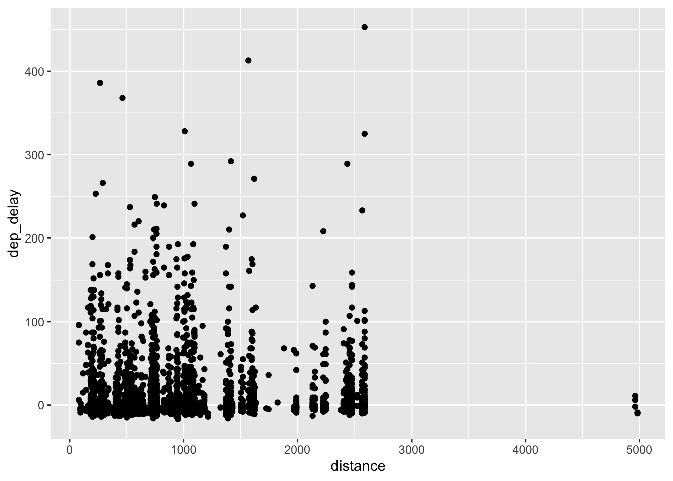
######################
#aesthetic attributes# #color, size, shape
######################
#color by group
ggplot(data, aes(x=distance, y= dep_delay, color=carrier)) +
geom_point()## Warning: Removed 85 rows containing missing values (geom_point).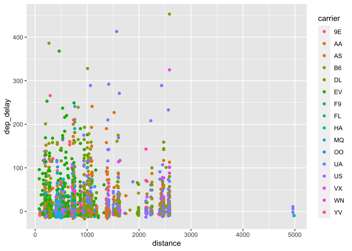
#color of points
ggplot(data, aes(x=distance, y= dep_delay)) +
geom_point(color="blue")## Warning: Removed 85 rows containing missing values (geom_point).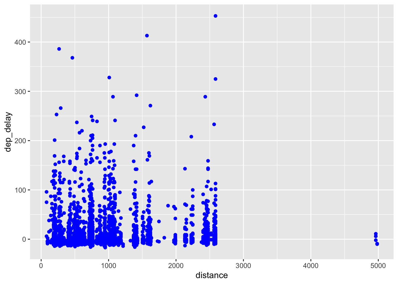
#size
ggplot(data, aes(x=distance, y= dep_delay, size=air_time)) +
geom_point()## Warning: Removed 102 rows containing missing values (geom_point).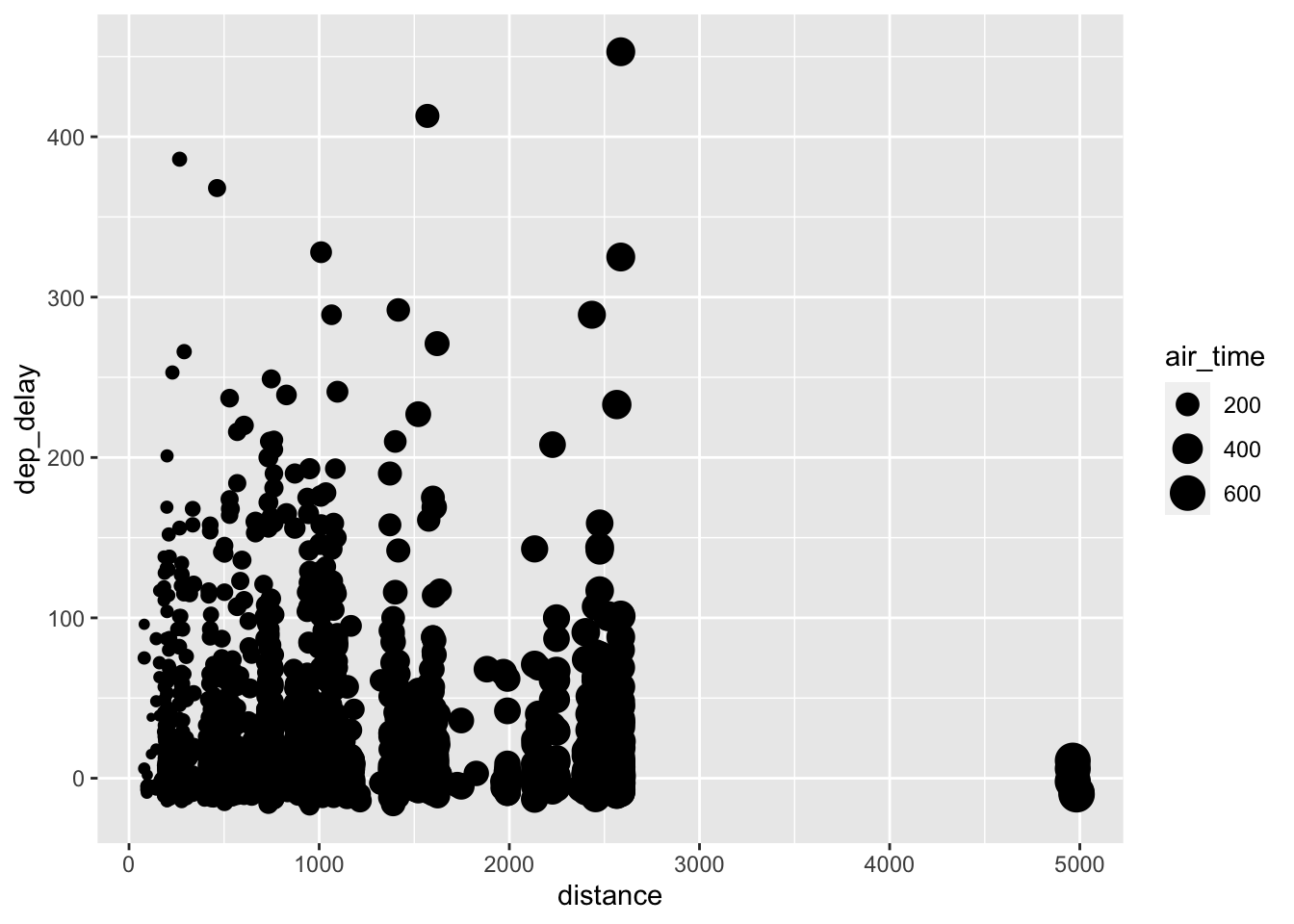
#shape
ggplot(data, aes(x=distance, y= dep_delay, shape = carrier)) +
geom_point()## Warning: The shape palette can deal with a maximum of 6 discrete values because more than 6 becomes difficult to
## discriminate; you have 16. Consider specifying shapes manually if you must have them.## Warning: Removed 1342 rows containing missing values (geom_point).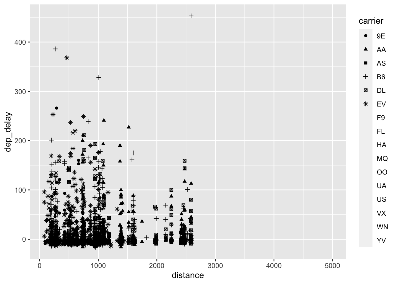
###########
#facetting# for different categories
###########
#facet_wrap
ggplot(data, aes(x=distance, y= dep_delay)) +
geom_point() +
facet_wrap(~carrier)## Warning: Removed 85 rows containing missing values (geom_point).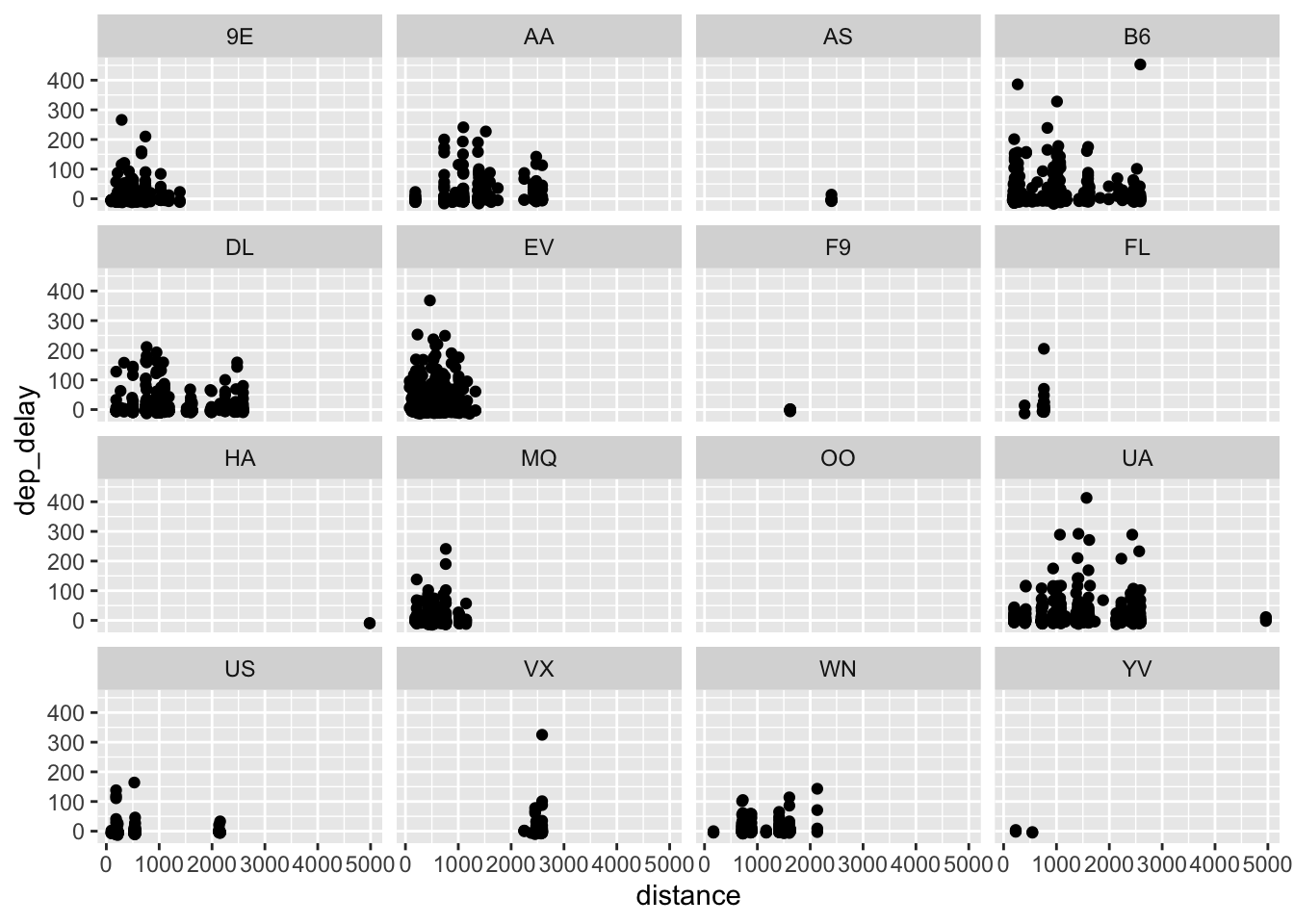
ggplot(data, aes(x=distance, y= dep_delay)) +
  geom_point() +
  facet_wrap(~month)
## Warning: Removed 85 rows containing missing values (geom_point).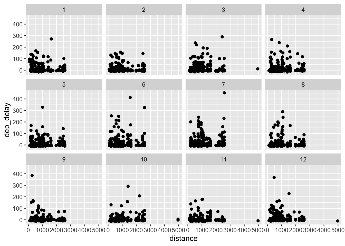
#colnames(data)
#range(data$month)

#facet_grid
ggplot(data, aes(x=distance, y= dep_delay)) +
  geom_point() +
  facet_grid(~carrier)
## Warning: Removed 85 rows containing missing values (geom_point).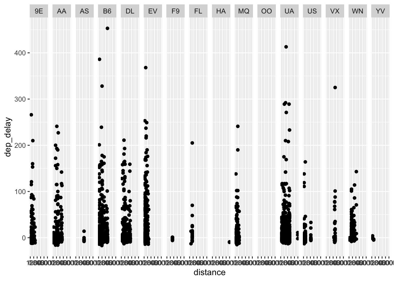
###########
#smoothing# for trend
###########

ggplot(data, aes(x=distance, y= dep_delay)) +
  geom_point() +
  geom_smooth()
## `geom_smooth()` using method = 'gam' and formula 'y ~ s(x, bs = "cs")'## Warning: Removed 85 rows containing non-finite values (stat_smooth).## Warning: Removed 85 rows containing missing values (geom_point).
ggplot(data, aes(x=distance, y= dep_delay)) +
  geom_point() +
  geom_smooth(se=T)
## `geom_smooth()` using method = 'gam' and formula 'y ~ s(x, bs = "cs")'## Warning: Removed 85 rows containing non-finite values (stat_smooth).
## Warning: Removed 85 rows containing missing values (geom_point).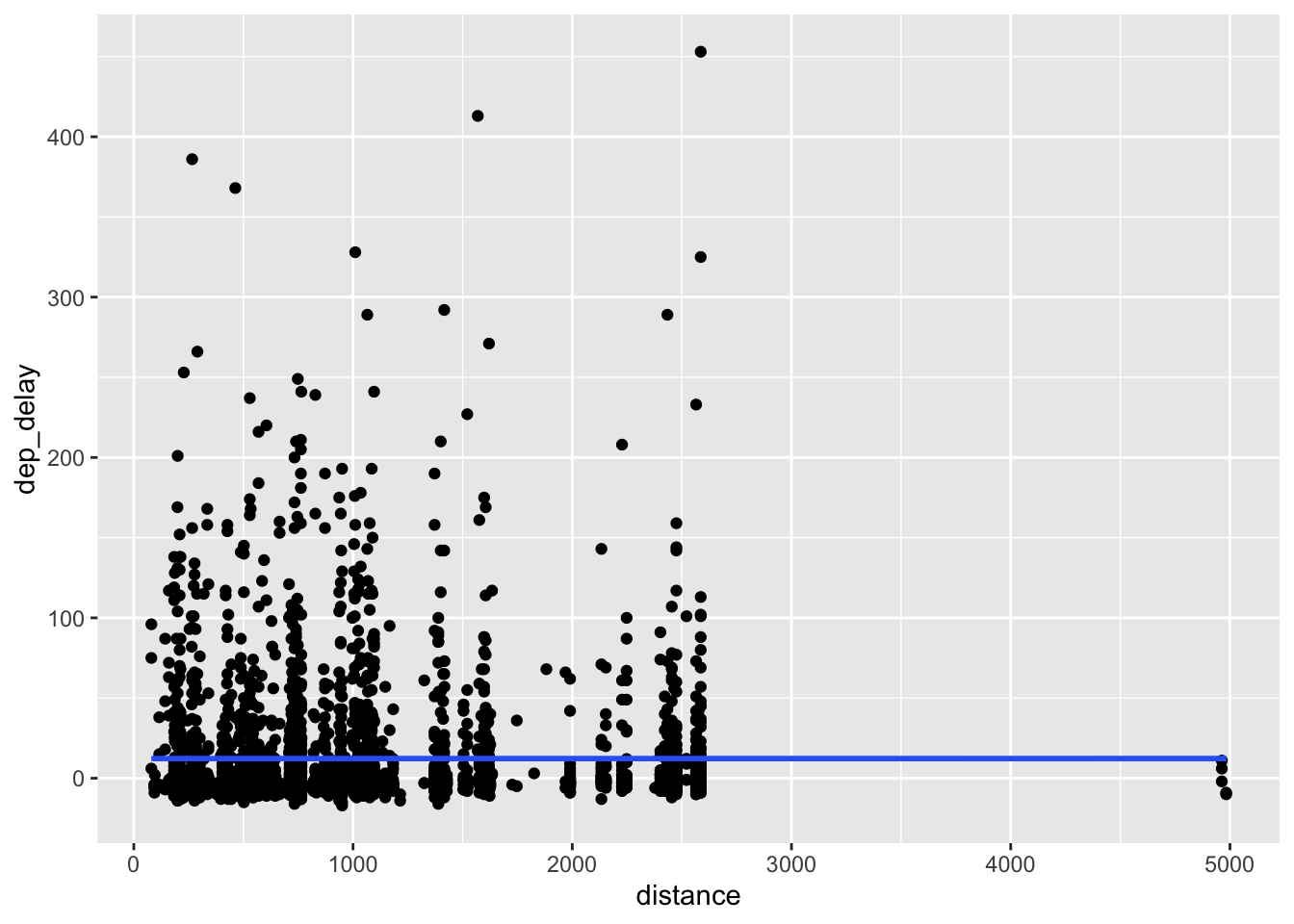
#varying the smooth
data %>%
  filter(distance<3000, dep_delay<400) %>%
  ggplot(aes(x=distance, y= dep_delay)) +
  geom_point() +
  geom_smooth(method="loess", span = 0.1)
## `geom_smooth()` using formula 'y ~ x'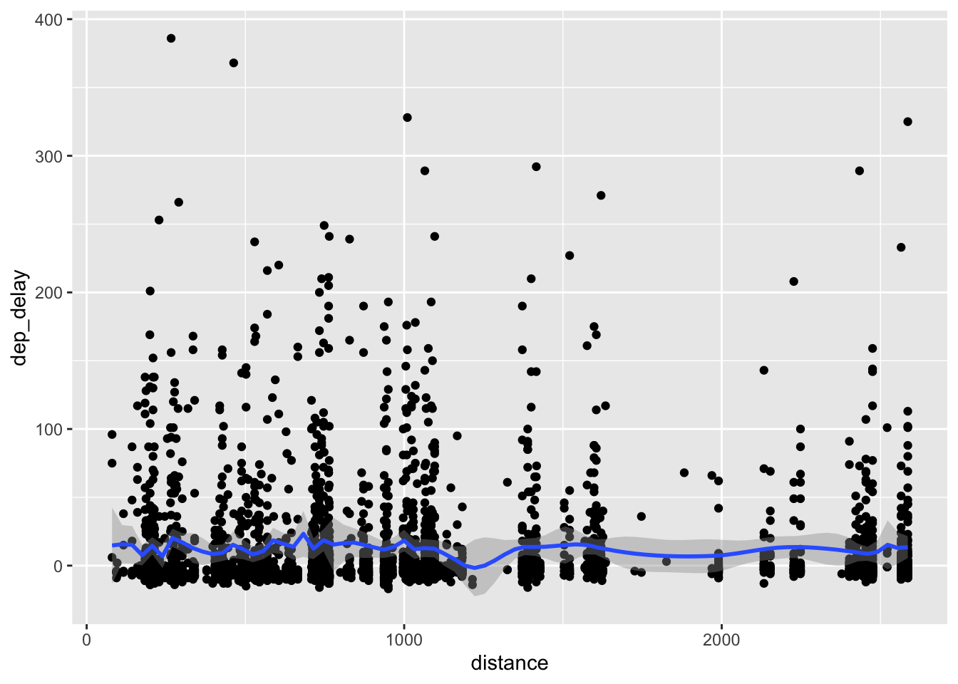
data %>%
  filter(distance<3000) %>%
  ggplot(aes(x=distance, y= dep_delay)) +
  geom_point() +
  geom_smooth(method="loess", span = 1)
## `geom_smooth()` using formula 'y ~ x'## Warning: Removed 85 rows containing non-finite values (stat_smooth).
## Warning: Removed 85 rows containing missing values (geom_point).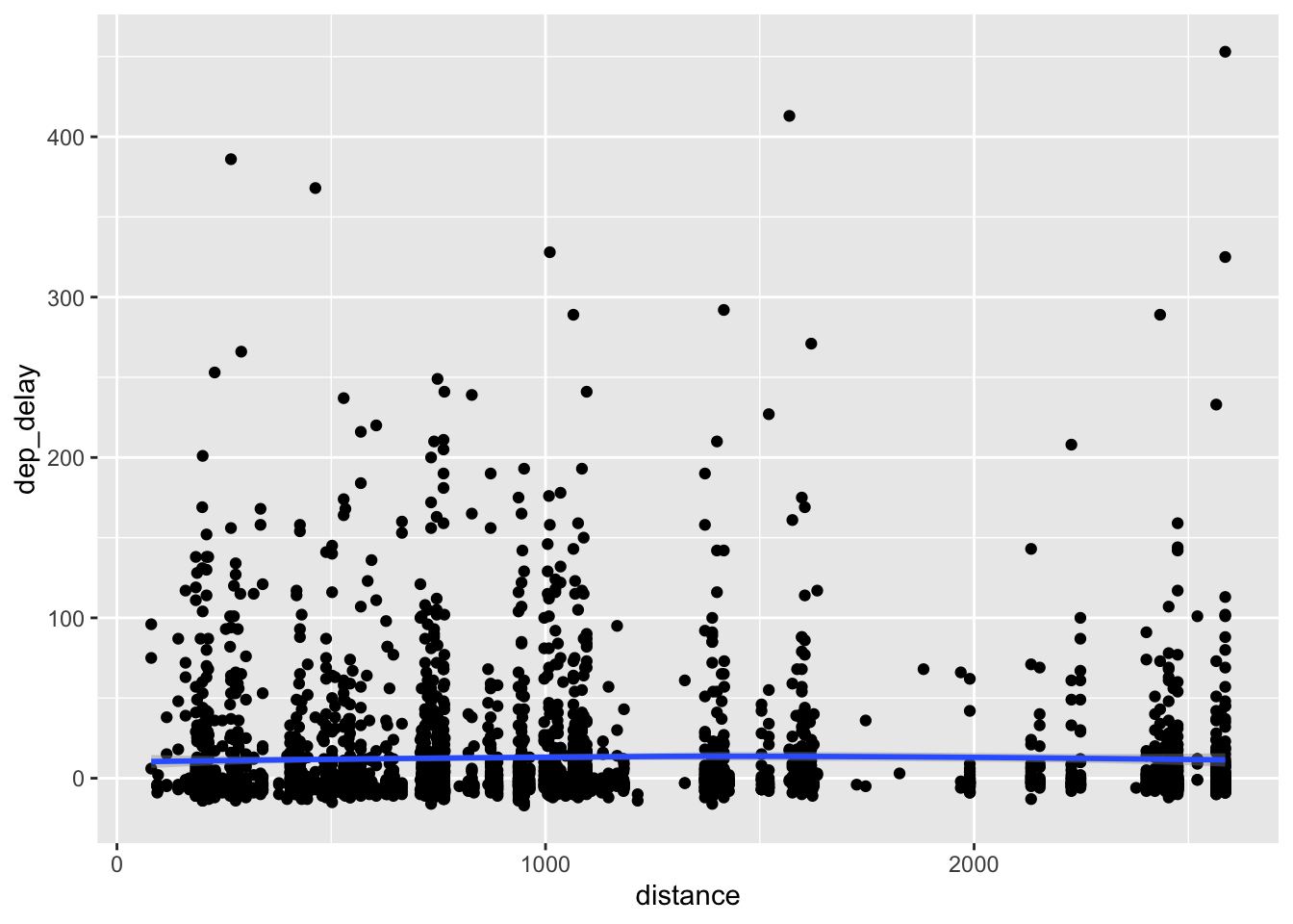
ggplot(data, aes(x=distance, y= dep_delay)) +
  geom_point() +
  geom_smooth(method="loess")
## `geom_smooth()` using formula 'y ~ x'## Warning: Removed 85 rows containing non-finite values (stat_smooth).
## Warning: Removed 85 rows containing missing values (geom_point).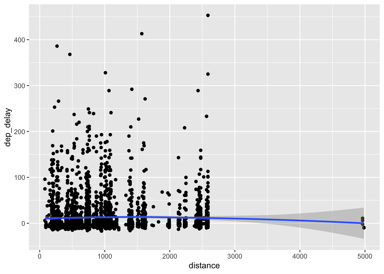
ggplot(data, aes(x=distance, y= dep_delay)) +
  geom_point() +
  geom_smooth(method="lm")
## `geom_smooth()` using formula 'y ~ x'## Warning: Removed 85 rows containing non-finite values (stat_smooth).
## Warning: Removed 85 rows containing missing values (geom_point).
library(mgcv)
ggplot(data, aes(x=distance, y= dep_delay)) +
  geom_point() +
  geom_smooth(method="gam", formula = y ~s(x))
## Warning: Removed 85 rows containing non-finite values (stat_smooth).
## Warning: Removed 85 rows containing missing values (geom_point).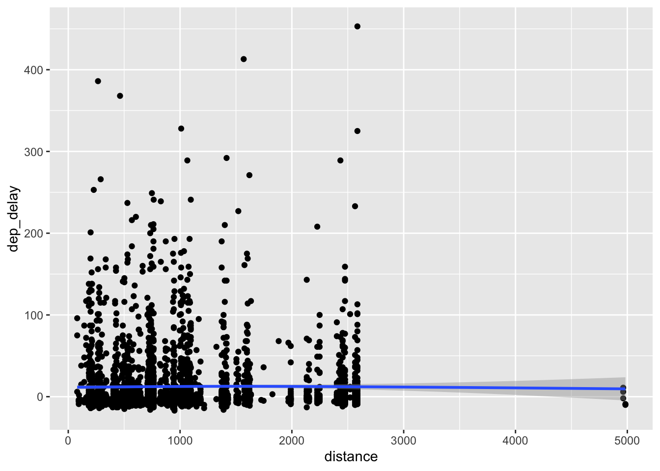
############################
#continuous vs. categorical#
############################

#jitter plot
ggplot(data, aes(x=carrier, y= dep_delay)) +
  geom_jitter()
## Warning: Removed 85 rows containing missing values (geom_point).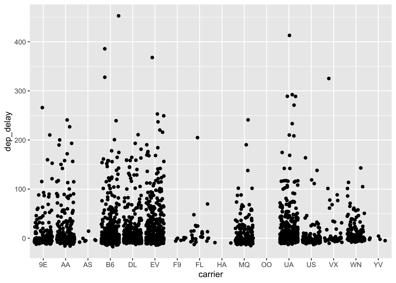
#boxplot
ggplot(data, aes(x=carrier, y= dep_delay)) +
  geom_boxplot()
## Warning: Removed 85 rows containing non-finite values (stat_boxplot).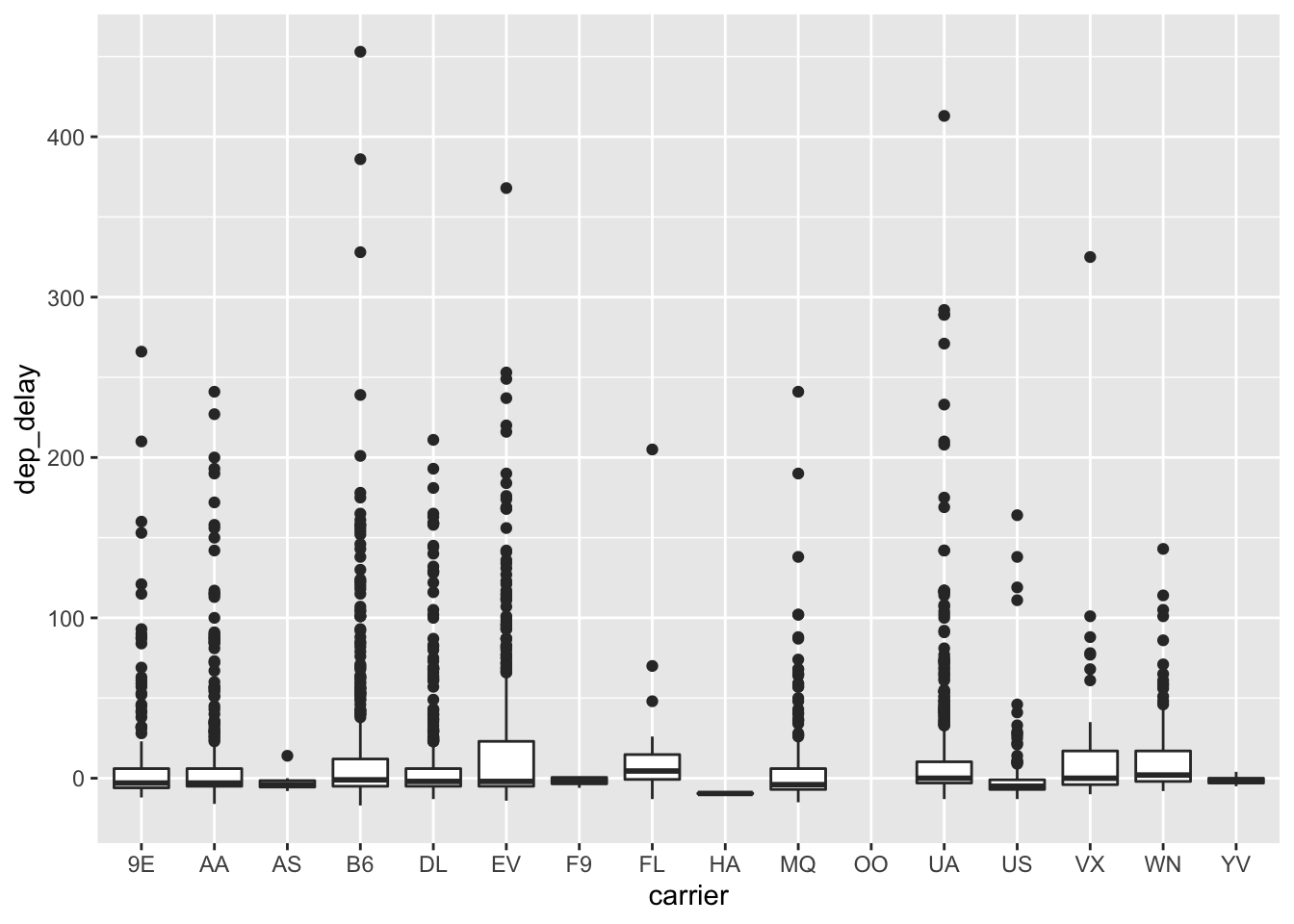
#violin
ggplot(data, aes(x=carrier, y= dep_delay)) +
  geom_violin()
## Warning: Removed 85 rows containing non-finite values (stat_ydensity).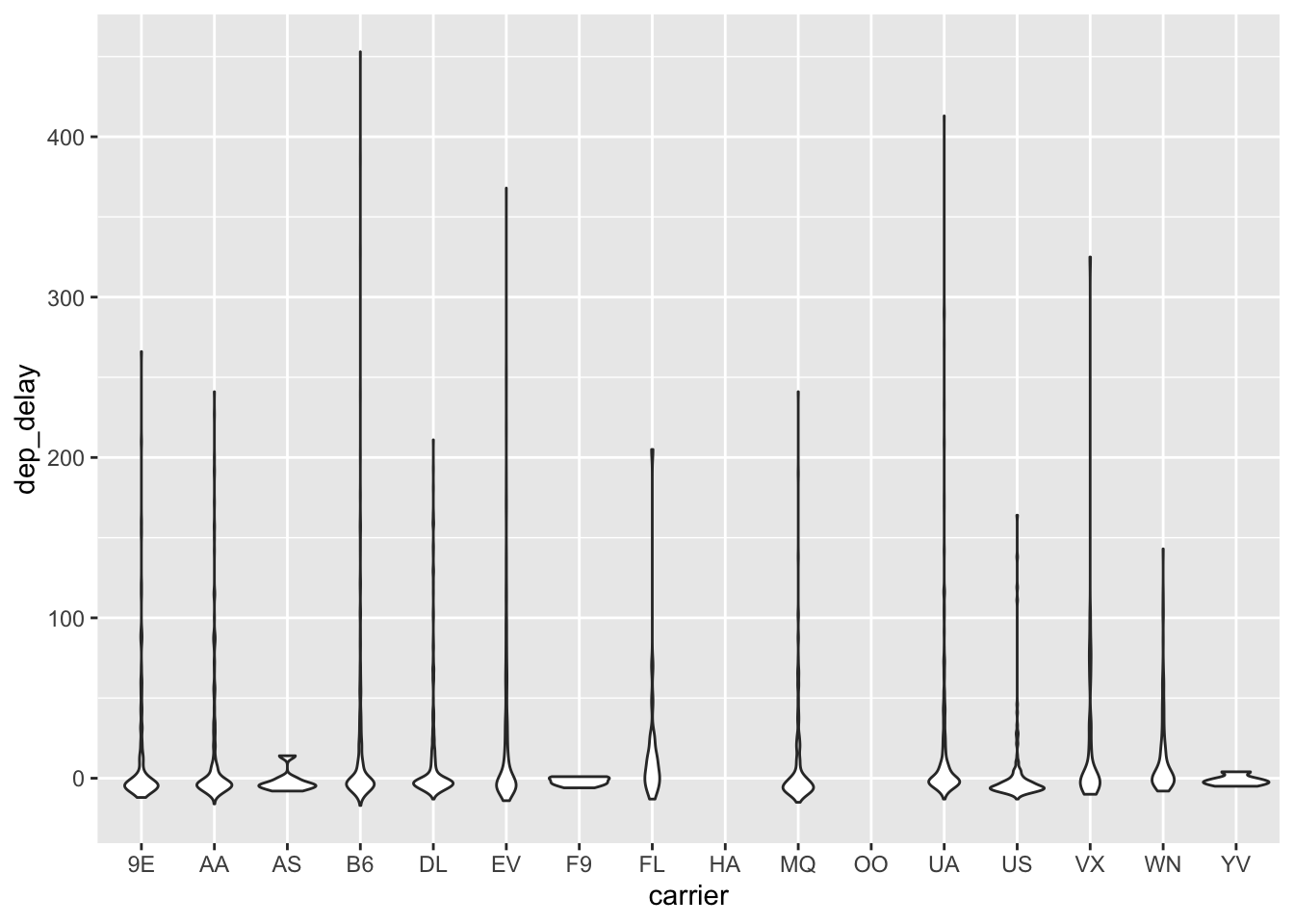
##########################
#continuous distributions#
##########################

#histograms
ggplot(data, aes(dep_delay)) +
  geom_histogram(binwidth=25)
## Warning: Removed 85 rows containing non-finite values (stat_bin).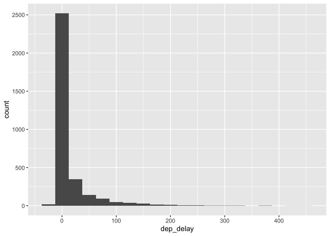
ggplot(data, aes(dep_delay)) +
  geom_histogram(binwidth=1)
## Warning: Removed 85 rows containing non-finite values (stat_bin).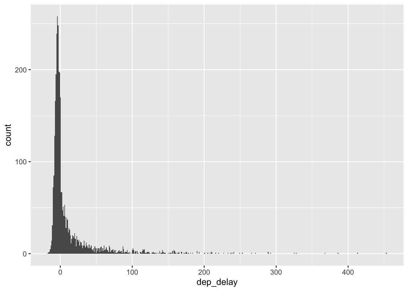
#frequency plots
ggplot(data, aes(dep_delay)) +
  geom_freqpoly(binwidth=25)
## Warning: Removed 85 rows containing non-finite values (stat_bin).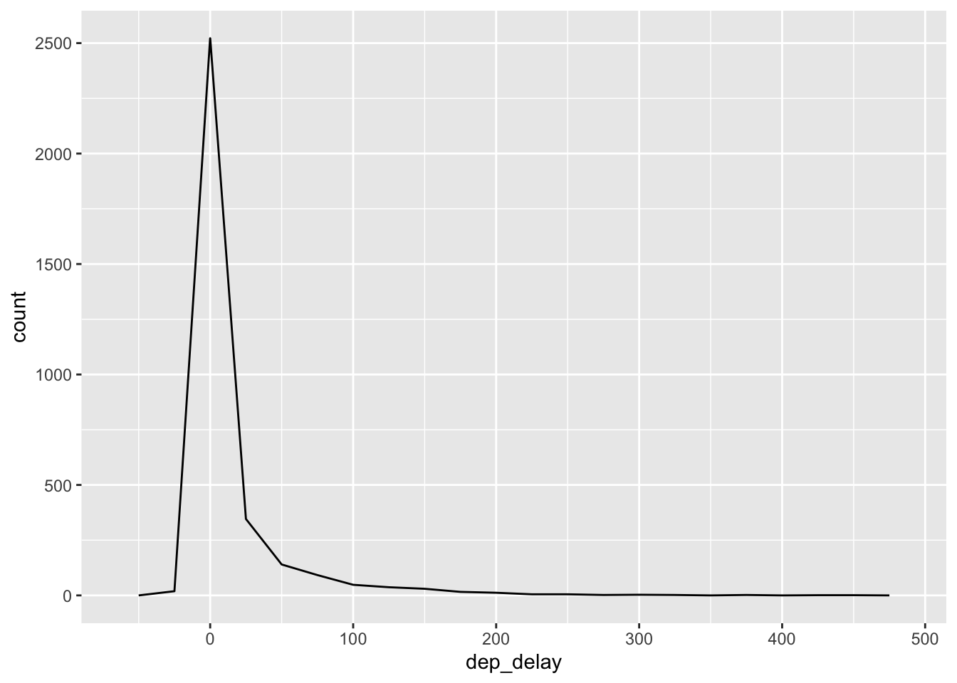
ggplot(data, aes(dep_delay)) +
  geom_freqpoly(binwidth=1)
## Warning: Removed 85 rows containing non-finite values (stat_bin).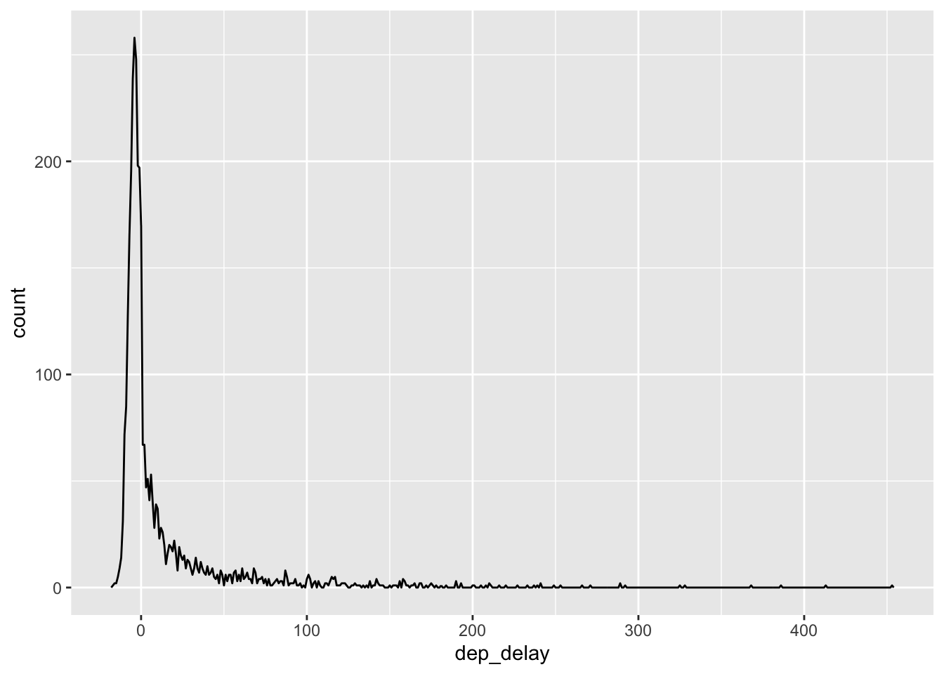
#adding aesthetics
ggplot(data, aes(dep_delay, color=carrier)) +
  geom_freqpoly(binwidth=25)
## Warning: Removed 85 rows containing non-finite values (stat_bin).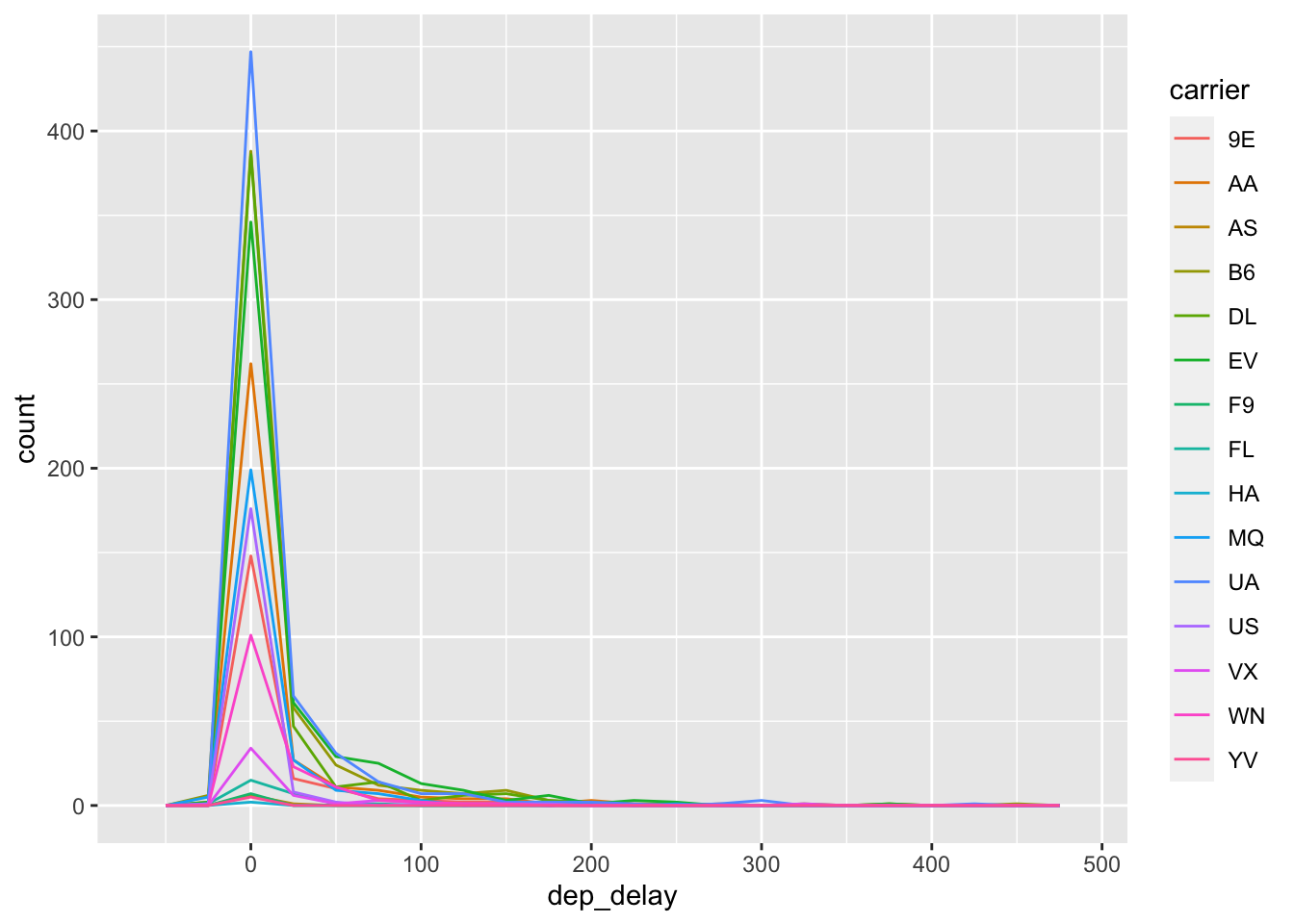
ggplot(data, aes( dep_delay, fill = carrier)) +
  geom_histogram(binwidth=20) +
  facet_wrap(~carrier)
## Warning: Removed 85 rows containing non-finite values (stat_bin).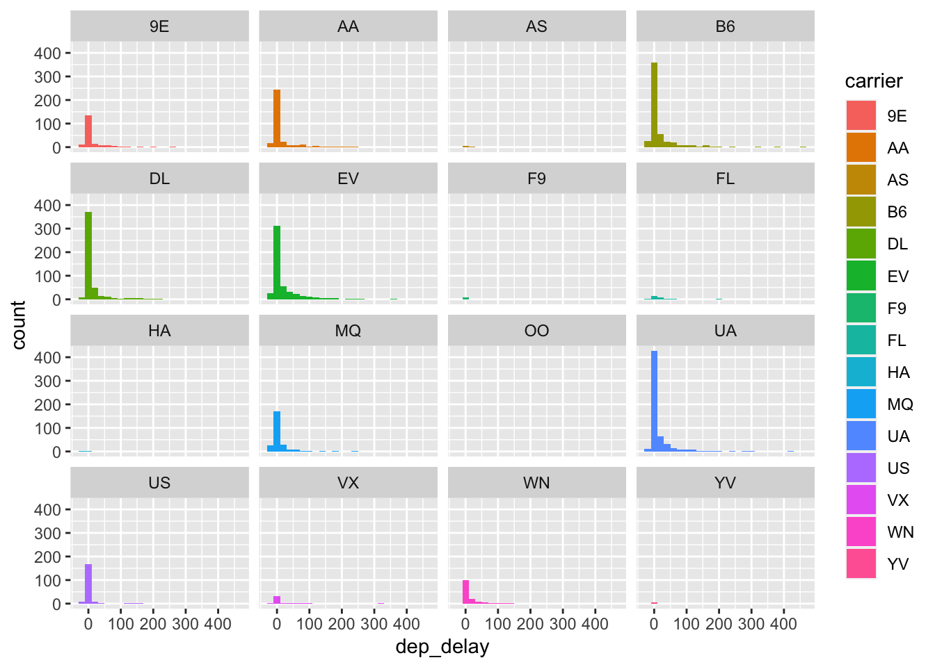
##############
#extra graphs#
##############

#bar charts
ggplot(data, aes(carrier))+
  geom_bar()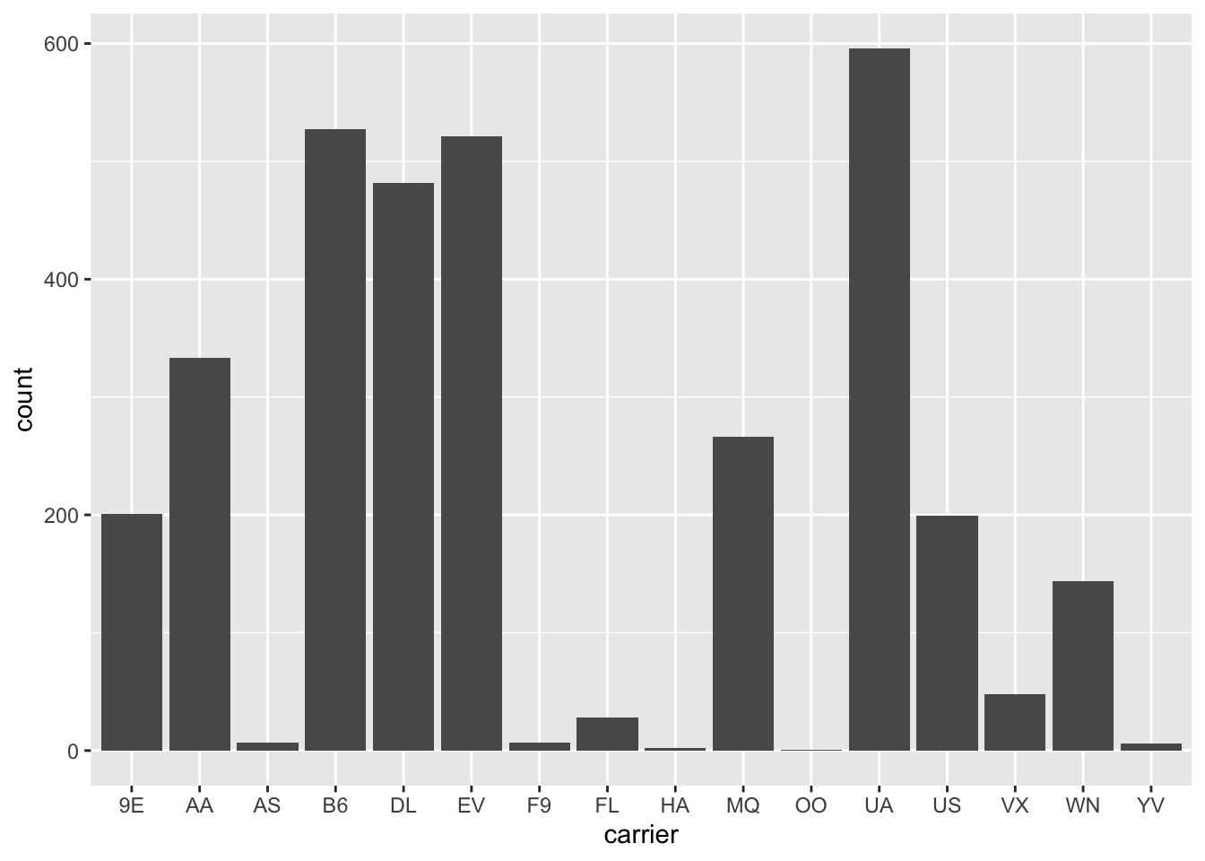
#line and path plots
ggplot(data, aes(x=dep_delay, y=distance/air_time*60))+
  #geom_point()+
  geom_smooth(method = "lm")+
  geom_line()
## `geom_smooth()` using formula 'y ~ x'## Warning: Removed 102 rows containing non-finite values (stat_smooth).## Warning: Removed 85 row(s) containing missing values (geom_path).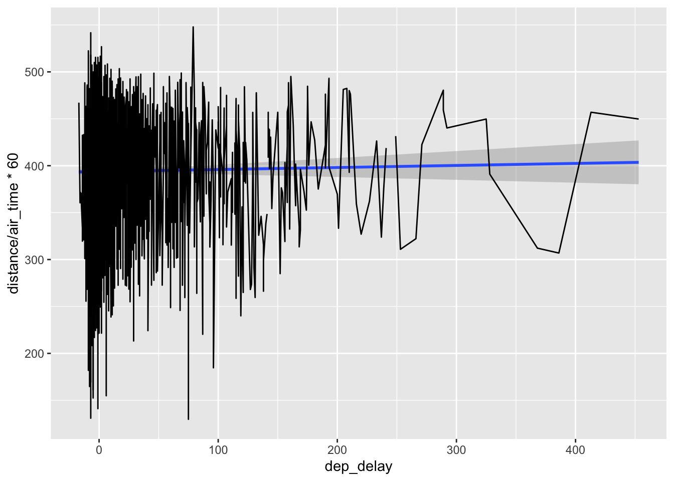
##########
#labeling#
##########

#labeling the axes
ggplot(data, aes(dep_delay, distance/air_time*60)) +
  geom_point(alpha = 1 / 3) +
  xlab("Departure Delay (minutes)") +
  ylab("Speed (MPH)")
## Warning: Removed 102 rows containing missing values (geom_point).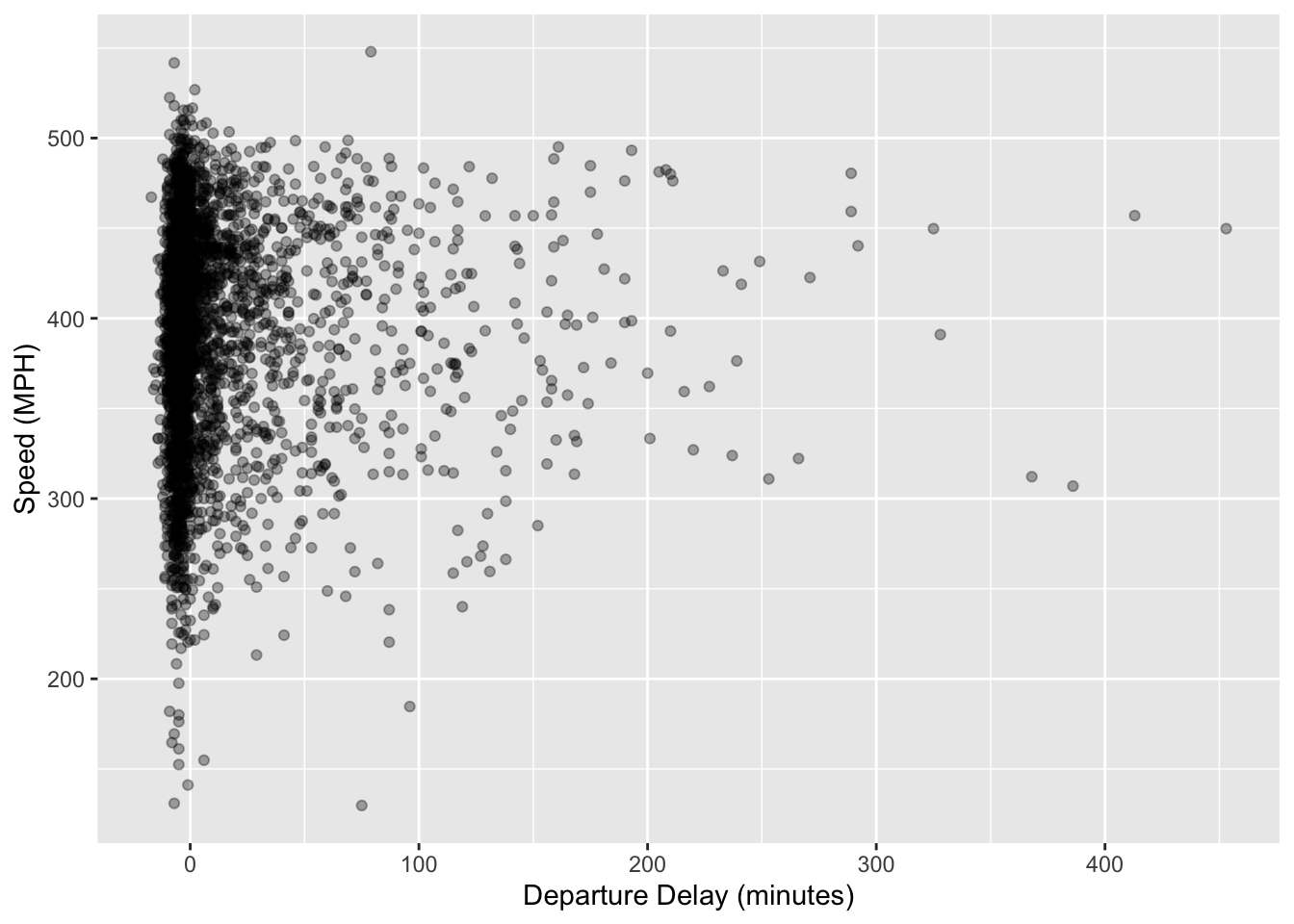
#font familites
df <- data.frame(x = 1:3, y = 3:1, family = c("sans", "serif", "mono"))
ggplot(df, aes(x, y)) +
  geom_text(aes(label = family, family = family))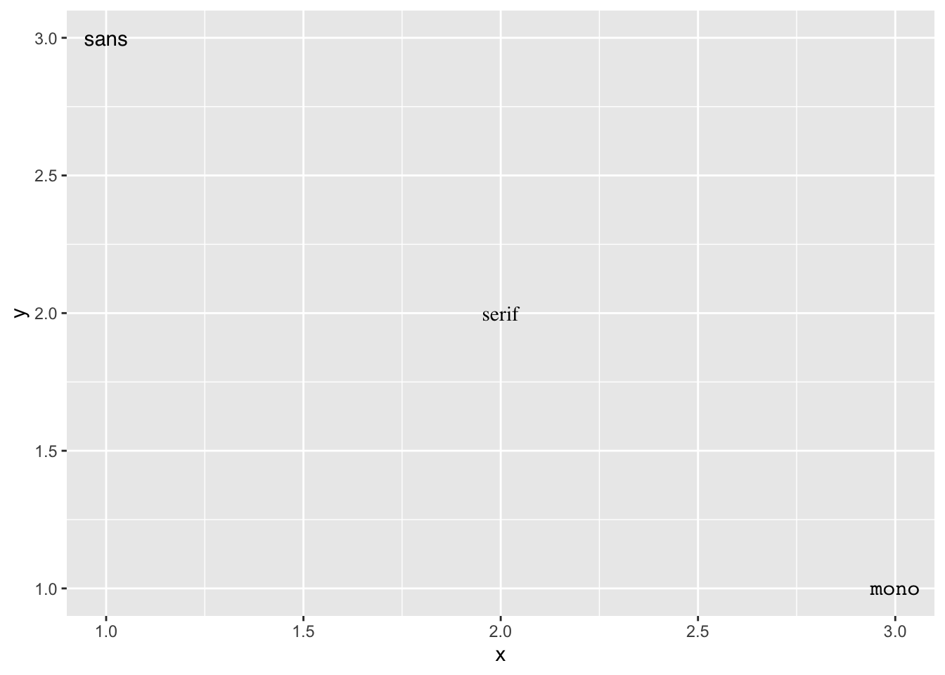
#font face styles
df <- data.frame(x = 1:3, y = 3:1, face = c("plain", "bold", "italic"))
ggplot(df, aes(x, y)) +
  geom_text(aes(label = face, fontface = face))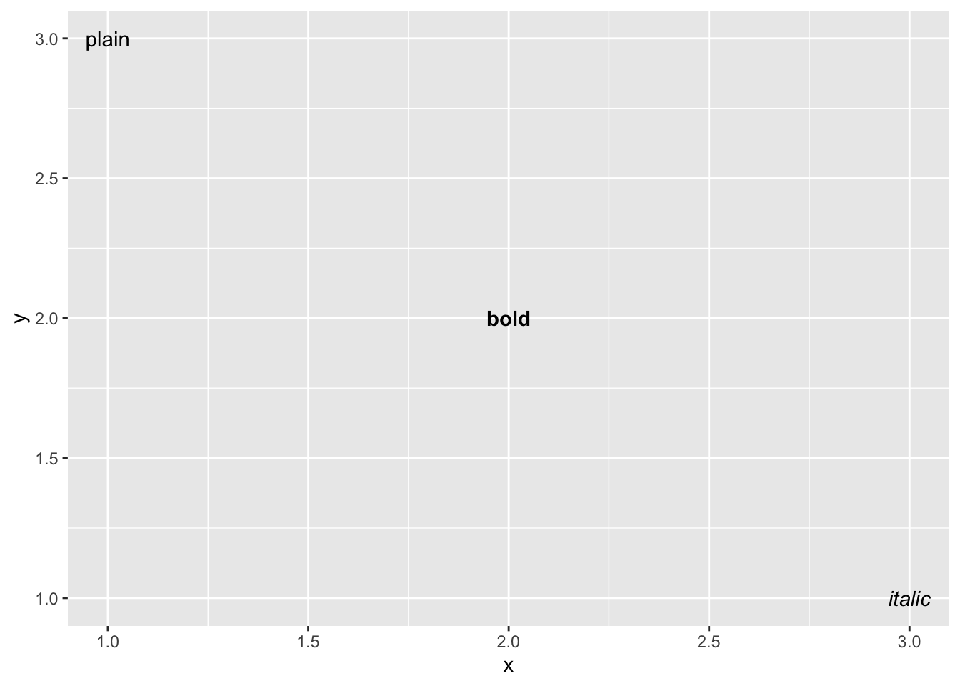
#nudge to label existing points
df <- data.frame(trt = c("a", "b", "c"), resp = c(1.2, 3.4, 2.5))
ggplot(df, aes(resp, trt)) +
  geom_point() +
  geom_text(aes(label = paste0("(", resp, ")")), nudge_y = -0.25) +
  xlim(1, 3.6)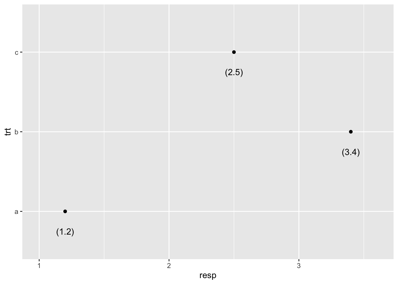
#labels rather than a legend
library(directlabels)
library(gridExtra)
mpg
## # A tibble: 234 x 11
## manufacturer model displ year cyl trans drv cty hwy fl class
## <chr> <chr> <dbl> <int> <int> <chr> <chr> <int> <int> <chr> <chr>
## 1 audi a4 1.8 1999 4 auto(l5) f 18 29 p compact
## 2 audi a4 1.8 1999 4 manual(m5) f 21 29 p compact
## 3 audi a4 2 2008 4 manual(m6) f 20 31 p compact
## 4 audi a4 2 2008 4 auto(av) f 21 30 p compact
## 5 audi a4 2.8 1999 6 auto(l5) f 16 26 p compact
## 6 audi a4 2.8 1999 6 manual(m5) f 18 26 p compact
## 7 audi a4 3.1 2008 6 auto(av) f 18 27 p compact
## 8 audi a4 quattro 1.8 1999 4 manual(m5) 4 18 26 p compact
## 9 audi a4 quattro 1.8 1999 4 auto(l5) 4 16 25 p compact
## 10 audi a4 quattro 2 2008 4 manual(m6) 4 20 28 p compact
## # … with 224 more rowsp1 <- ggplot(mpg, aes(displ, hwy, colour = class)) +
geom_point()
mpg$class## [1] "compact" "compact" "compact" "compact" "compact" "compact" "compact" "compact" "compact"
## [10] "compact" "compact" "compact" "compact" "compact" "compact" "midsize" "midsize" "midsize"
## [19] "suv" "suv" "suv" "suv" "suv" "2seater" "2seater" "2seater" "2seater"
## [28] "2seater" "suv" "suv" "suv" "suv" "midsize" "midsize" "midsize" "midsize"
## [37] "midsize" "minivan" "minivan" "minivan" "minivan" "minivan" "minivan" "minivan" "minivan"
## [46] "minivan" "minivan" "minivan" "pickup" "pickup" "pickup" "pickup" "pickup" "pickup"
## [55] "pickup" "pickup" "pickup" "suv" "suv" "suv" "suv" "suv" "suv"
## [64] "suv" "pickup" "pickup" "pickup" "pickup" "pickup" "pickup" "pickup" "pickup"
## [73] "pickup" "pickup" "suv" "suv" "suv" "suv" "suv" "suv" "suv"
## [82] "suv" "suv" "pickup" "pickup" "pickup" "pickup" "pickup" "pickup" "pickup"
## [91] "subcompact" "subcompact" "subcompact" "subcompact" "subcompact" "subcompact" "subcompact" "subcompact" "subcompact"
## [100] "subcompact" "subcompact" "subcompact" "subcompact" "subcompact" "subcompact" "subcompact" "subcompact" "subcompact"
## [109] "midsize" "midsize" "midsize" "midsize" "midsize" "midsize" "midsize" "subcompact" "subcompact"
## [118] "subcompact" "subcompact" "subcompact" "subcompact" "subcompact" "suv" "suv" "suv" "suv"
## [127] "suv" "suv" "suv" "suv" "suv" "suv" "suv" "suv" "suv"
## [136] "suv" "suv" "suv" "suv" "suv" "suv" "compact" "compact" "midsize"
## [145] "midsize" "midsize" "midsize" "midsize" "midsize" "midsize" "suv" "suv" "suv"
## [154] "suv" "midsize" "midsize" "midsize" "midsize" "midsize" "suv" "suv" "suv"
## [163] "suv" "suv" "suv" "subcompact" "subcompact" "subcompact" "subcompact" "compact" "compact"
## [172] "compact" "compact" "suv" "suv" "suv" "suv" "suv" "suv" "midsize"
## [181] "midsize" "midsize" "midsize" "midsize" "midsize" "midsize" "compact" "compact" "compact"
## [190] "compact" "compact" "compact" "compact" "compact" "compact" "compact" "compact" "compact"
## [199] "suv" "suv" "pickup" "pickup" "pickup" "pickup" "pickup" "pickup" "pickup"
## [208] "compact" "compact" "compact" "compact" "compact" "compact" "compact" "compact" "compact"
## [217] "compact" "compact" "compact" "compact" "compact" "subcompact" "subcompact" "subcompact" "subcompact"
## [226] "subcompact" "subcompact" "midsize" "midsize" "midsize" "midsize" "midsize" "midsize" "midsize"p1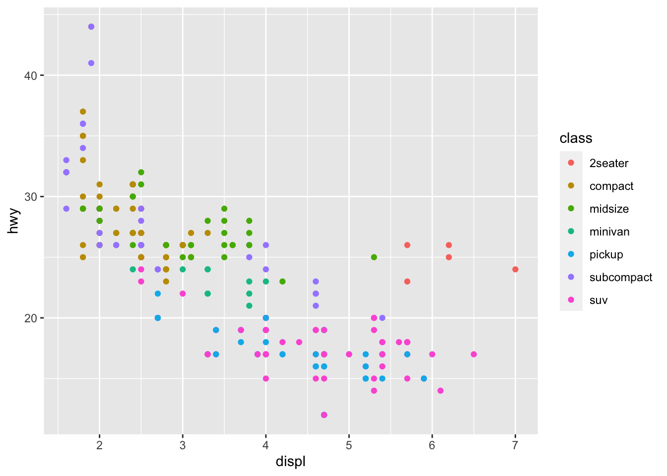
p2 <- ggplot(mpg, aes(displ, hwy, colour = class)) +
  geom_point(show.legend = FALSE) +
  geom_dl(aes(label = class), method = "smart.grid")
p2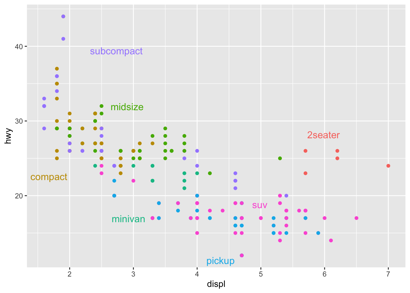
grid.arrange(p1, p2, ncol=2)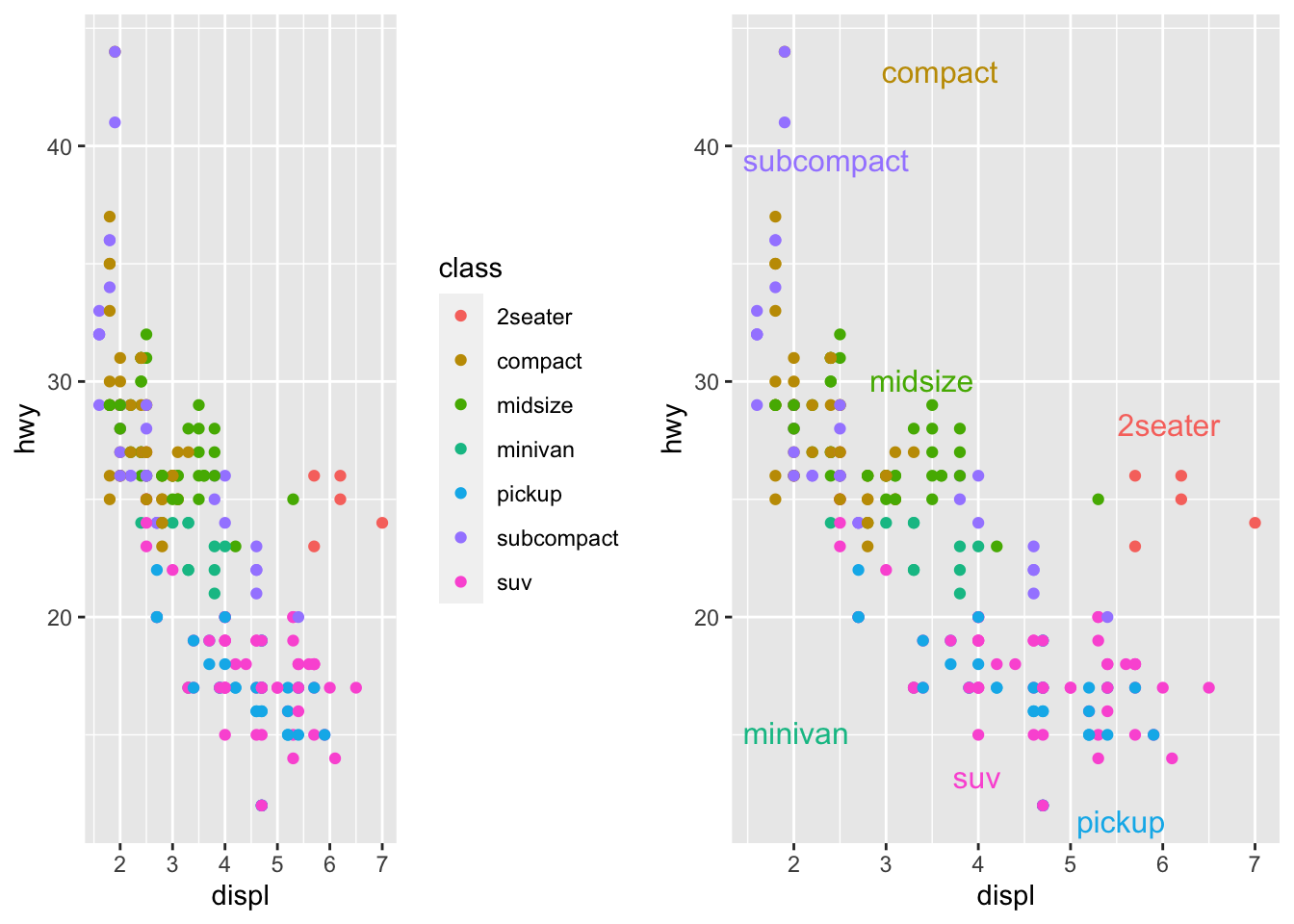
####################
#constructing plots#
####################
library(gridExtra)
p1<-ggplot(data, aes(dep_delay, arr_delay, colour = carrier)) +
  geom_point()
p2<-ggplot(data, aes(dep_delay, arr_delay)) +
  geom_point(aes(colour = carrier))
p3<-ggplot(data, aes(dep_delay)) +
  geom_point(aes(y = arr_delay, colour = carrier))
p4<-ggplot(data) +
  geom_point(aes(dep_delay, arr_delay, colour = carrier))
grid.arrange(p1, p2, p3, p4, ncol=2)
## Warning: Removed 102 rows containing missing values (geom_point).## Warning: Removed 102 rows containing missing values (geom_point).
## Warning: Removed 102 rows containing missing values (geom_point).
## Warning: Removed 102 rows containing missing values (geom_point).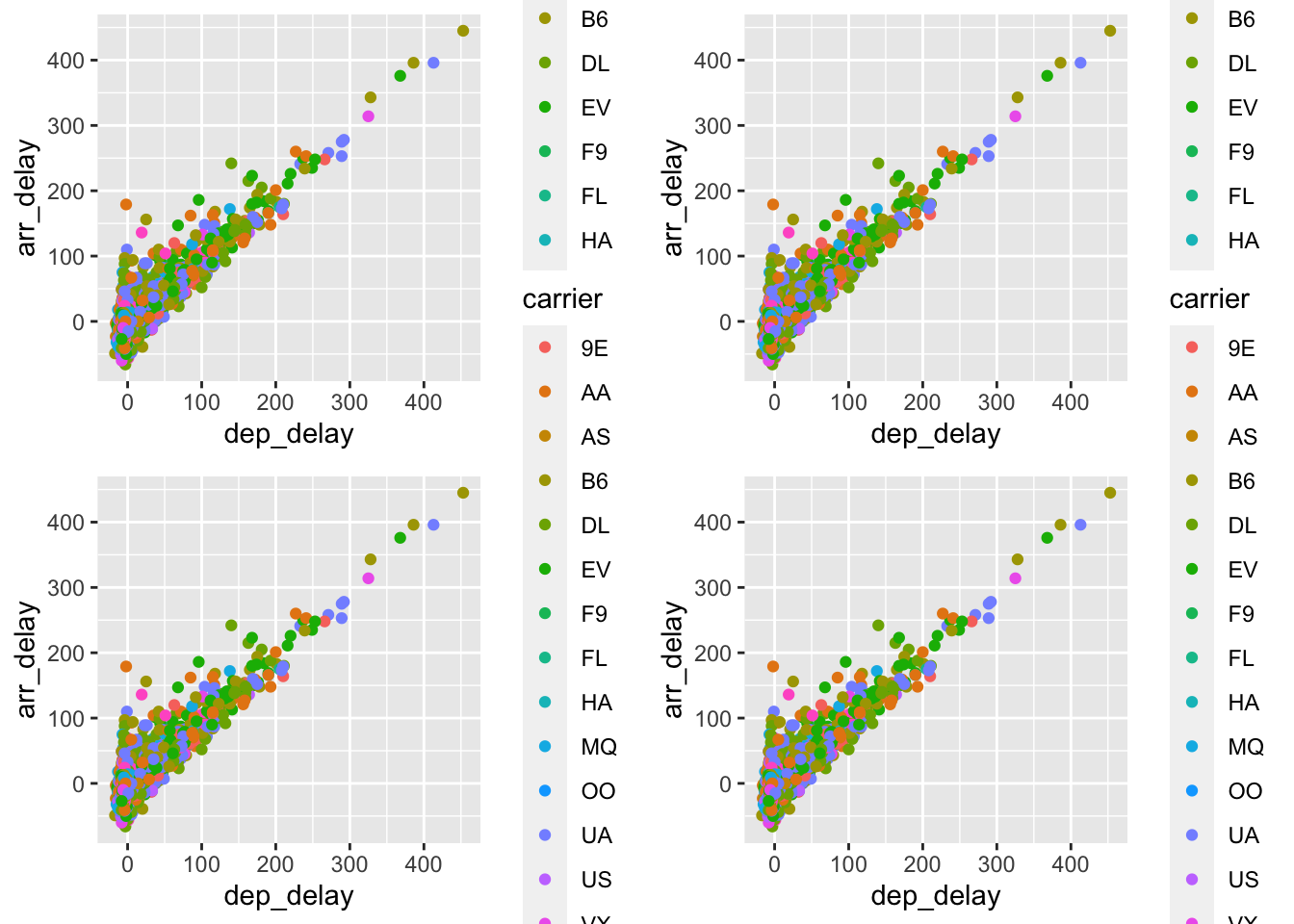
library(gridExtra)
p1 = ggplot(data, aes(dep_delay, arr_delay, colour = carrier)) +
  geom_point() +
  geom_smooth(method = "lm", se = FALSE) +
  theme(legend.position = "none")

p2 = ggplot(data, aes(dep_delay, arr_delay)) +
  geom_point(aes(colour = carrier)) +
  geom_smooth(method = "lm", se = FALSE) +
  theme(legend.position = "none")

grid.arrange(p1,p2, ncol=2)
## `geom_smooth()` using formula 'y ~ x'## Warning: Removed 102 rows containing non-finite values (stat_smooth).
## Warning: Removed 102 rows containing missing values (geom_point).## `geom_smooth()` using formula 'y ~ x'## Warning: Removed 102 rows containing non-finite values (stat_smooth).
## Warning: Removed 102 rows containing missing values (geom_point).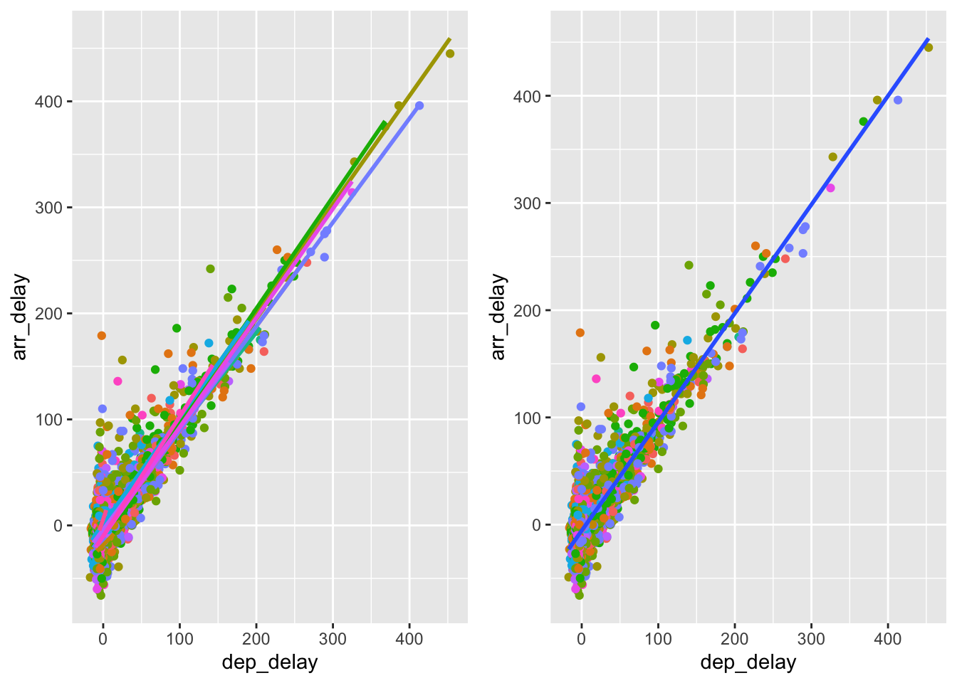
#settings vs. mappings
p1 = ggplot(data, aes(dep_delay, arr_delay)) +
  geom_point(color = "darkblue")
p2 = ggplot(data, aes(dep_delay, arr_delay)) +
  geom_point(aes(color="newvar"))
grid.arrange(p1,p2, ncol=2)
## Warning: Removed 102 rows containing missing values (geom_point).
## Warning: Removed 102 rows containing missing values (geom_point).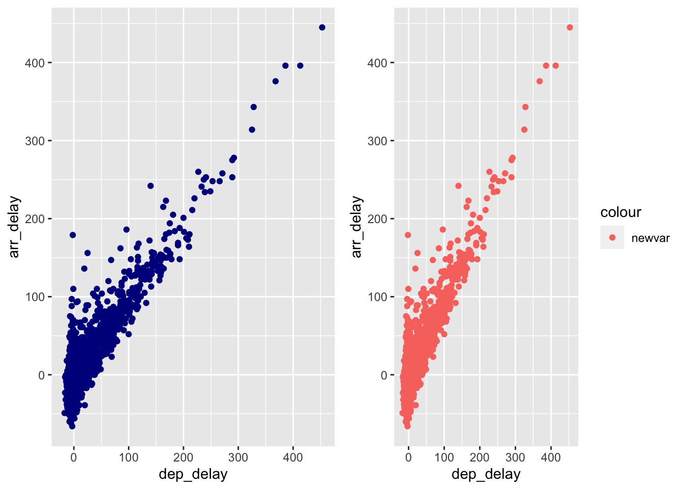
#override
ggplot(data, aes(dep_delay, arr_delay))+
  geom_point(aes(color="darkblue")) +
  scale_color_identity()
## Warning: Removed 102 rows containing missing values (geom_point).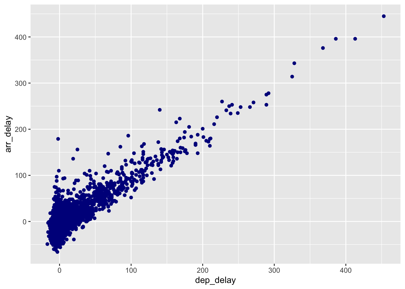
ggplot(data, aes(dep_delay, arr_delay)) +
  geom_point() +
  geom_smooth(aes(color="lm"), method="lm", se=F) +
  geom_smooth(aes(color="loess"), method="loess", se=F) +
  labs(color = "Method")
## `geom_smooth()` using formula 'y ~ x'## Warning: Removed 102 rows containing non-finite values (stat_smooth).## `geom_smooth()` using formula 'y ~ x'## Warning: Removed 102 rows containing non-finite values (stat_smooth).
## Warning: Removed 102 rows containing missing values (geom_point).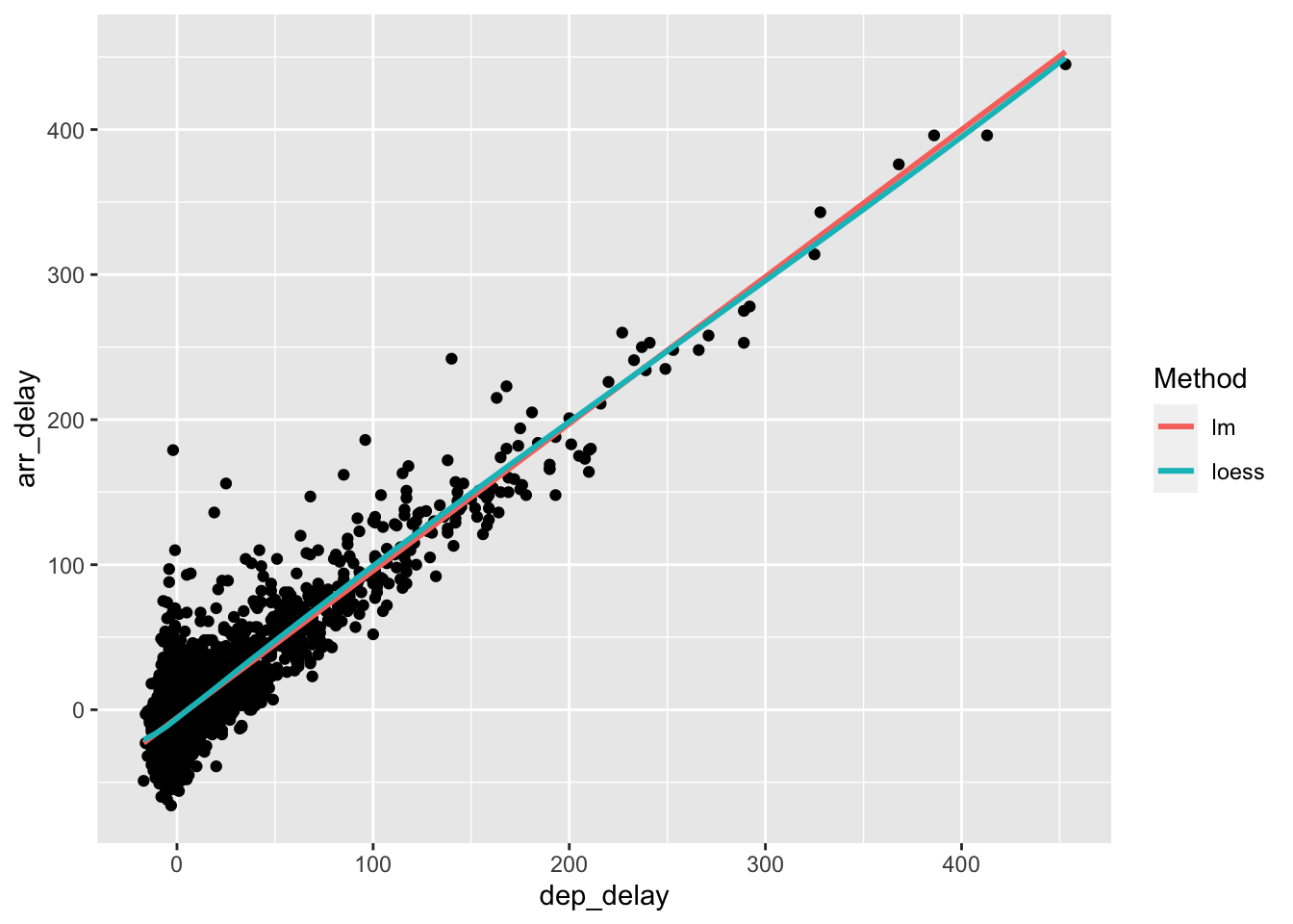
#statistical transforms
ggplot(data, aes(carrier, dep_delay)) +
  geom_point() +
  stat_summary(geom = "point", fun = "median", color = "red", size = 3)
## Warning: Removed 85 rows containing non-finite values (stat_summary).## Warning: Removed 85 rows containing missing values (geom_point).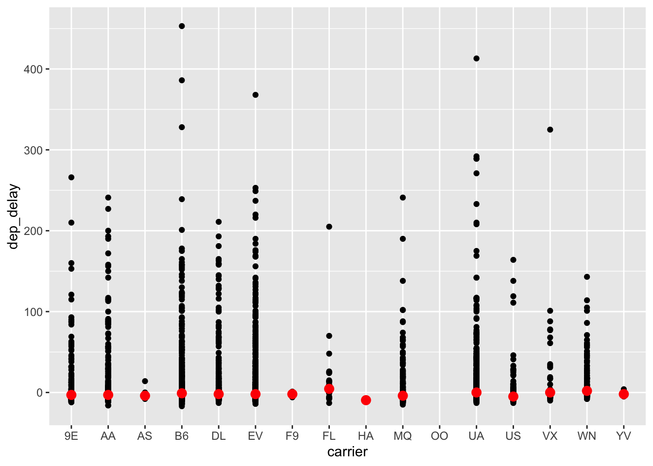
ggplot(data, aes(carrier, dep_delay)) +
  geom_point()+
  geom_point(stat = "summary", fun = "median", color = "red", size = 3)
## Warning: Removed 85 rows containing non-finite values (stat_summary).
## Warning: Removed 85 rows containing missing values (geom_point).
#position adjustments
head(diamonds)
## # A tibble: 6 x 10
## carat cut color clarity depth table price x y z
## <dbl> <ord> <ord> <ord> <dbl> <dbl> <int> <dbl> <dbl> <dbl>
## 1 0.23 Ideal E SI2 61.5 55 326 3.95 3.98 2.43
## 2 0.21 Premium E SI1 59.8 61 326 3.89 3.84 2.31
## 3 0.23 Good E VS1 56.9 65 327 4.05 4.07 2.31
## 4 0.290 Premium I VS2 62.4 58 334 4.2 4.23 2.63
## 5 0.31 Good J SI2 63.3 58 335 4.34 4.35 2.75
## 6 0.24 Very Good J VVS2 62.8 57 336 3.94 3.96 2.48dplot <- ggplot(diamonds, aes(color, fill = cut)) +
xlab(NULL) + ylab(NULL) + theme(legend.position = "none")
dplot
# position stack is the default for bars, so geom_bar()
# is equivalent to geom_bar(position = "stack").
p1 = dplot + geom_bar()
p1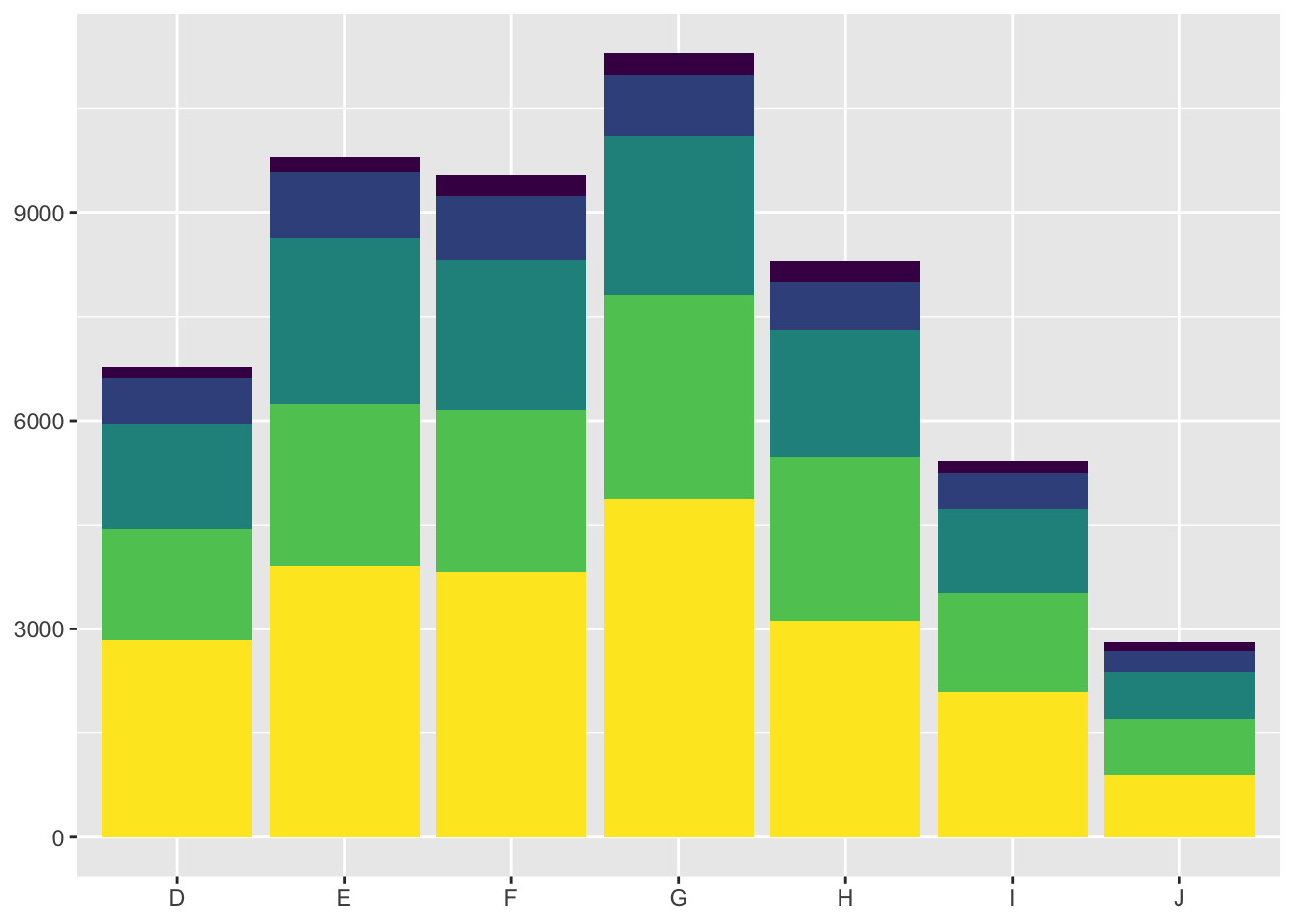
p2 = dplot + geom_bar(position = "fill")
p2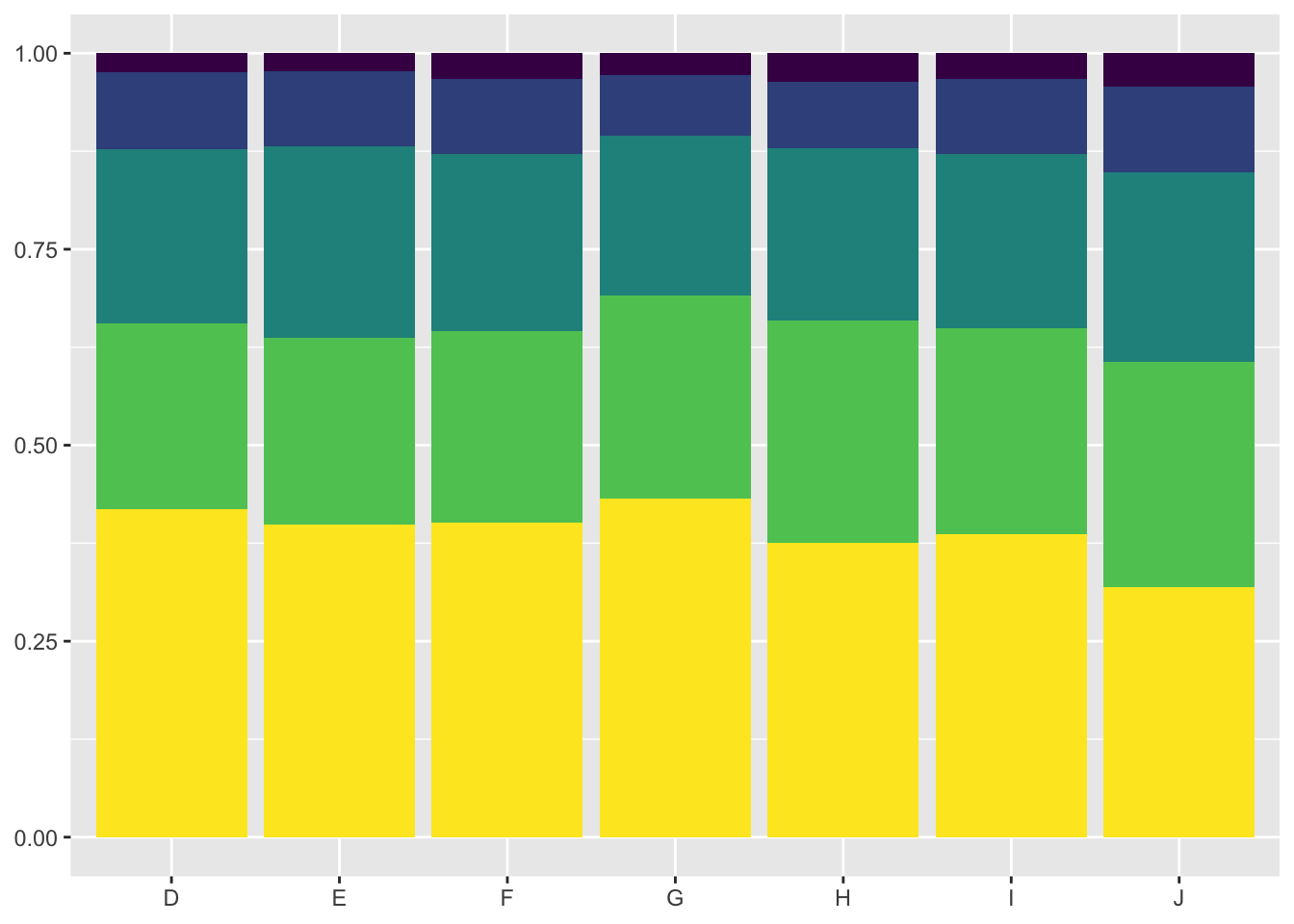
p3 = dplot + geom_bar(position = "dodge")
p3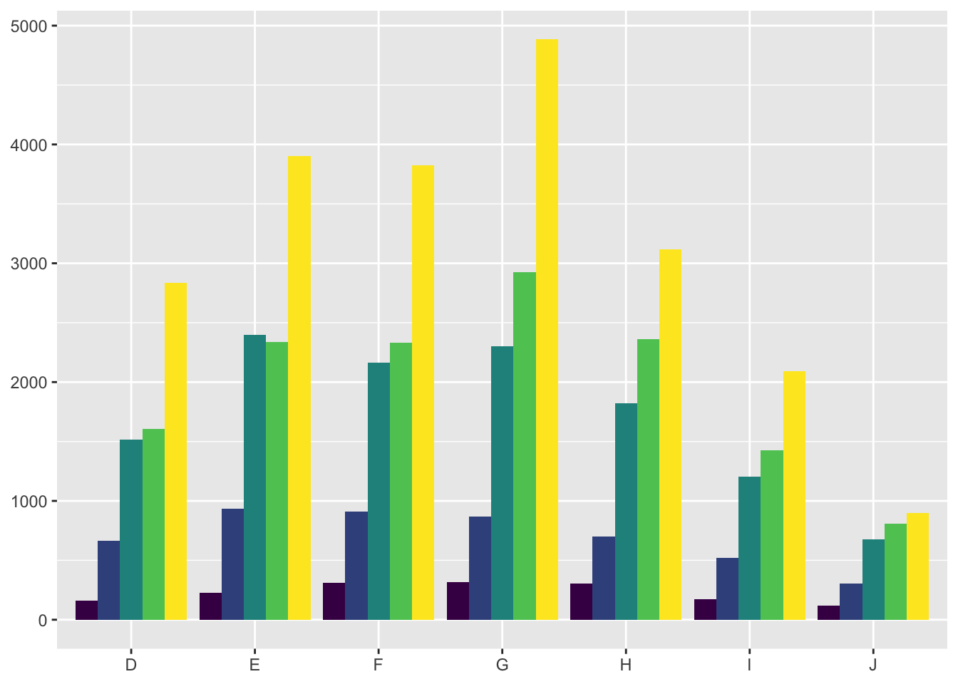
grid.arrange(p1,p2,p3, ncol=3)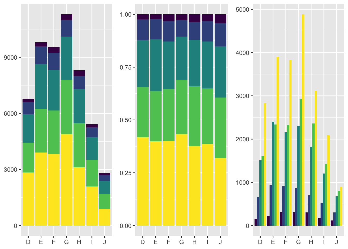
############################################
#modifying axes and scales axes and legends#
############################################

#scale title
df <- data.frame(x = 1:2, y = 1, z = "a")
p <- ggplot(df, aes(x, y)) + geom_point()
p1 = p + scale_x_continuous("X axis")
p2 = p + scale_x_continuous(quote(a + mathematical ^ expression))
grid.arrange(p1,p2, ncol=2)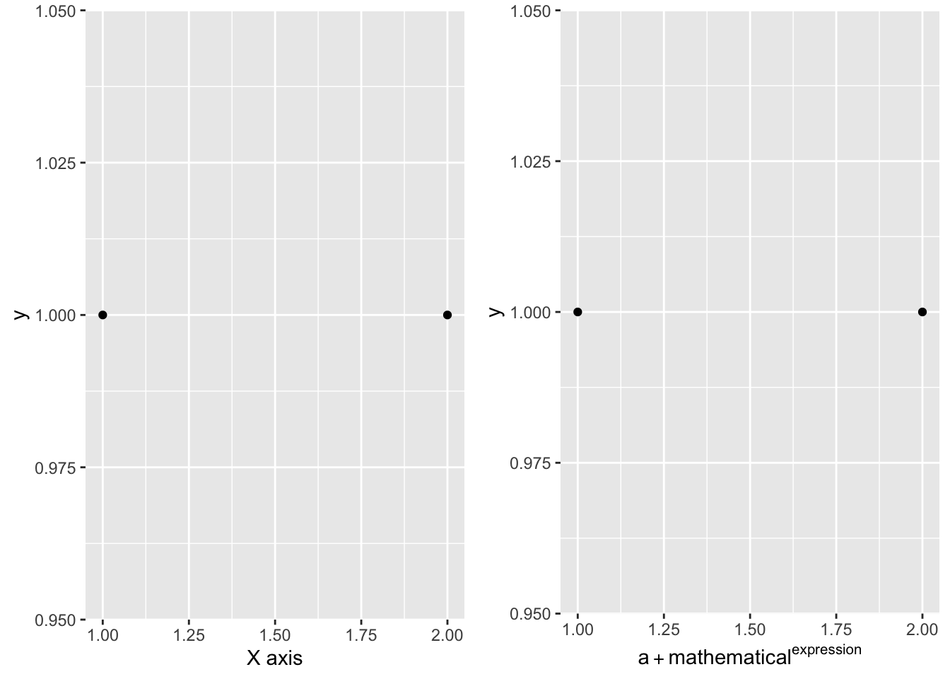
#labeling a scale
p <- ggplot(df, aes(x, y)) +
  geom_point(aes(colour = z))
p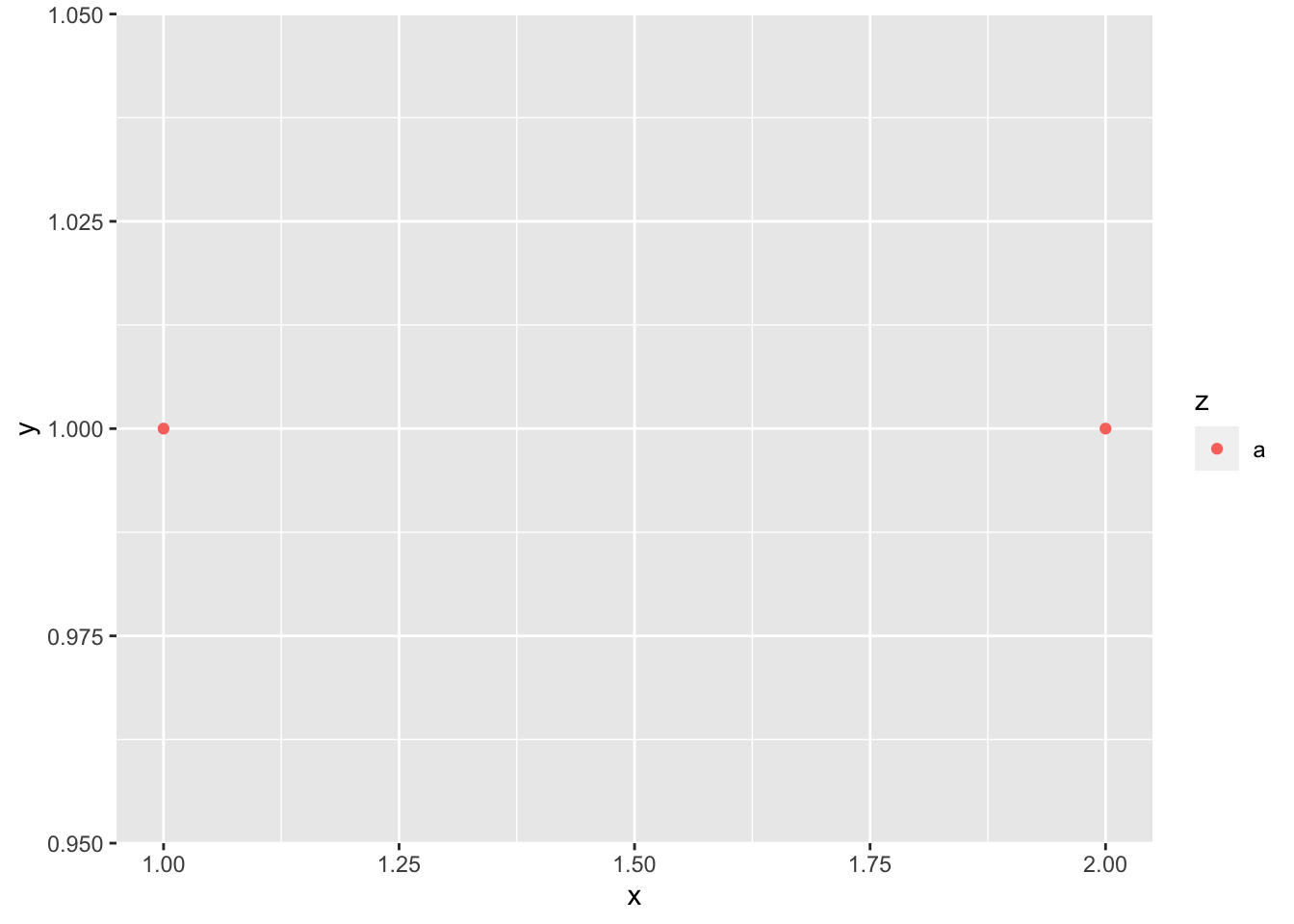
p1 = p + xlab("X axis") + ylab("Y axis")
p1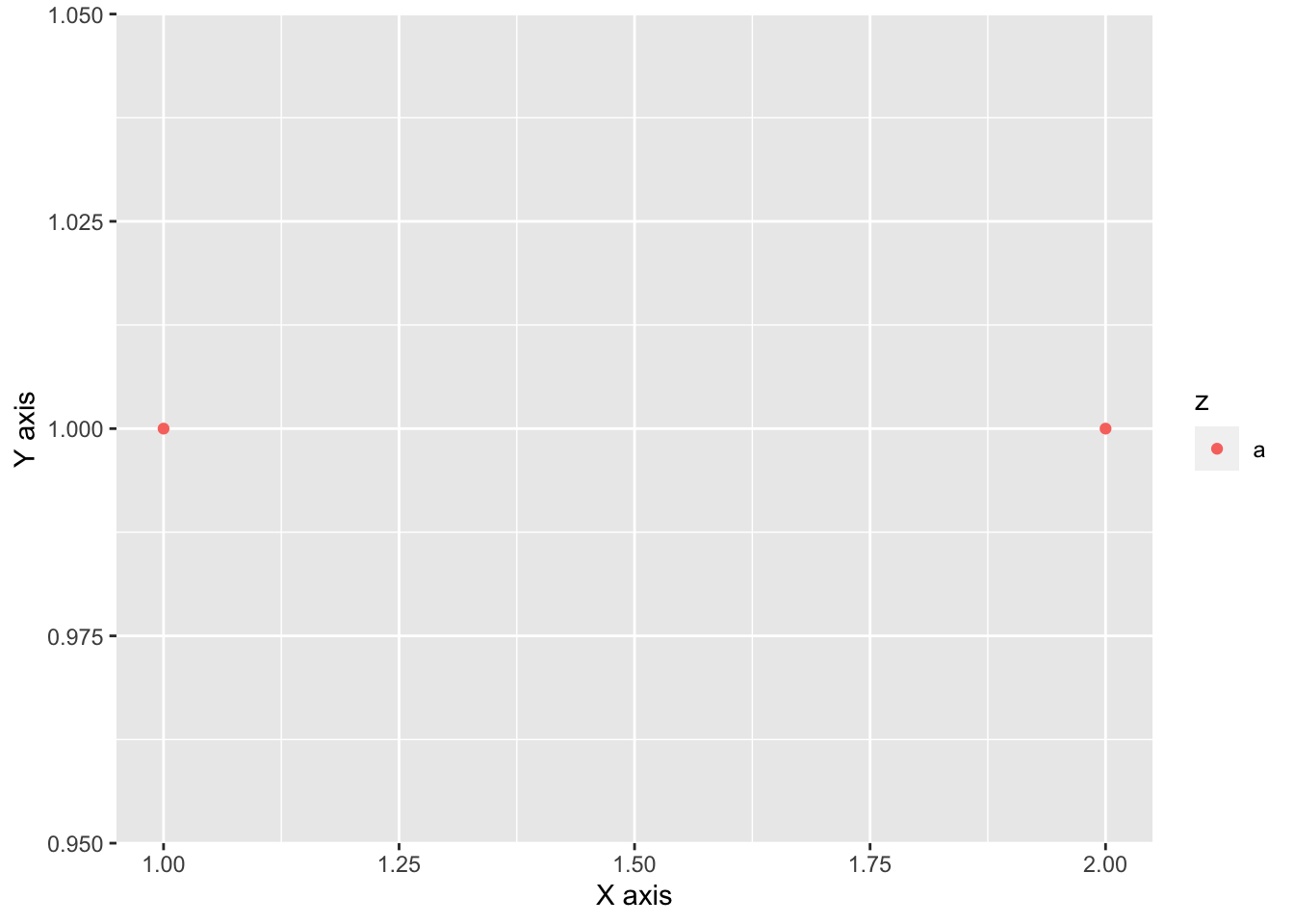
p2 = p + labs(x = "X axis", y = "Y axis",
              colour = "Colour\nlegend")
p2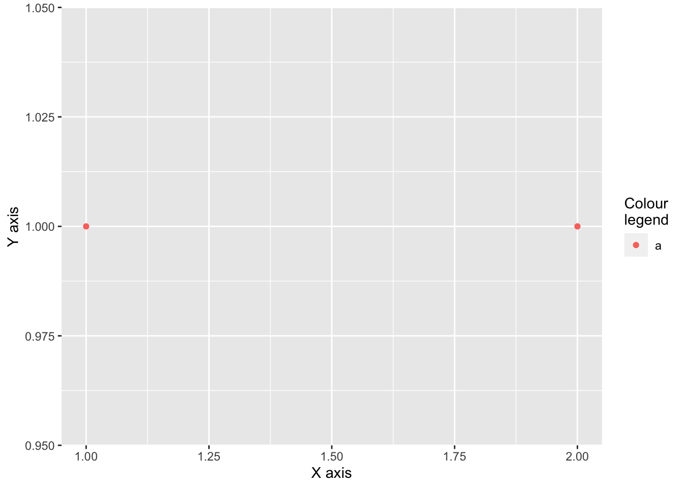
grid.arrange(p1,p2, ncol=2)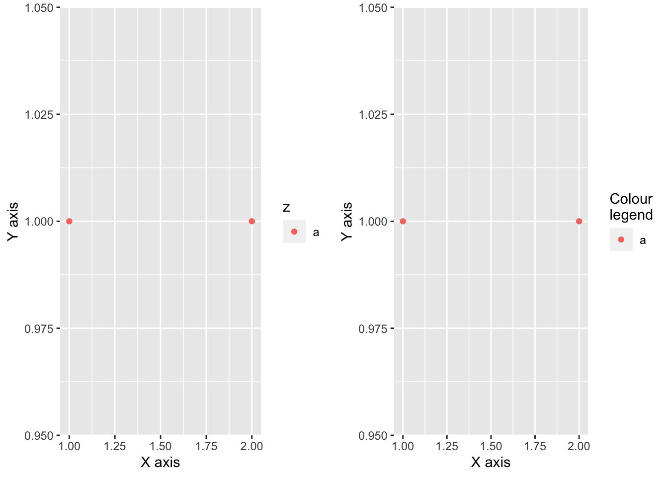
#\n is a shortcode for letting R know that you wish to have a new line.

#breaks and labels
df <- data.frame(x = c(1, 3, 5) * 1000, y = 1)
df
## x y
## 1 1000 1
## 2 3000 1
## 3 5000 1axs <- ggplot(df, aes(x, y)) +
geom_point() +
labs(x = NULL, y = NULL)
axs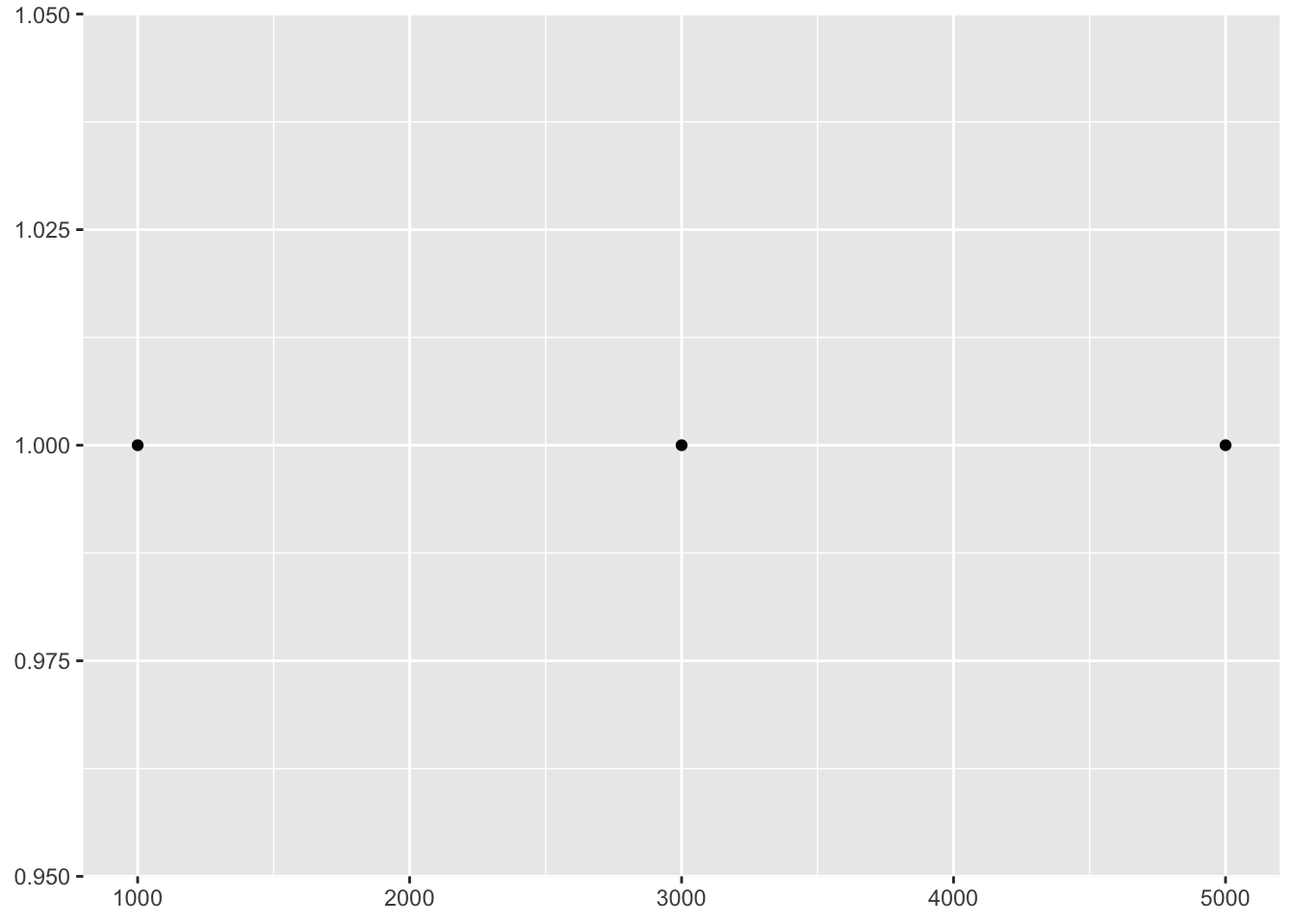
axs + scale_x_continuous(breaks = c(2000, 4000))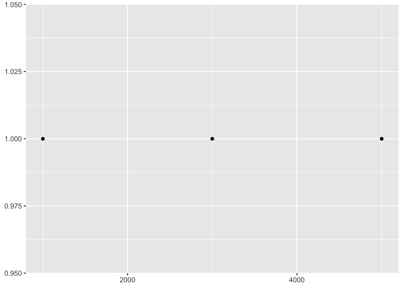
axs + scale_x_continuous(breaks = c(2000, 4000), labels = c("2k", "4k"))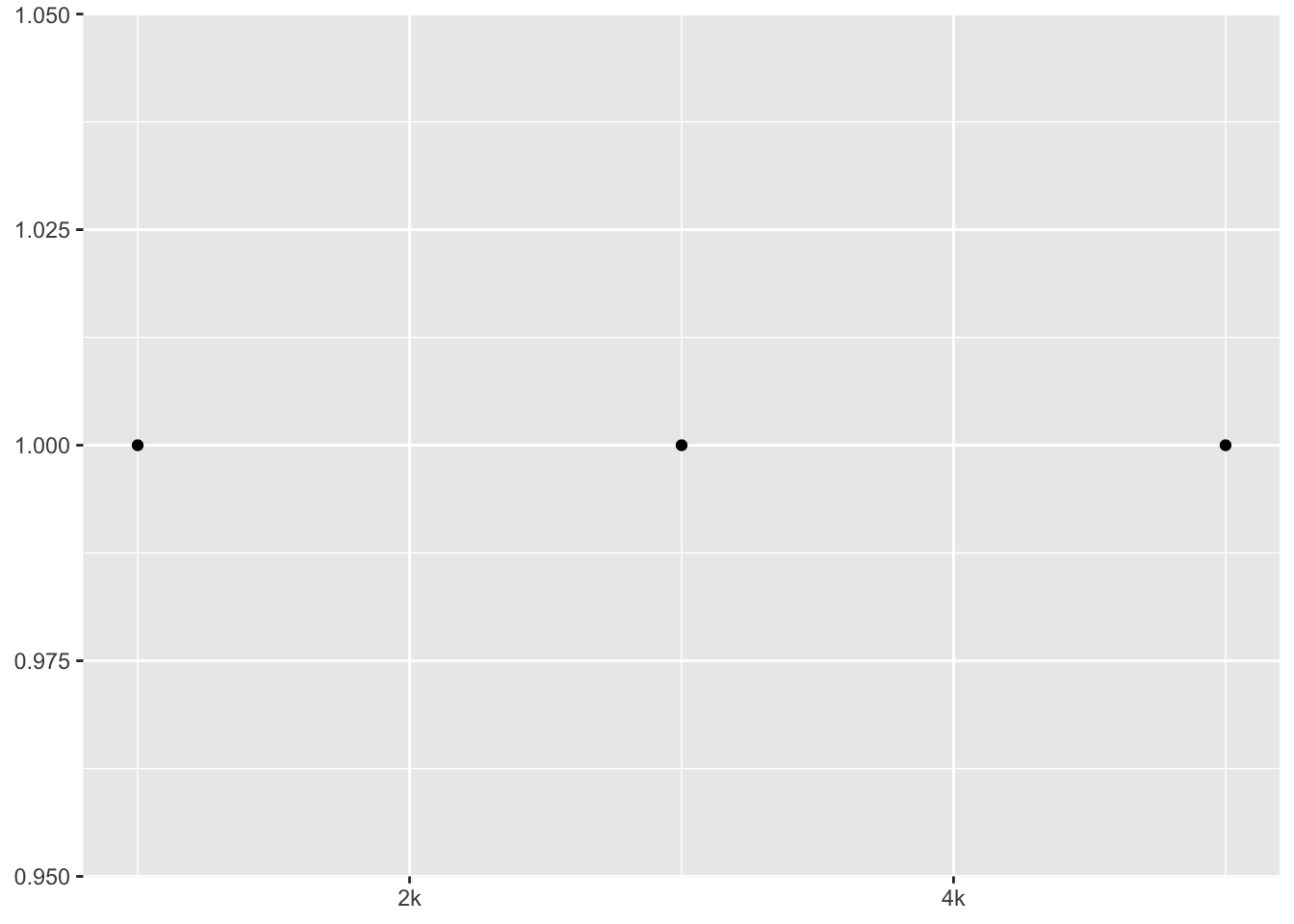
leg <- ggplot(df, aes(y, x, fill = x)) +
  geom_tile() +
  labs(x = NULL, y = NULL)
leg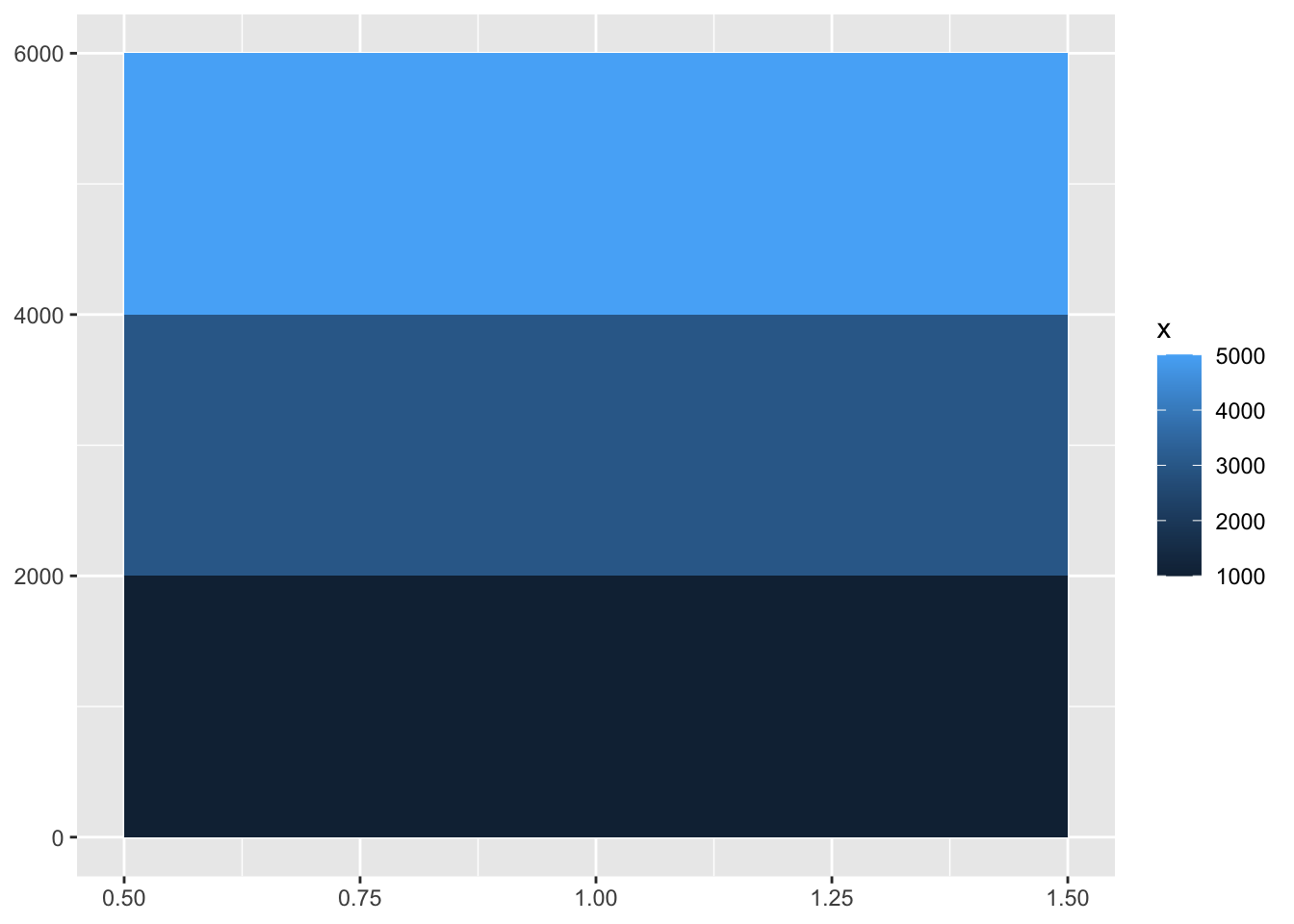
leg + scale_fill_continuous(breaks = c(2000, 4000))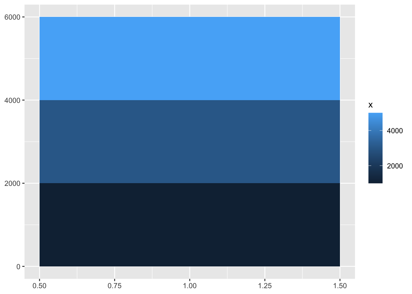
leg + scale_fill_continuous(breaks = c(2000, 4000), labels = c("2k", "4k"))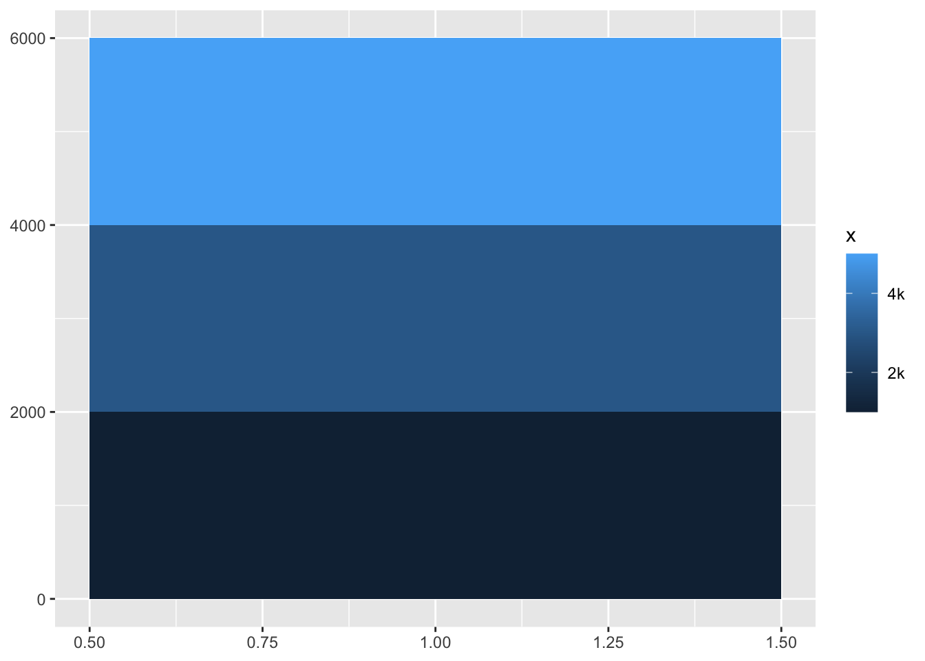
df2 <- data.frame(x = 1:3, y = c("a", "b", "c"))
df2
## x y
## 1 1 a
## 2 2 b
## 3 3 cggplot(df2, aes(x, y)) +
geom_point()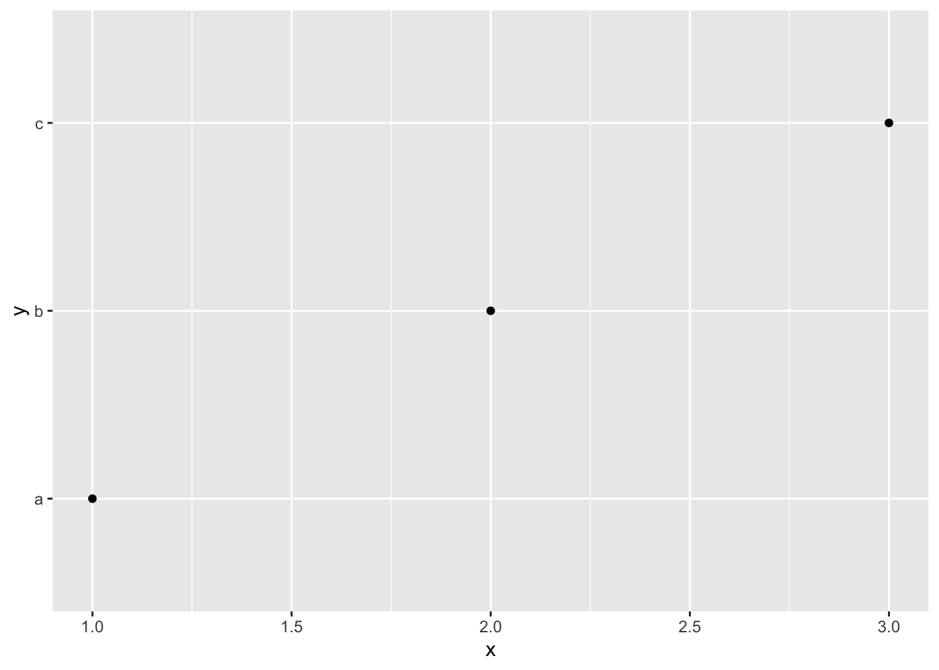
ggplot(df2, aes(x, y)) +
geom_point() +
scale_y_discrete(labels = c(a = "apple",
b = "banana", c = "carrot"))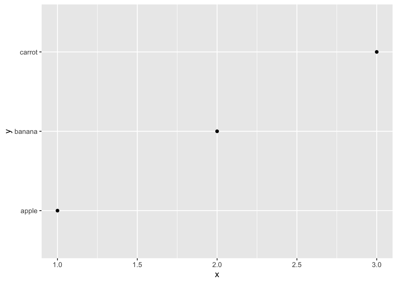
#########
#legends#
#########

norm <- data.frame(x = rnorm(1000), y = rnorm(1000))
mean(norm$x); mean(norm$y)
## [1] 0.04762906## [1] -0.05774357sd(norm$x); sd(norm$y)## [1] 0.9744101## [1] 0.983496norm$z <- cut(norm$x, 3, labels = c("a", "b", "c"))
sample_n(norm, 10)## x y z
## 1 -0.60623839 0.9007371 b
## 2 0.09938313 -0.5054266 b
## 3 -0.54075971 1.5324225 b
## 4 0.24860513 -1.5381656 b
## 5 -1.22423755 -0.8305189 b
## 6 -0.32323822 -0.2172429 b
## 7 0.19095299 -1.7205673 b
## 8 0.91717762 -1.0818583 c
## 9 -1.69316984 -0.6508852 a
## 10 -0.39645303 -0.8899890 bggplot(norm, aes(x, y)) +
geom_point(aes(colour = z), alpha = 0.1)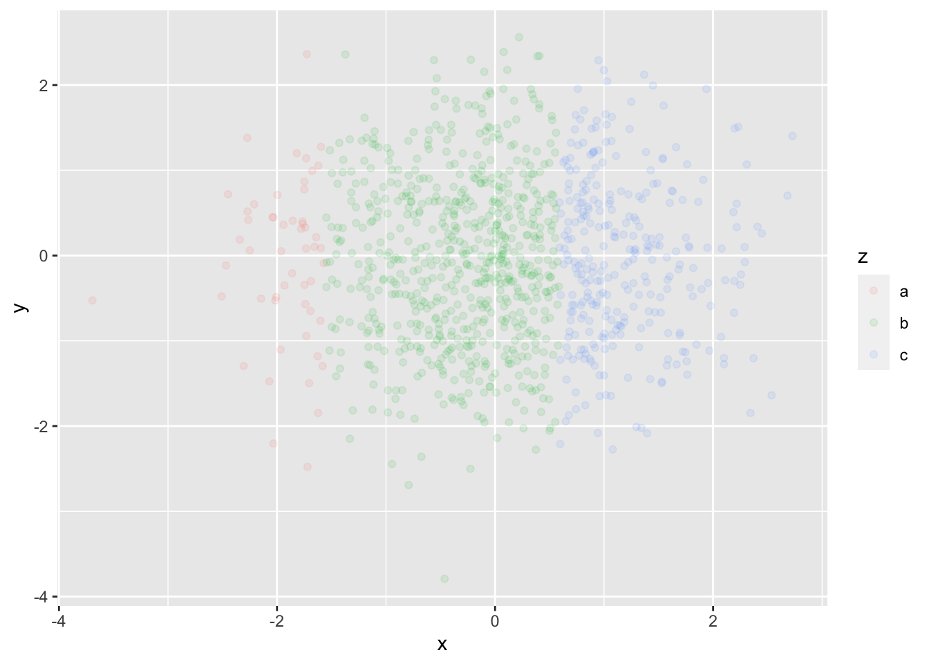
ggplot(norm, aes(x, y)) +
geom_point(aes(colour = z), alpha = 0.1) +
guides(colour = guide_legend(override.aes = list(alpha = 1)))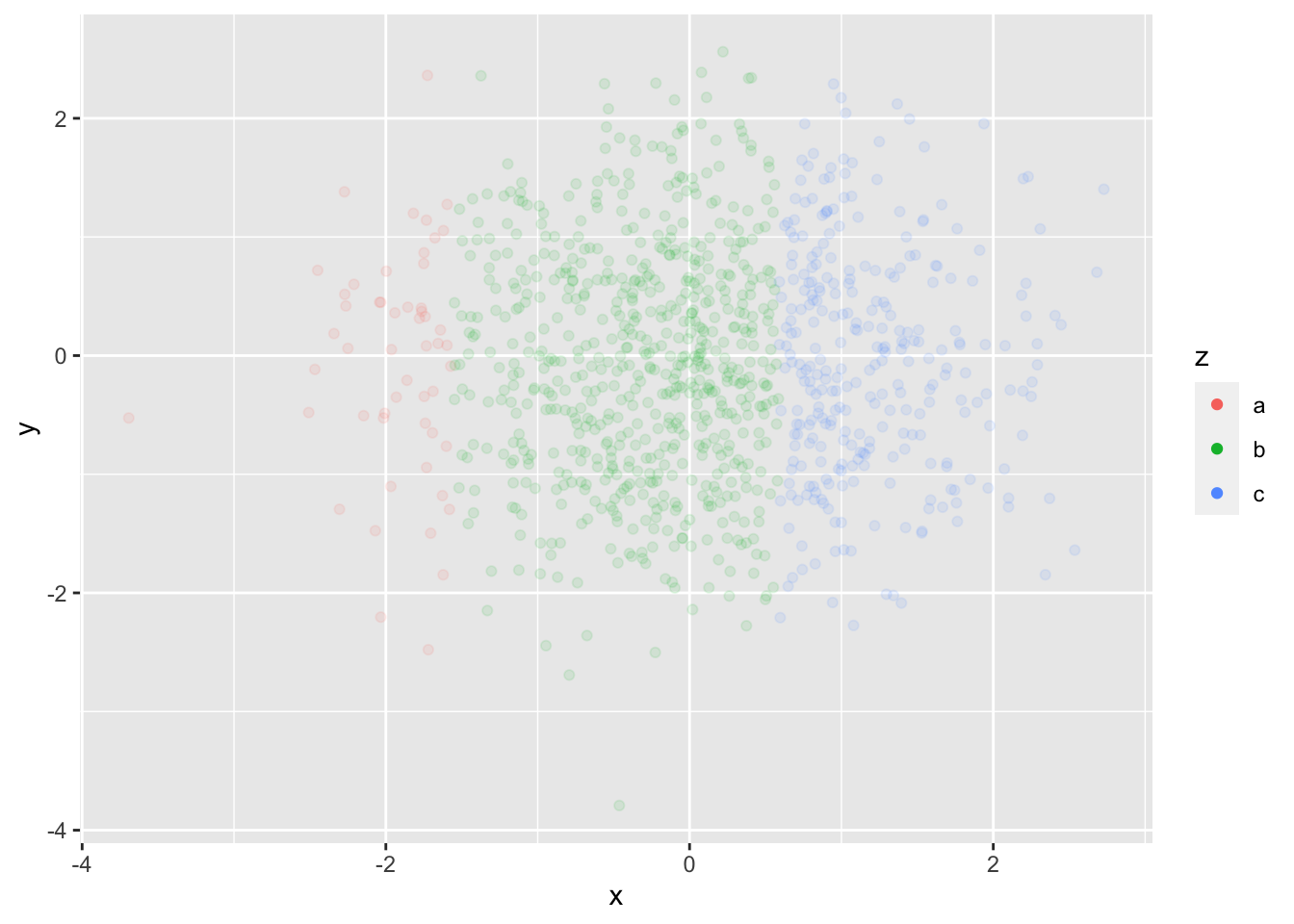
#legend layouts
df <- data.frame(x = 1:3, y = 1:3, z = c("a", "b", "c"))
base <- ggplot(df, aes(x, y)) +
  geom_point(aes(colour = z), size = 3) +
  xlab(NULL) +
  ylab(NULL)
base
base + theme(legend.position = "right") # the default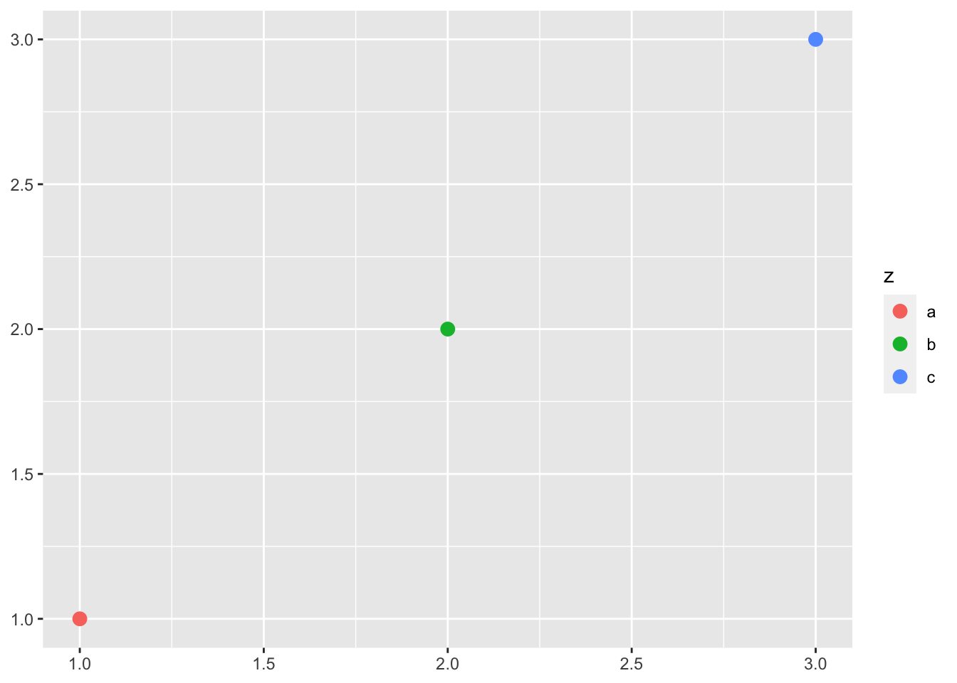
base + theme(legend.position = "bottom")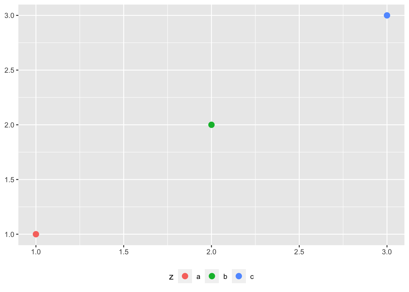
base + theme(legend.position = "none")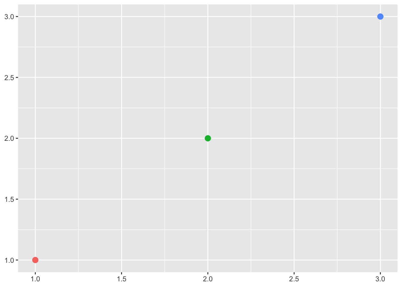
####################################
#extended example and using ggplot2#
####################################
require(ggplot2)
require(ggrepel)
dat <- read.csv("https://drive.google.com/uc?export=download&id=0B8CsRLdwqzbzUDJLa1owSVduLTA")
sample_n(dat,6)
## X Country HDI.Rank HDI CPI Region
## 1 125 Philippines 112 0.644 2.6 Asia Pacific
## 2 58 Gambia 168 0.420 3.5 SSA
## 3 98 Malaysia 61 0.761 4.3 Asia Pacific
## 4 139 Sierra Leone 180 0.336 2.5 SSA
## 5 123 Paraguay 107 0.665 2.2 Americas
## 6 103 Mauritius 77 0.728 5.1 SSA# Calls data then the asthetics are x,y and how coloring works
pc1 <- ggplot(dat, aes(x=CPI, y=HDI, color=Region))
#geom_point() is how we choose points to be plotted
pc1 + geom_point()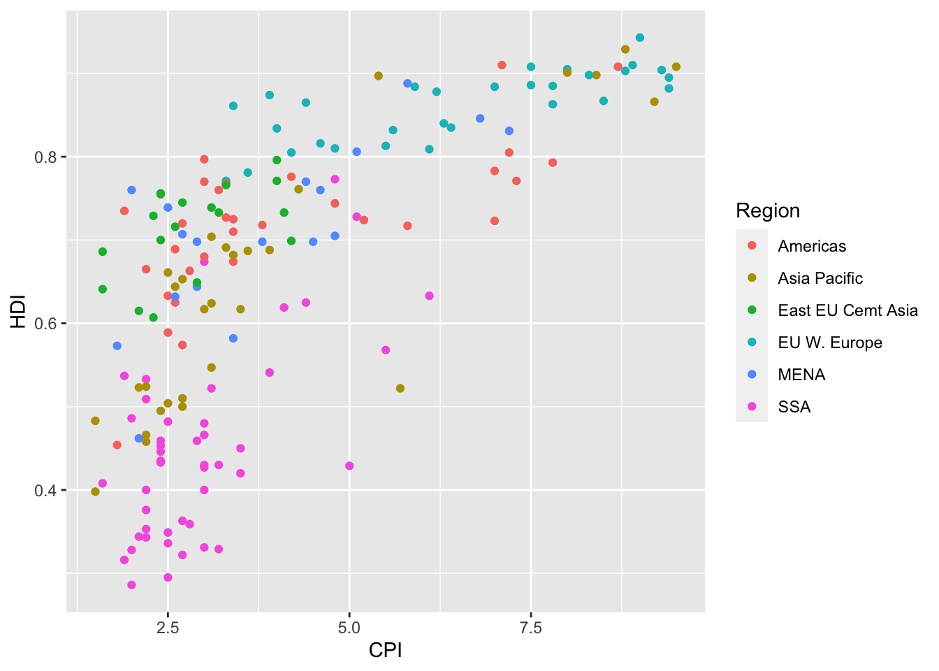
(pc2 <- pc1 +
    geom_smooth(aes(group = 1),
                method = "lm",
                formula = y ~ log(x),
                se = FALSE,
                color = "red")) +
  geom_point()
#change point shape
## A look at all 25 symbols
## A look at all 25 symbols
df2 <- data.frame(x = 1:5 , y = 1:25, z = 1:25)
s <- ggplot(df2, aes(x = x, y = y)) +
  geom_point(aes(shape = z), size = 4) +
  scale_shape_identity() +
  geom_point(aes(shape = z), size = 4, colour = "Red") +
  scale_shape_identity() +
  geom_point(aes(shape = z), size = 4, colour = "Red", fill = "Black") +
  scale_shape_identity()
## Scale for 'shape' is already present. Adding another scale for 'shape', which will replace the existing scale.## Scale for 'shape' is already present. Adding another scale for 'shape', which will replace the existing scale.s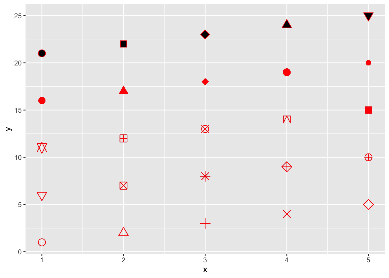
pc2 + geom_point(shape=1, size=4)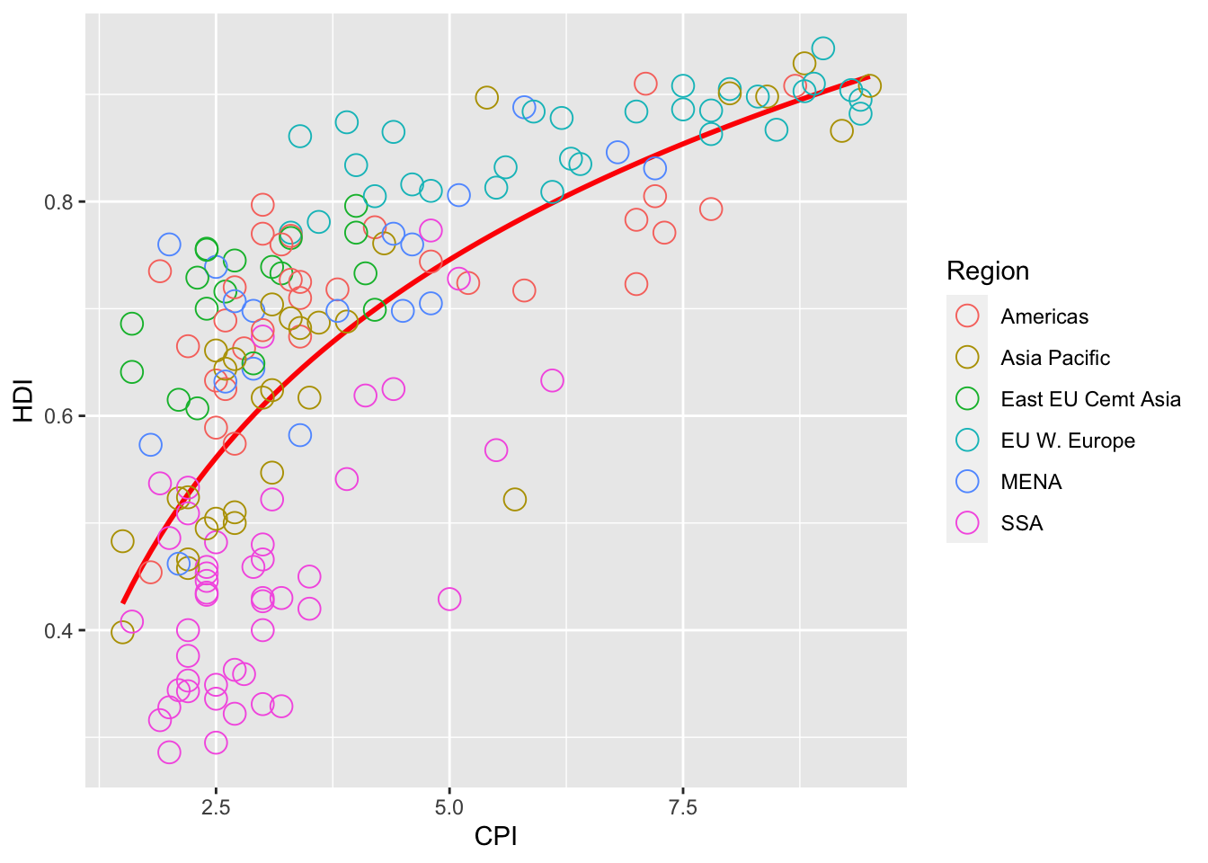
(pc3 <- pc2 +
    geom_point(size = 4.2, shape = 1) +
    geom_point(size = 4.3, shape = 1) +
    geom_point(size = 4.1, shape = 1) +
    geom_point(size = 4, shape = 1) +
    geom_point(size = 3.9, shape = 1) +
    geom_point(size = 3.8, shape = 1)+
    geom_point(size = 3.5, shape = 1))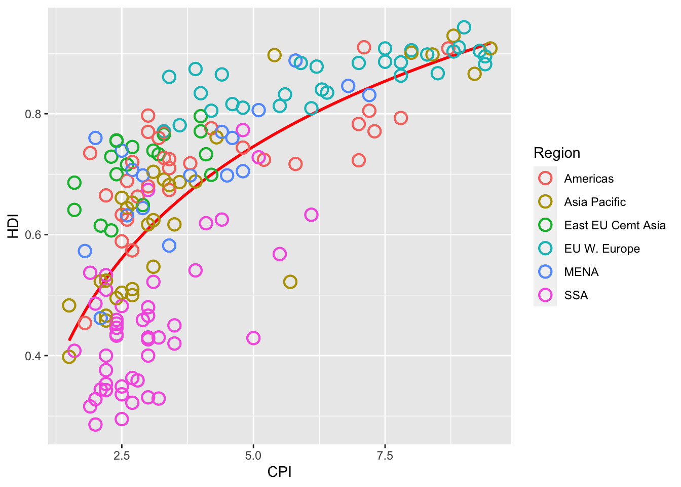
(pc3 <- pc2 +
  geom_point(size = 3, shape = 1) +
  geom_point(size = 4, shape = 1))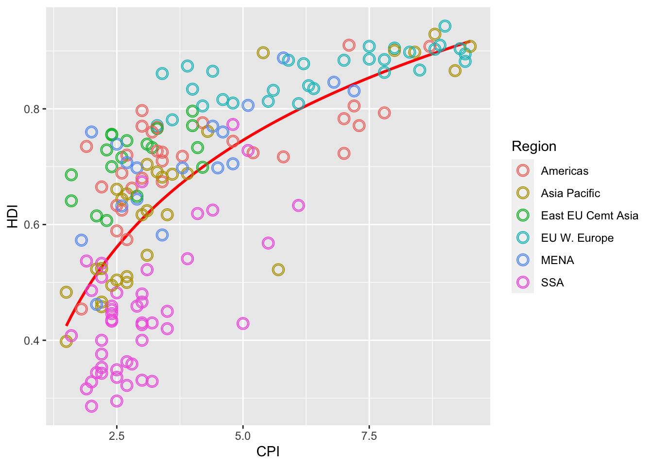
pointsToLabel <- c("Russia", "Venezuela", "Iraq", "Myanmar", "Sudan",
                   "Afghanistan", "Congo", "Greece", "Argentina", "Brazil",
                   "India", "Italy", "China", "South Africa", "Spane",
                   "Botswana", "Cape Verde", "Bhutan", "Rwanda", "France",
                   "United States", "Germany", "Britain", "Barbados", "Norway", "Japan",
                   "New Zealand", "Singapore")
pc3 +
  geom_text(aes(label = Country),
            color = "gray20",
            data = subset(dat, Country %in% pointsToLabel))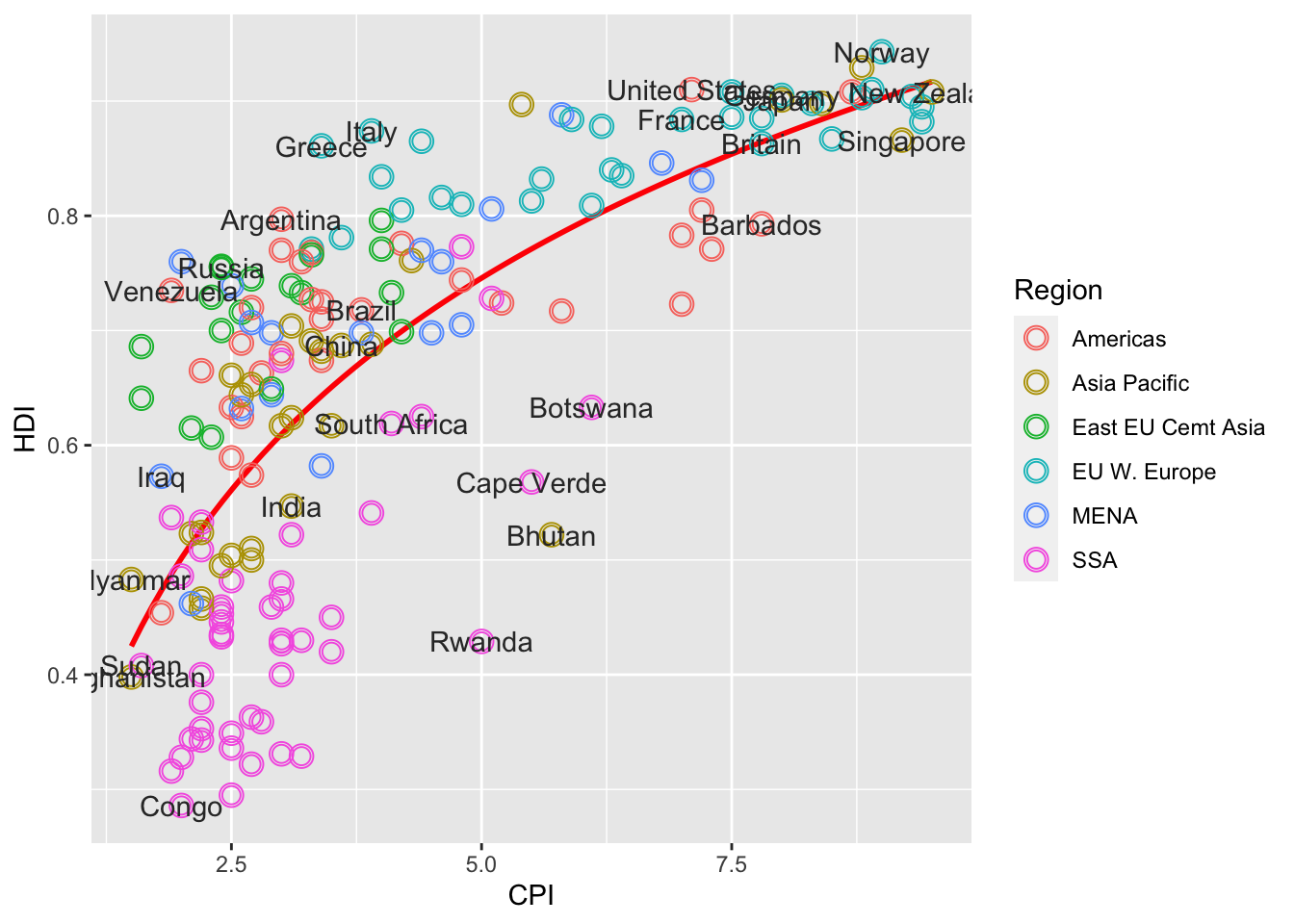
library("ggrepel")
(pc4 <-pc3 +
    geom_text_repel(aes(label = Country),
                    color = "gray20",
                    data = subset(dat, Country %in% pointsToLabel),
                    force = 10))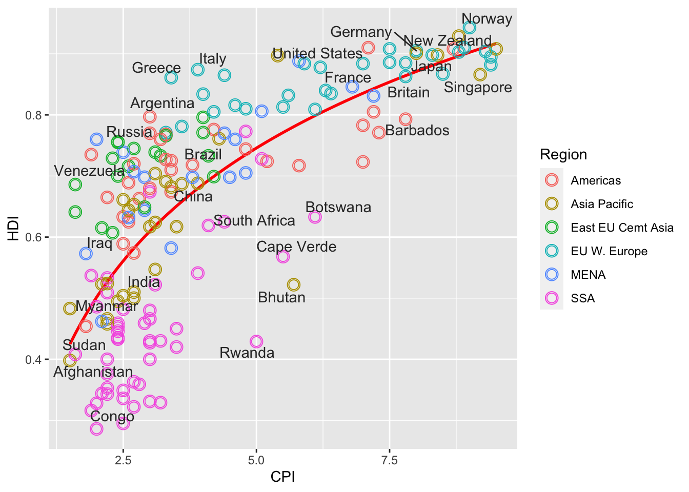
#change region labels and order
dat$Region <- factor(dat$Region,
                     levels = c("EU W. Europe",
                                "Americas",
                                "Asia Pacific",
                                "East EU Cemt Asia",
                                "MENA",
                                "SSA"),
                     labels = c("OECD",
                                "Americas",
                                "Asia &\nOceania",
                                "Central &\nEastern Europe",
                                "Middle East &\nNorth Africa",
                                "Sub-Saharan\nAfrica"))
head(pc4$data)
## X Country HDI.Rank HDI CPI Region
## 1 1 Afghanistan 172 0.398 1.5 Asia Pacific
## 2 2 Albania 70 0.739 3.1 East EU Cemt Asia
## 3 3 Algeria 96 0.698 2.9 MENA
## 4 4 Angola 148 0.486 2.0 SSA
## 5 5 Argentina 45 0.797 3.0 Americas
## 6 6 Armenia 86 0.716 2.6 East EU Cemt Asiapc4$data <- dat
pc4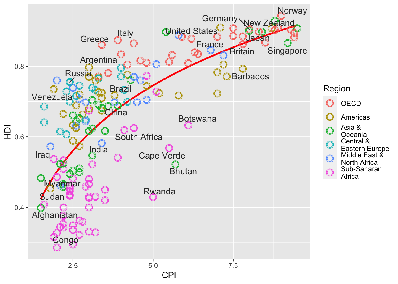
#add title and format axes
library(grid)
pc5 <- pc4 +
  scale_x_continuous(name = "Corruption Perceptions Index, 2011 (10=least corrupt)",
                     limits = c(.9, 10.5),
                     breaks = 1:10) +
  scale_y_continuous(name = "Human Development Index, 2011 (1=Best)",
                     limits = c(0.2, 1.0),
                     breaks = seq(0.2, 1.0, by = 0.1)) +
  scale_color_manual(name = "",
                     values = c("#24576D",
                                "#099DD7",
                                "#28AADC",
                                "#248E84",
                                "#F2583F",
                                "#96503F")) +
  ggtitle("Corruption and Human development")
pc5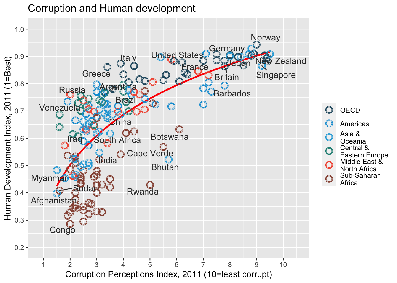
#final changes to the output
pc6 <- pc5 +
  theme_minimal() + # start with a minimal theme and add what we need
  theme(text = element_text(color = "gray20"),
        legend.position = c("top"), # position the legend in the upper left
        legend.direction = "horizontal",
        legend.justification = 0.1, # anchor point for legend.position.
        legend.text = element_text(size = 11, color = "gray10"),
        axis.text = element_text(face = "italic"),
        axis.title.x = element_text(vjust=-10), # move title away from axis
        axis.title.y = element_text(vjust = 2), # move away for axis
        axis.ticks.y = element_blank(), # element_blank() is how we remove elements
        axis.line = element_line(color = "gray40", size = 0.5),
        axis.line.y = element_blank(),
        panel.grid.major = element_line(color = "gray50", size = 0.5),
        panel.grid.major.x = element_blank()
  )
pc6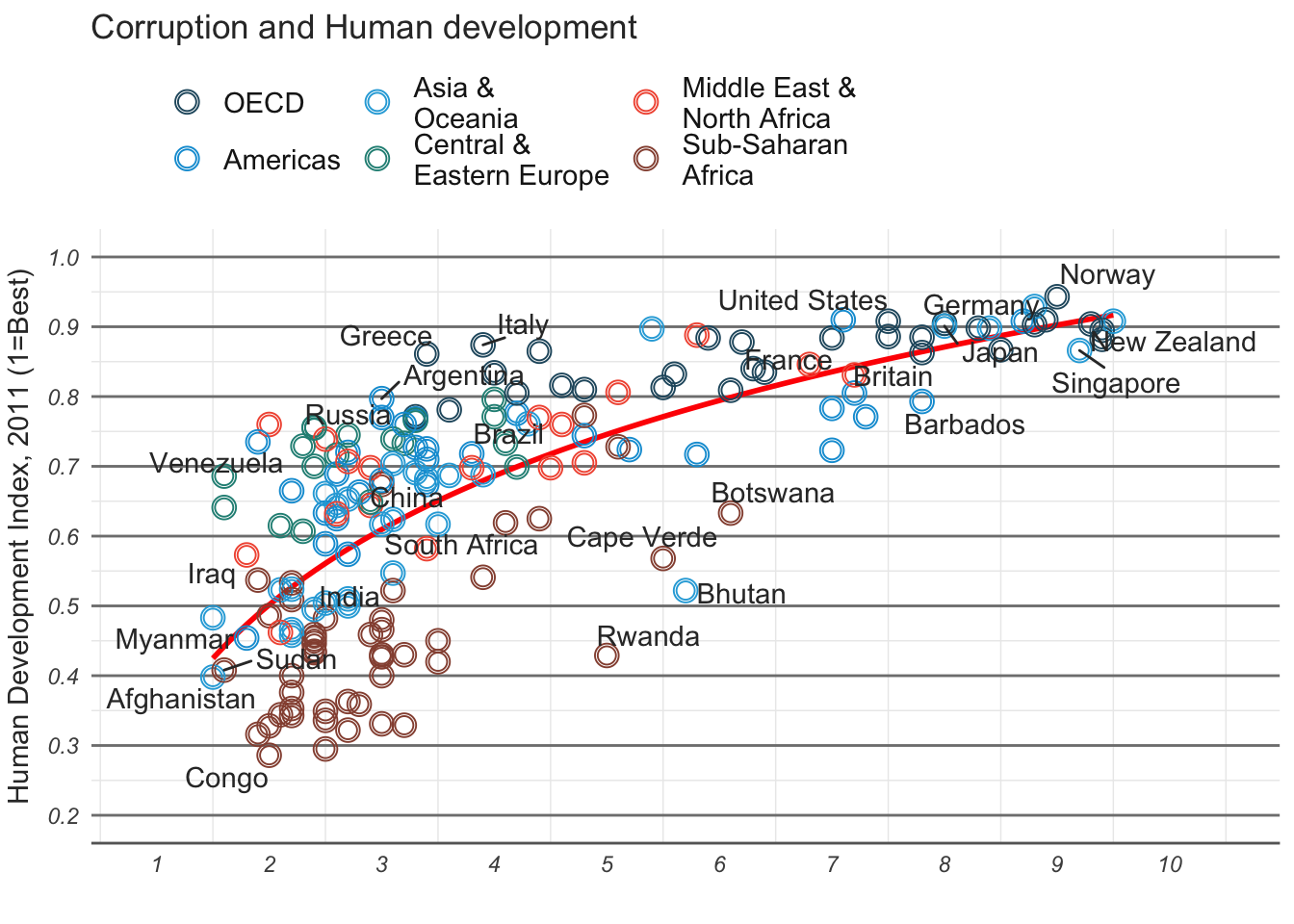
#add R^2
mR2 <- summary(lm(HDI ~ log(CPI), data = dat))$r.squared

library(grid)
#png(file = "images/econScatter10.png", width = 800, height = 600)
pc6
grid.text("Sources: Transparency International; UN Human Development Report",
          x = .01, y = .01,
          just = "left",
          draw = TRUE,  gp=gpar(fontsize=7, col="grey"))
grid.segments(x0 = 0.81, x1 = 0.825,
              y0 = 0.90, y1 = 0.90,
              gp = gpar(col = "red"),
              draw = TRUE)
grid.text(paste0("R^2 = ",
                 as.integer(mR2*100),
                 "%"),
          x = 0.835, y = 0.90,
          gp = gpar(col = "gray20"),
          draw = TRUE,
          just = "left")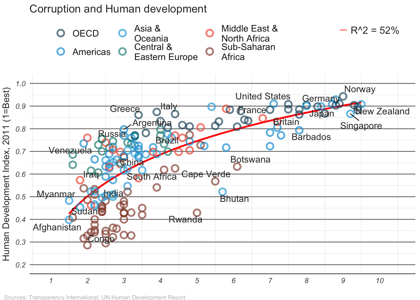
#dev.off()