Chapter 5 Exploratory Data Analysis
Topics covered:
- Need to know the use of count(cut_width(continuous, interval)) for countinous var.
- geom_freqpoly to overlay multiple histograms, coord_cartesian to zoom in
- use of ..density.. in aes()
- geom_tile()
- reorder(x, y, FUN), count(), mutate(), %%, %/%, cut_number()
- use geom_bin2d() and hexbin() to bin into two dimensions
5.1 visualizing distributions
#visualizing distributions
ggplot(data = diamonds)+
  geom_bar(mapping = aes(x=cut))
diamonds %>%
  count(cut)
## # A tibble: 5 x 2
## cut n
## * <ord> <int>
## 1 Fair 1610
## 2 Good 4906
## 3 Very Good 12082
## 4 Premium 13791
## 5 Ideal 21551ggplot(data=diamonds)+
geom_histogram(mapping = aes(x=carat), binwidth = 0.5)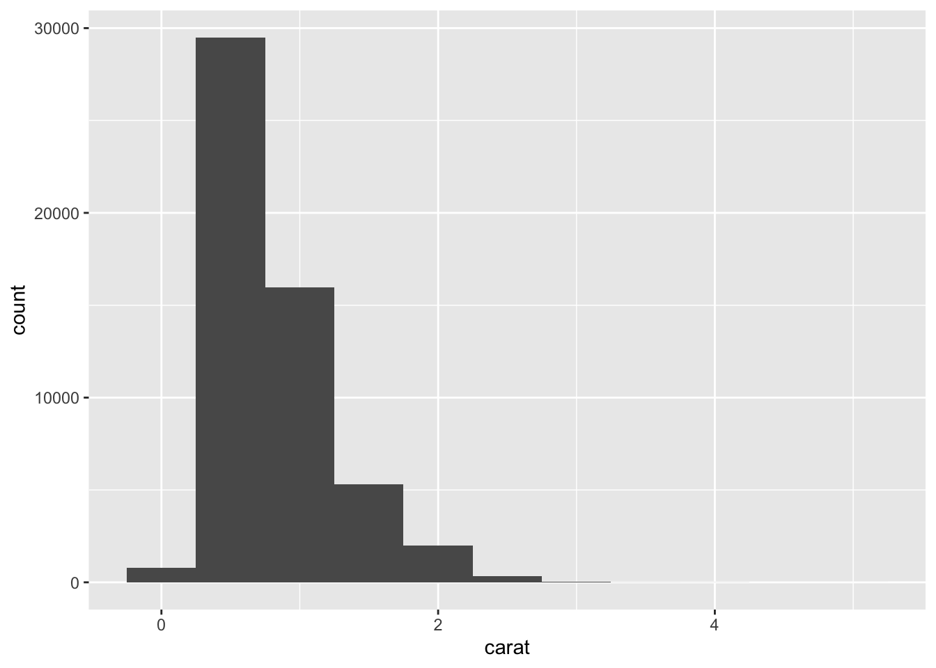
diamonds %>%
  count(cut_width(carat, 0.5))
## # A tibble: 11 x 2
## `cut_width(carat, 0.5)` n
## * <fct> <int>
## 1 [-0.25,0.25] 785
## 2 (0.25,0.75] 29498
## 3 (0.75,1.25] 15977
## 4 (1.25,1.75] 5313
## 5 (1.75,2.25] 2002
## 6 (2.25,2.75] 322
## 7 (2.75,3.25] 32
## 8 (3.25,3.75] 5
## 9 (3.75,4.25] 4
## 10 (4.25,4.75] 1
## 11 (4.75,5.25] 1#let's zoom in
smaller <- diamonds %>%
filter(carat<3)
ggplot(data = smaller, mapping = aes(x=carat))+
geom_histogram(binwidth = .1)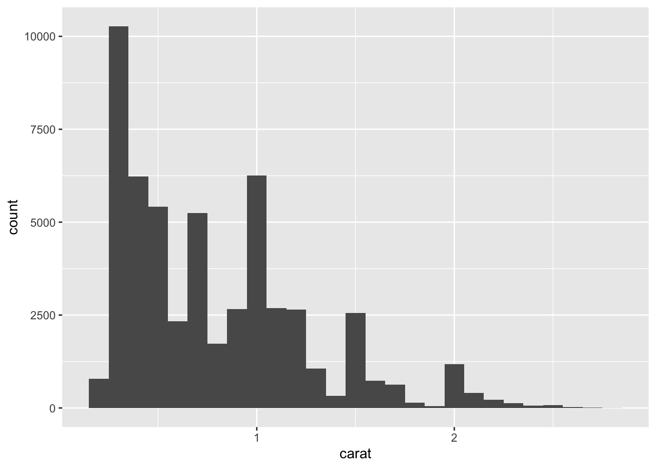
#overlay multiple histograms
ggplot(data = smaller, mapping = aes(x=carat, color=cut, fill=cut))+
  geom_freqpoly(binwidth=.1)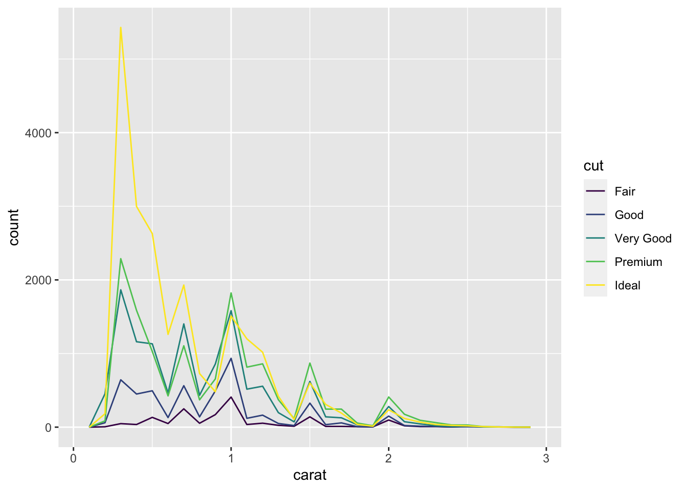
ggplot(data = smaller, mapping = aes(x=carat))+
  geom_histogram(binwidth = .01)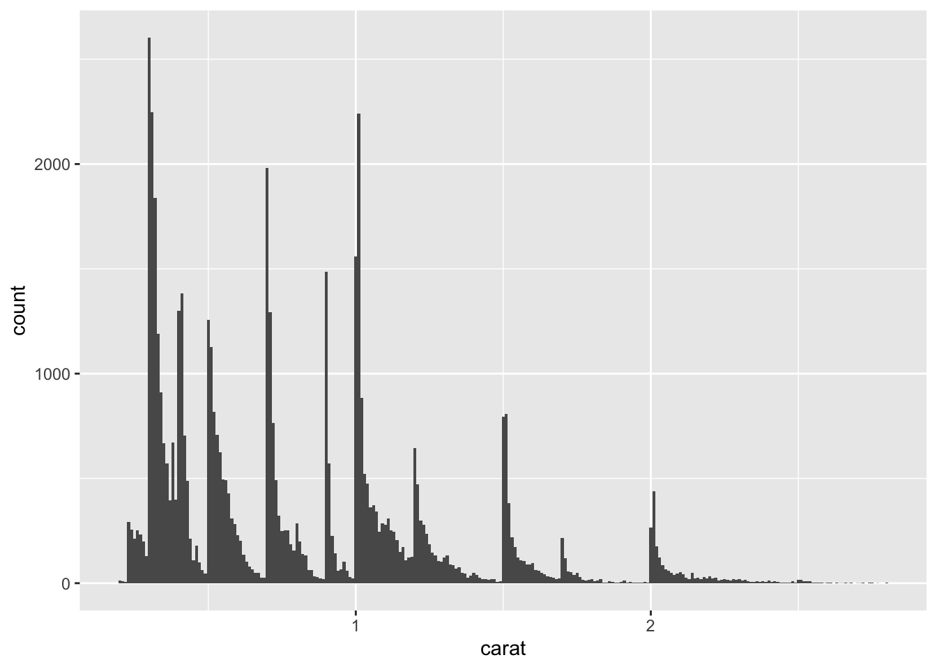
#check outliners
ggplot(diamonds)+
  geom_histogram(mapping = aes(x=y), binwidth = .5)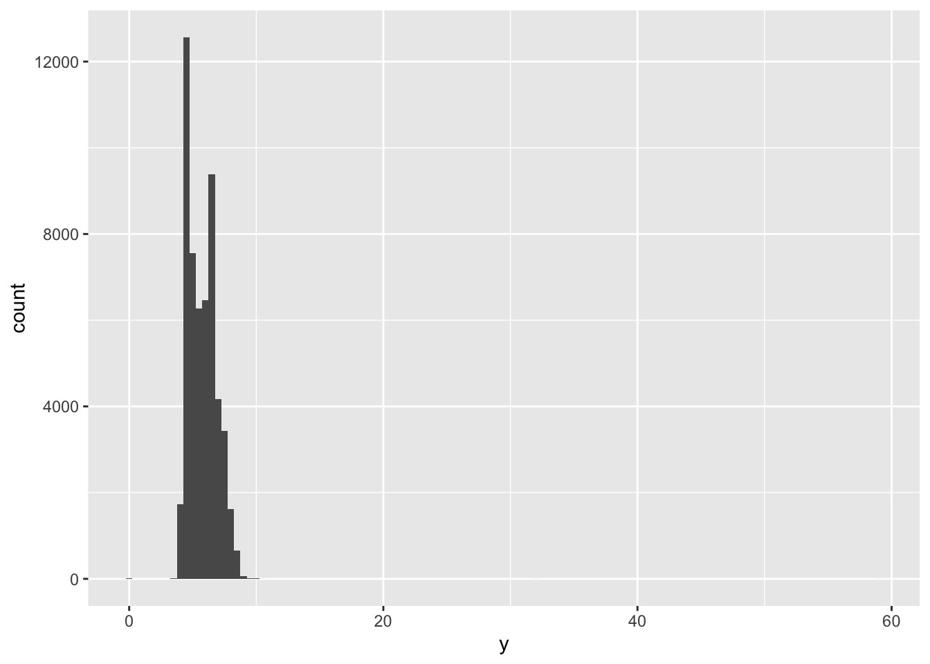
#zoom-in to small y values
ggplot(diamonds)+
  geom_histogram(mapping = aes(x=y), binwidth = .5)+
  coord_cartesian(ylim = c(0,50))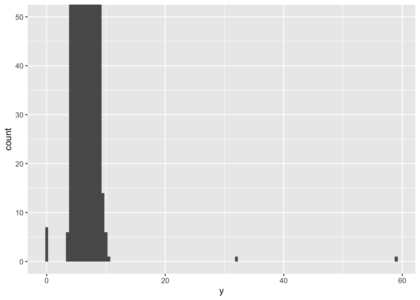
unusual <- diamonds %>%
  filter(y<3 | y>20) %>%
  arrange(y) #increasing by default

#missing values
#drop outliners
diamonds2 <- diamonds %>%
  filter(between(y, 3, 20))
#replacing unusual values with NA
diamonds2 <- diamonds %>%
  mutate(y=ifelse(y<3 | y>20, NA, y))
summary(diamonds2$y)
## Min. 1st Qu. Median Mean 3rd Qu. Max. NA's
## 3.680 4.720 5.710 5.734 6.540 10.540 9ggplot(data = diamonds2, mapping = aes(x=x, y=y))+
geom_point() #remove NA automatically## Warning: Removed 9 rows containing missing values (geom_point).
#can do this manually
ggplot(data = diamonds2, mapping = aes(x=x, y=y))+
  geom_point(na.rm = T)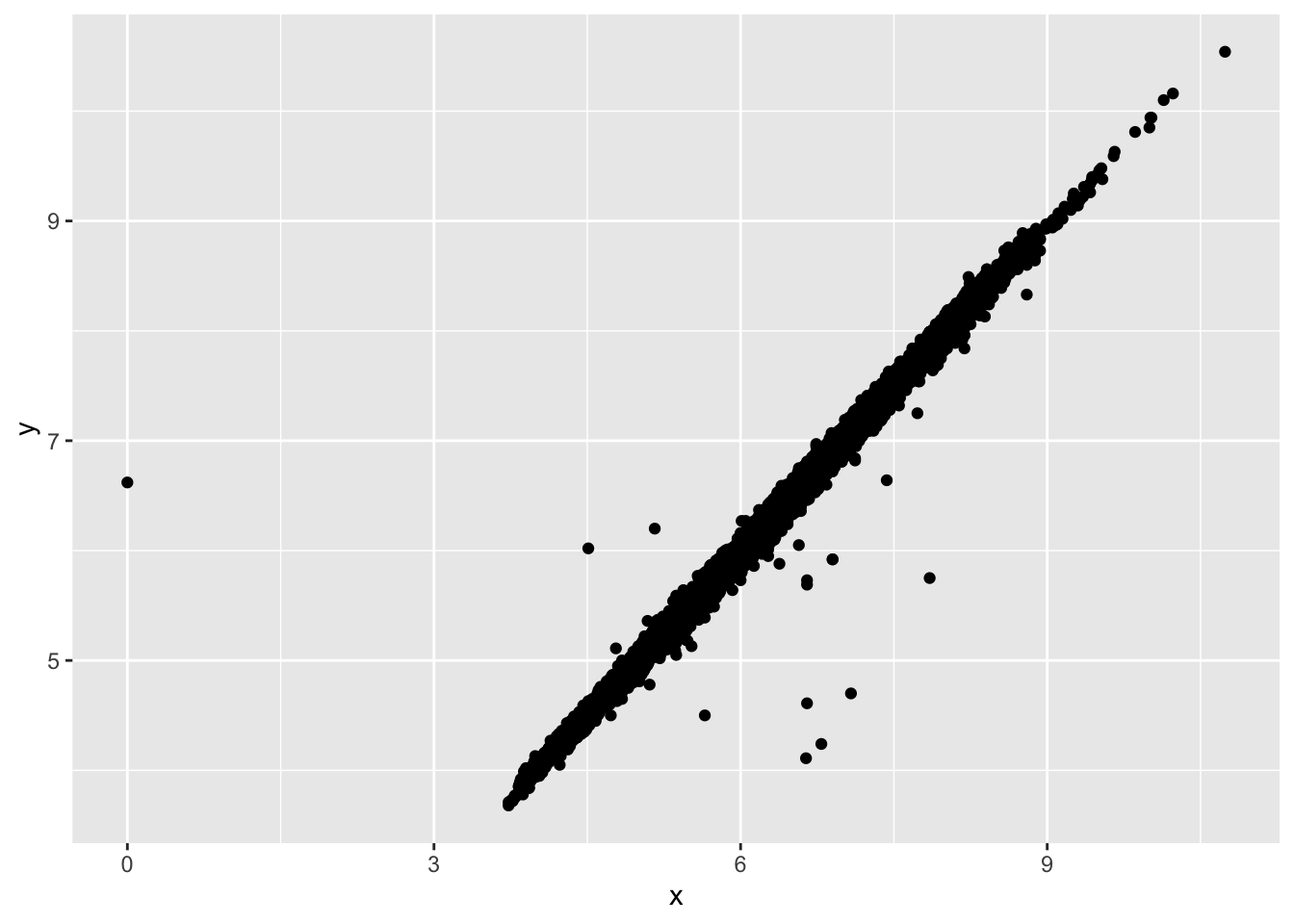
#compare
nycflights13::flights %>%
  mutate(
    cancelled = is.na(dep_time),
    sched_hour = sched_dep_time %/% 100,
    sched_min = sched_dep_time%%100,
    sched_dep_time = sched_hour + sched_min/60
  ) %>%
  ggplot(mapping = aes(sched_dep_time))+
  geom_freqpoly(mapping = aes(color=cancelled),
                binwidth=1/4)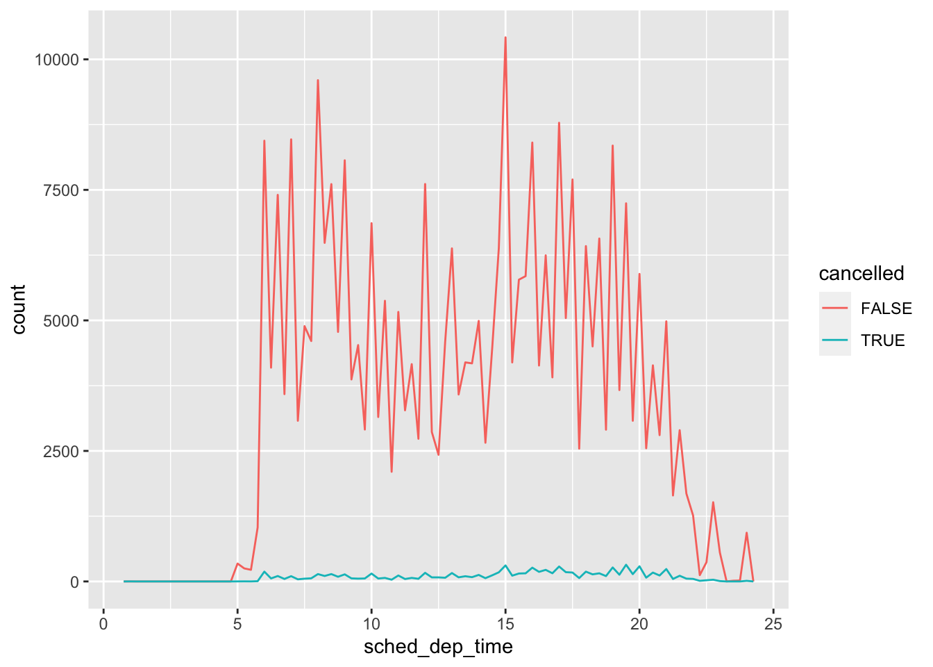
5.2 check covariation
#categorical and continuous
ggplot(data = diamonds, mapping = aes(x=price))+
  geom_freqpoly(mapping = aes(color=cut), binwidth=500)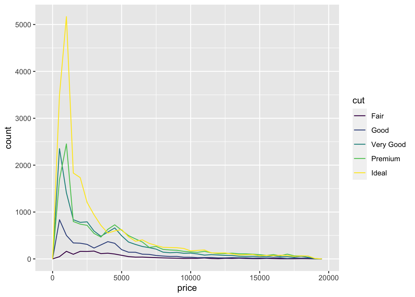
ggplot(diamonds)+
  geom_bar(aes(x=cut))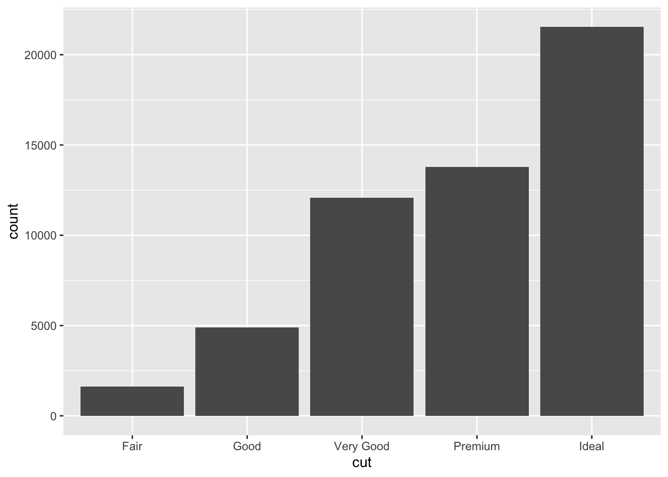
#display density
ggplot(data = diamonds, mapping = aes(x=price, y=..density..))+
  geom_freqpoly(mapping = aes(color=cut), binwidth=500)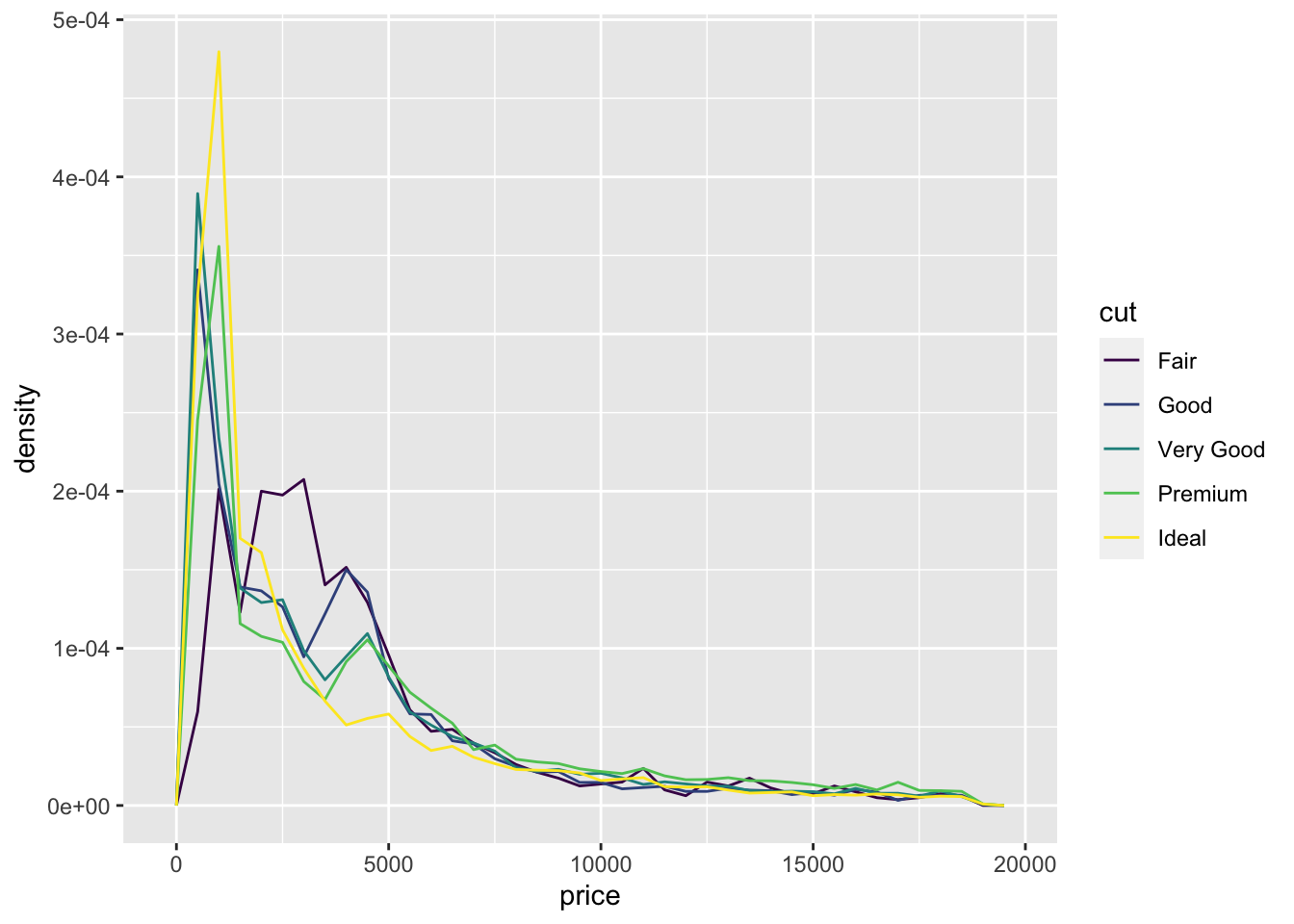
#it appears that fair diamonds have the highest average price

#boxplot
ggplot(data = diamonds, mapping = aes(x=cut, y=price))+
  geom_boxplot()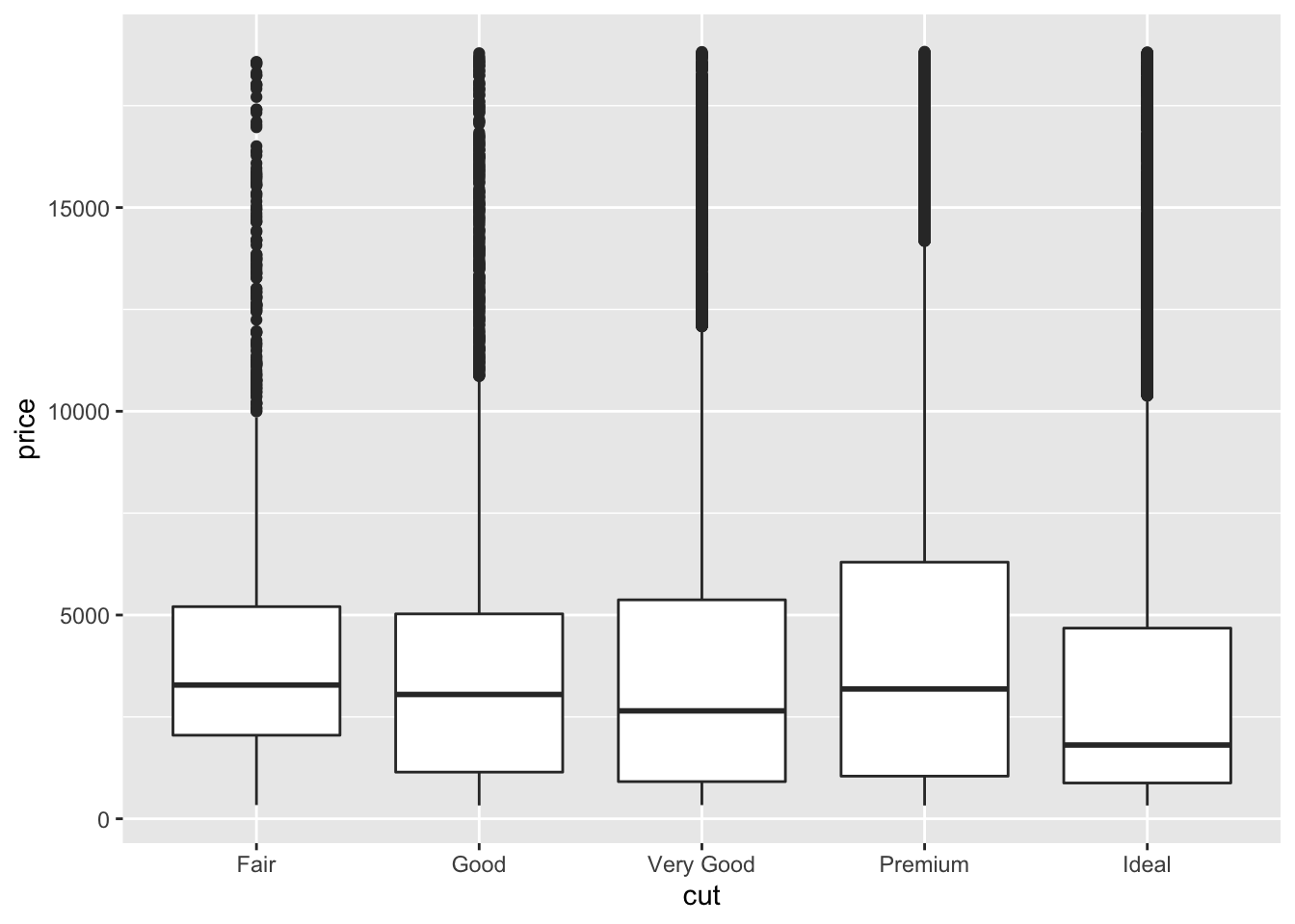
ggplot(data = mpg, mapping = aes(x=class, y=hwy))+
  geom_boxplot()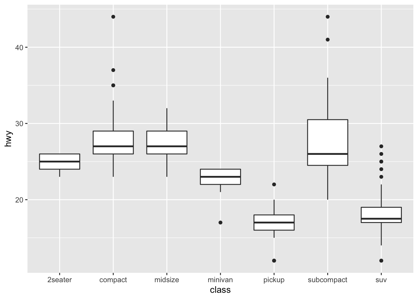
#reorder
ggplot(data = mpg, mapping = aes(x=reorder(class, hwy, FUN = median),
                                 y=hwy))+
  geom_boxplot()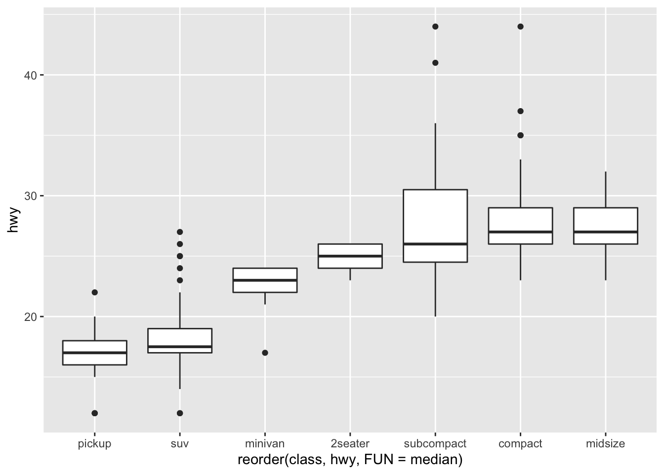
ggplot(data = mpg, mapping = aes(x=reorder(class, hwy, FUN = median),
                                 y=hwy))+
  geom_boxplot()+
  coord_flip()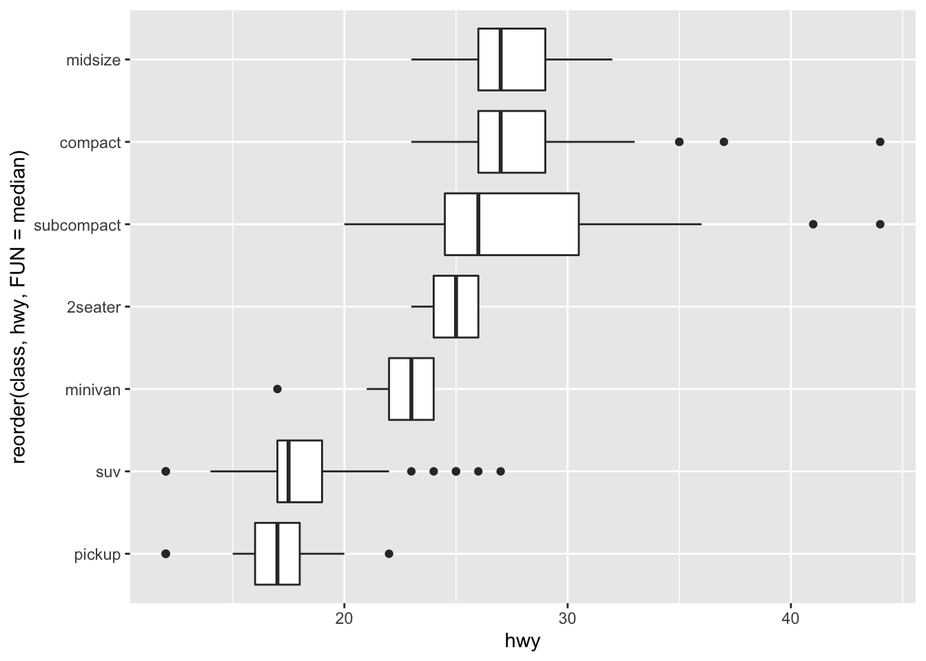
#two categorical variables
#the size of circle displays number of obs
diamonds
## # A tibble: 53,940 x 10
## carat cut color clarity depth table price x y z
## <dbl> <ord> <ord> <ord> <dbl> <dbl> <int> <dbl> <dbl> <dbl>
## 1 0.23 Ideal E SI2 61.5 55 326 3.95 3.98 2.43
## 2 0.21 Premium E SI1 59.8 61 326 3.89 3.84 2.31
## 3 0.23 Good E VS1 56.9 65 327 4.05 4.07 2.31
## 4 0.290 Premium I VS2 62.4 58 334 4.2 4.23 2.63
## 5 0.31 Good J SI2 63.3 58 335 4.34 4.35 2.75
## 6 0.24 Very Good J VVS2 62.8 57 336 3.94 3.96 2.48
## 7 0.24 Very Good I VVS1 62.3 57 336 3.95 3.98 2.47
## 8 0.26 Very Good H SI1 61.9 55 337 4.07 4.11 2.53
## 9 0.22 Fair E VS2 65.1 61 337 3.87 3.78 2.49
## 10 0.23 Very Good H VS1 59.4 61 338 4 4.05 2.39
## # … with 53,930 more rowsggplot(data = diamonds)+
geom_count(mapping = aes(x=cut, y=color))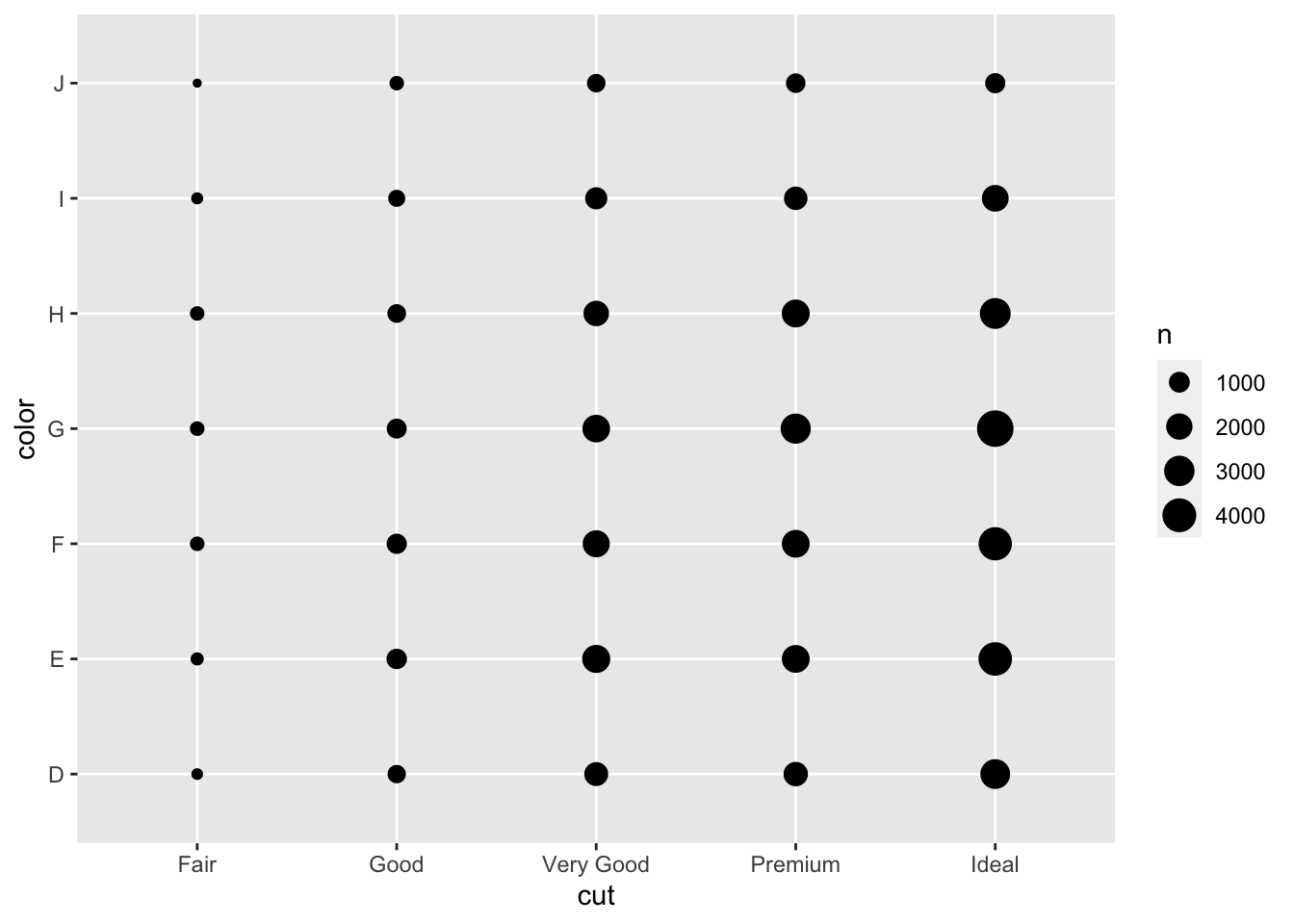
diamonds %>%
  count(color, cut)
## # A tibble: 35 x 3
## color cut n
## <ord> <ord> <int>
## 1 D Fair 163
## 2 D Good 662
## 3 D Very Good 1513
## 4 D Premium 1603
## 5 D Ideal 2834
## 6 E Fair 224
## 7 E Good 933
## 8 E Very Good 2400
## 9 E Premium 2337
## 10 E Ideal 3903
## # … with 25 more rowsdiamonds%>%count(color, cut)%>%
ggplot(mapping = aes(x=color, y=cut))+
geom_tile(aes(fill=n))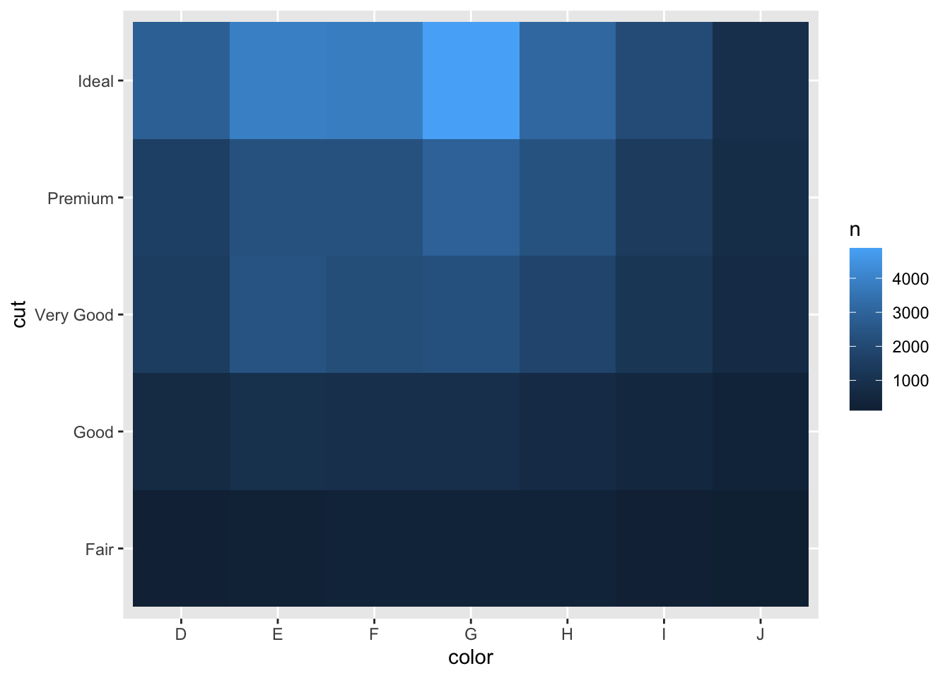
#two coutinuous variables
ggplot(data = diamonds)+
  geom_point(aes(x=carat, price))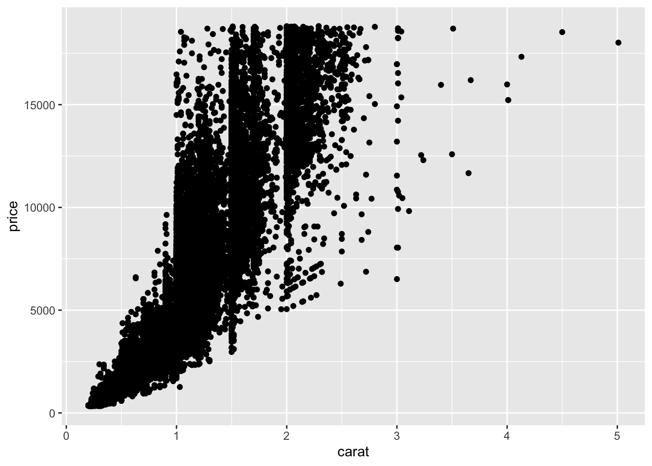
ggplot(data = diamonds)+
  geom_point(aes(x=carat, price),
             alpha=1/100)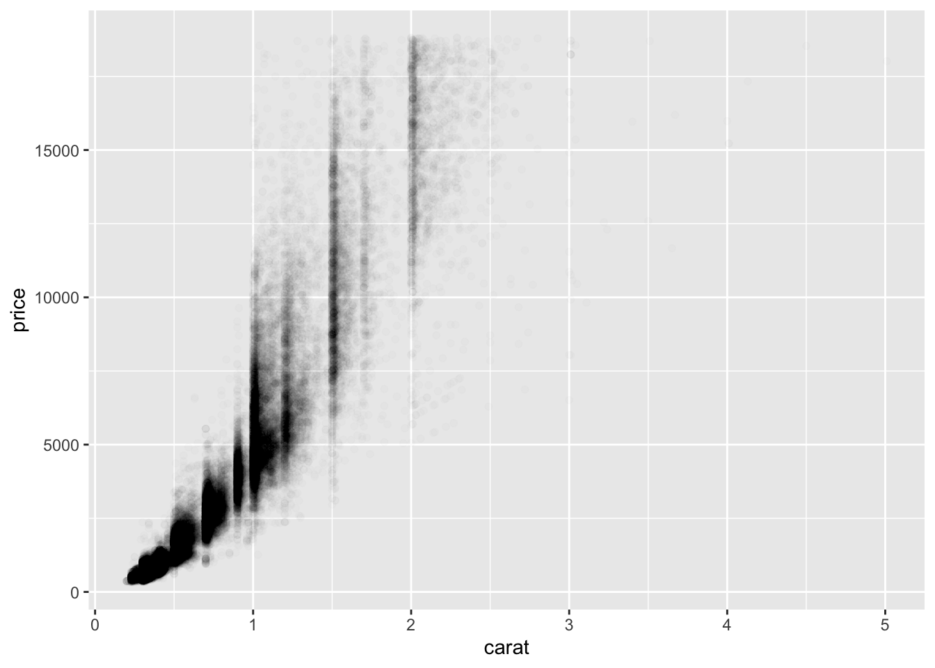
#use geom_bin2d() and hexbin() to bin into two dimensions
ggplot(data = smaller)+
  geom_bin2d(aes(carat, price))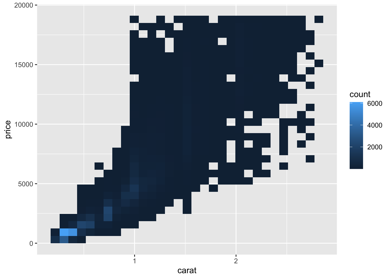
#install.packages("hexbin")
ggplot(data = smaller)+
  geom_hex(mapping = aes(carat, price))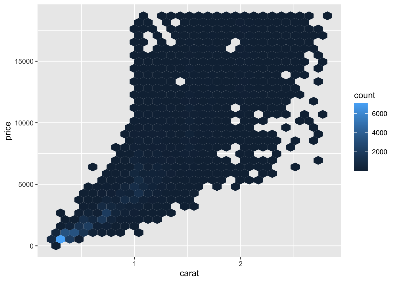
#boxplot
ggplot(smaller, aes(carat, price))+
         geom_boxplot(aes(group=cut_width(carat, .1)))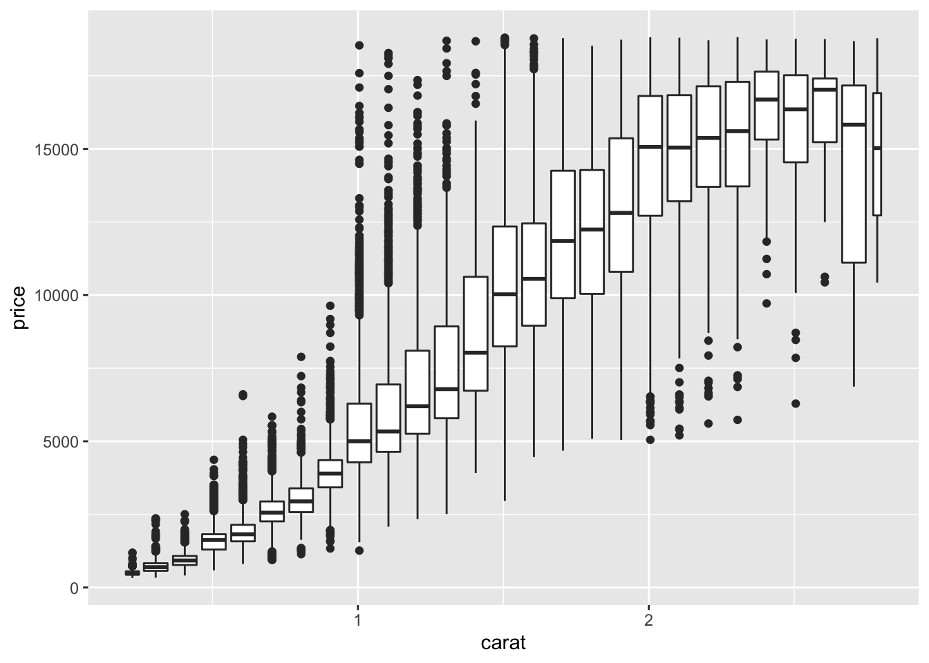
ggplot(smaller, aes(carat, price))+
  geom_boxplot(aes(group=cut_number(carat, 20)))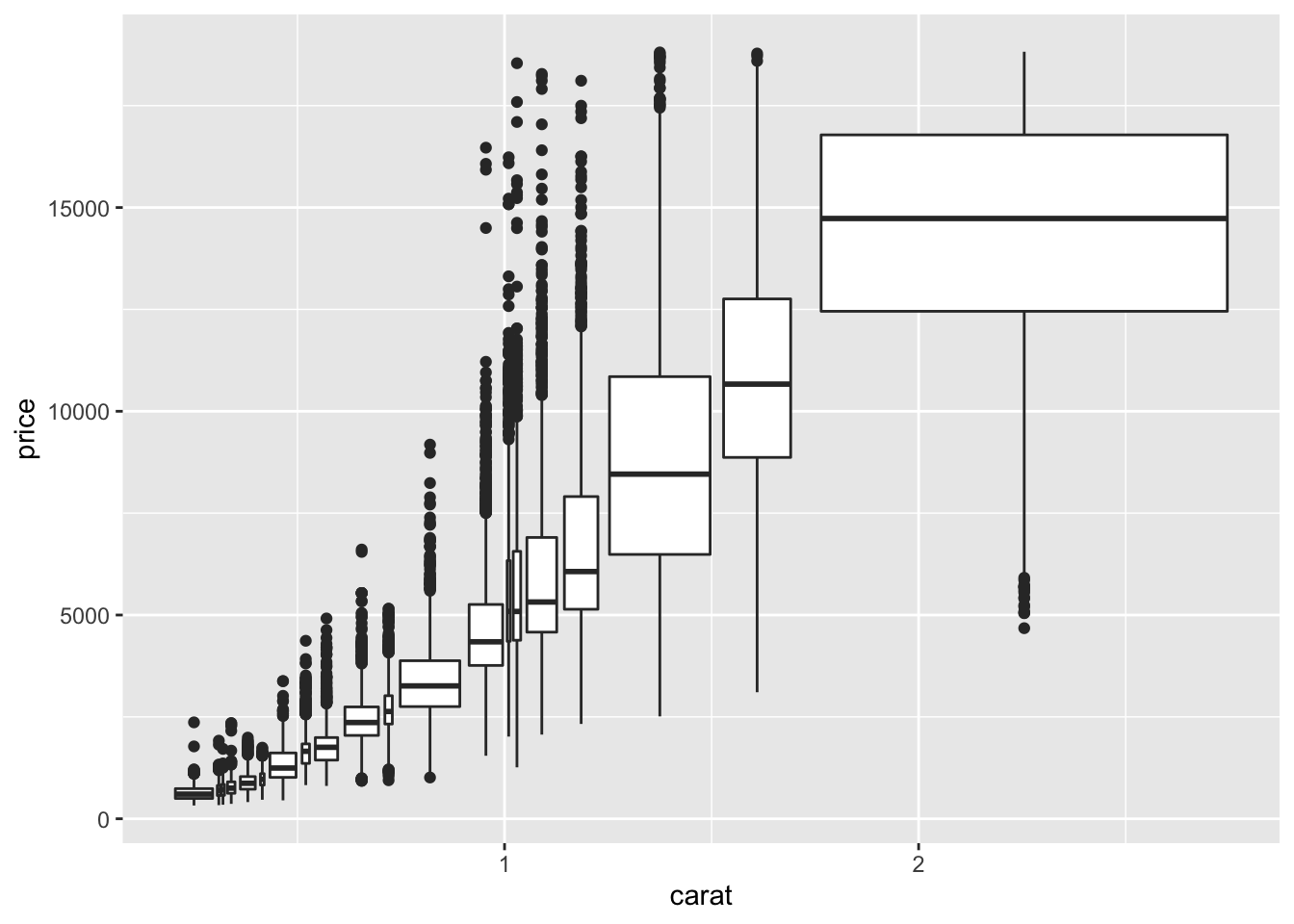
#an example of coord_cartesian() to zoom in
ggplot(diamonds)+
  geom_point(aes(x,y))+
  coord_cartesian(xlim = c(4,11), ylim = c(4,11))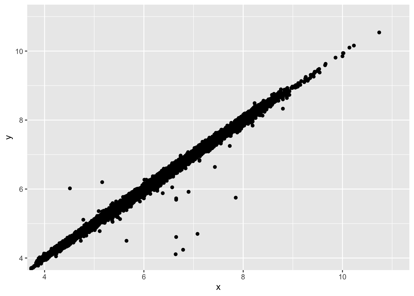
#patterns and models
ggplot(data = faithful)+
  geom_point(aes(eruptions, waiting))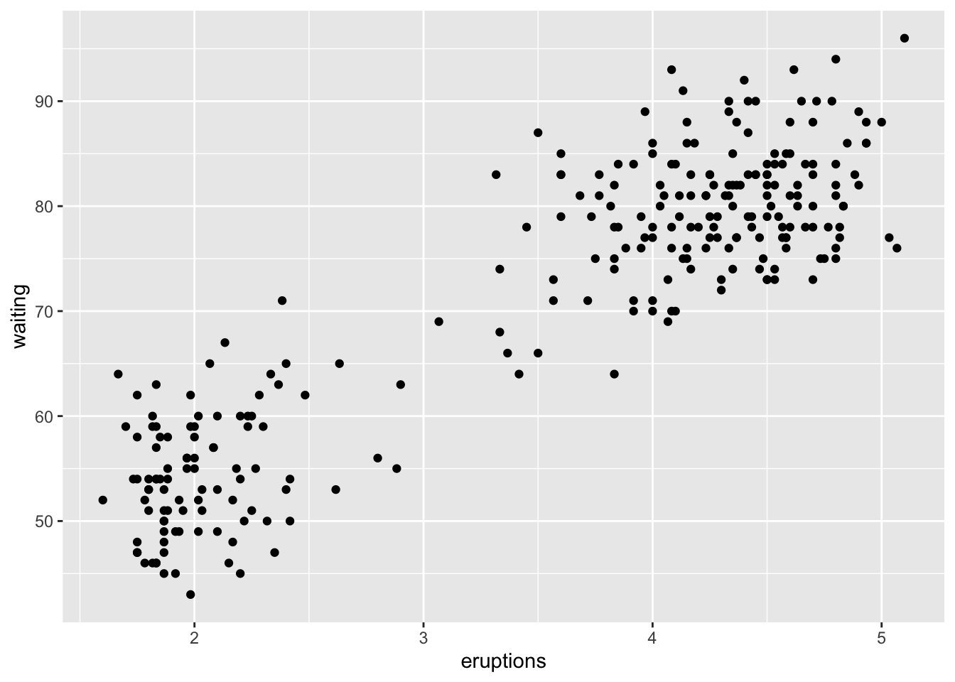
library(modelr)
mod <- lm(log(price)~log(carat), data = diamonds)
diamonds2 <- diamonds %>%
  add_residuals(mod)%>%
  mutate(resid=exp(resid))
ggplot(diamonds2)+
  geom_point(aes(carat, resid))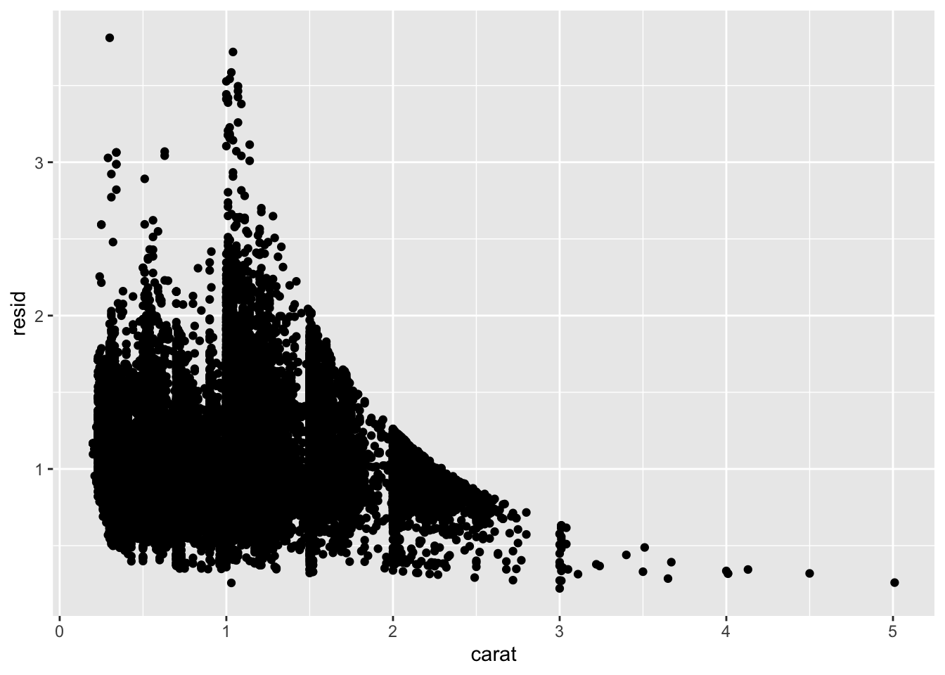
ggplot(data = diamonds2)+
  geom_boxplot(aes(cut, resid))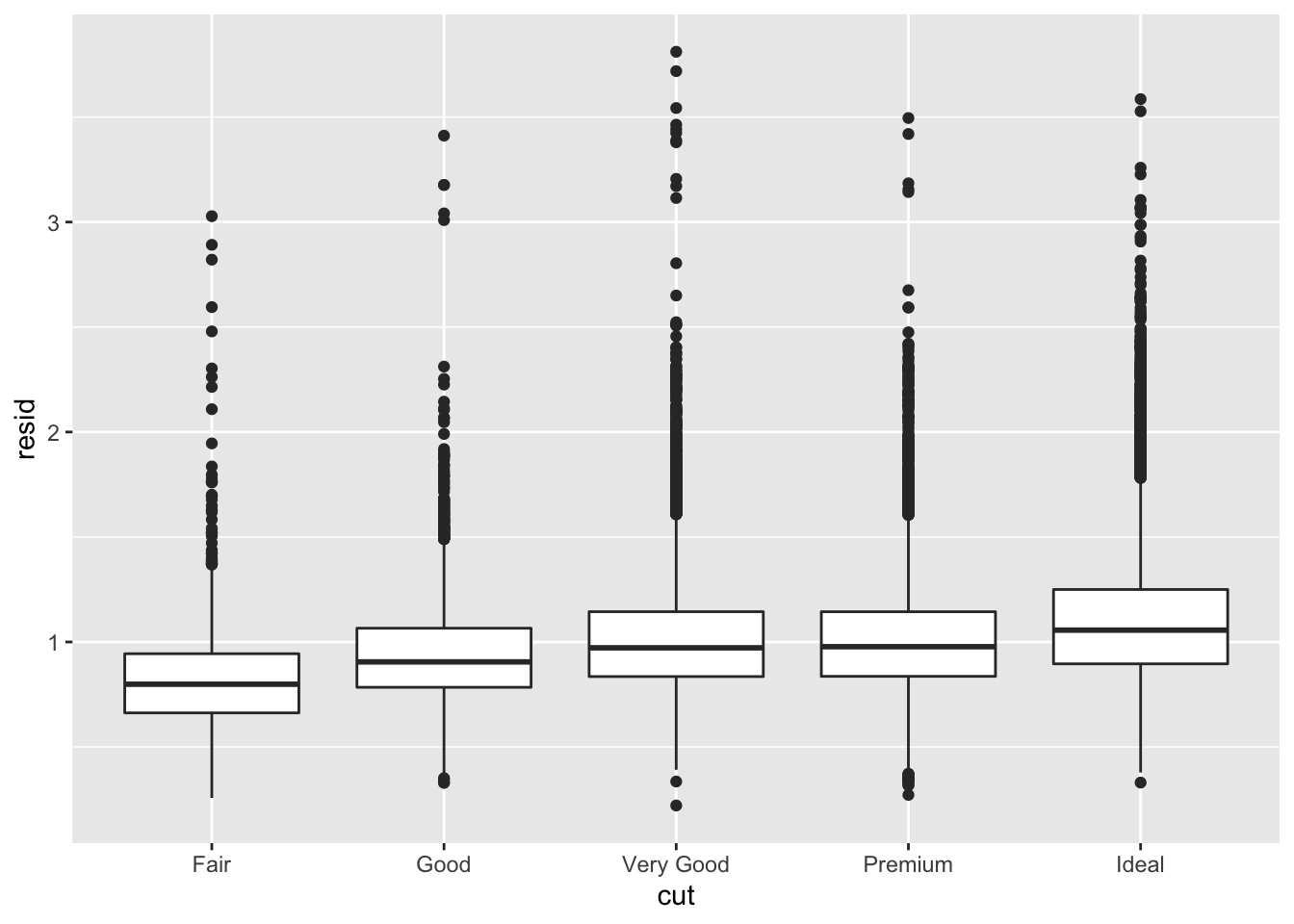
#relative to their size, better quality diamonds are more expensive