Chapter 2 ggplot2

2.1 introduction to ggplot2 from Wickham and Grolemund' chapter 1

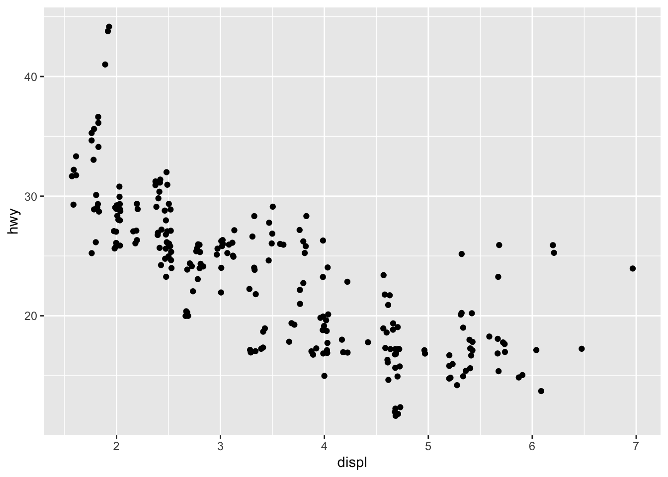
#scatterplot
#build coordinate system at global level, and geom_ function at local level
library(ggplot2)
ggplot(data = mpg)+
  geom_point(mapping = aes(x=displ, y=hwy))

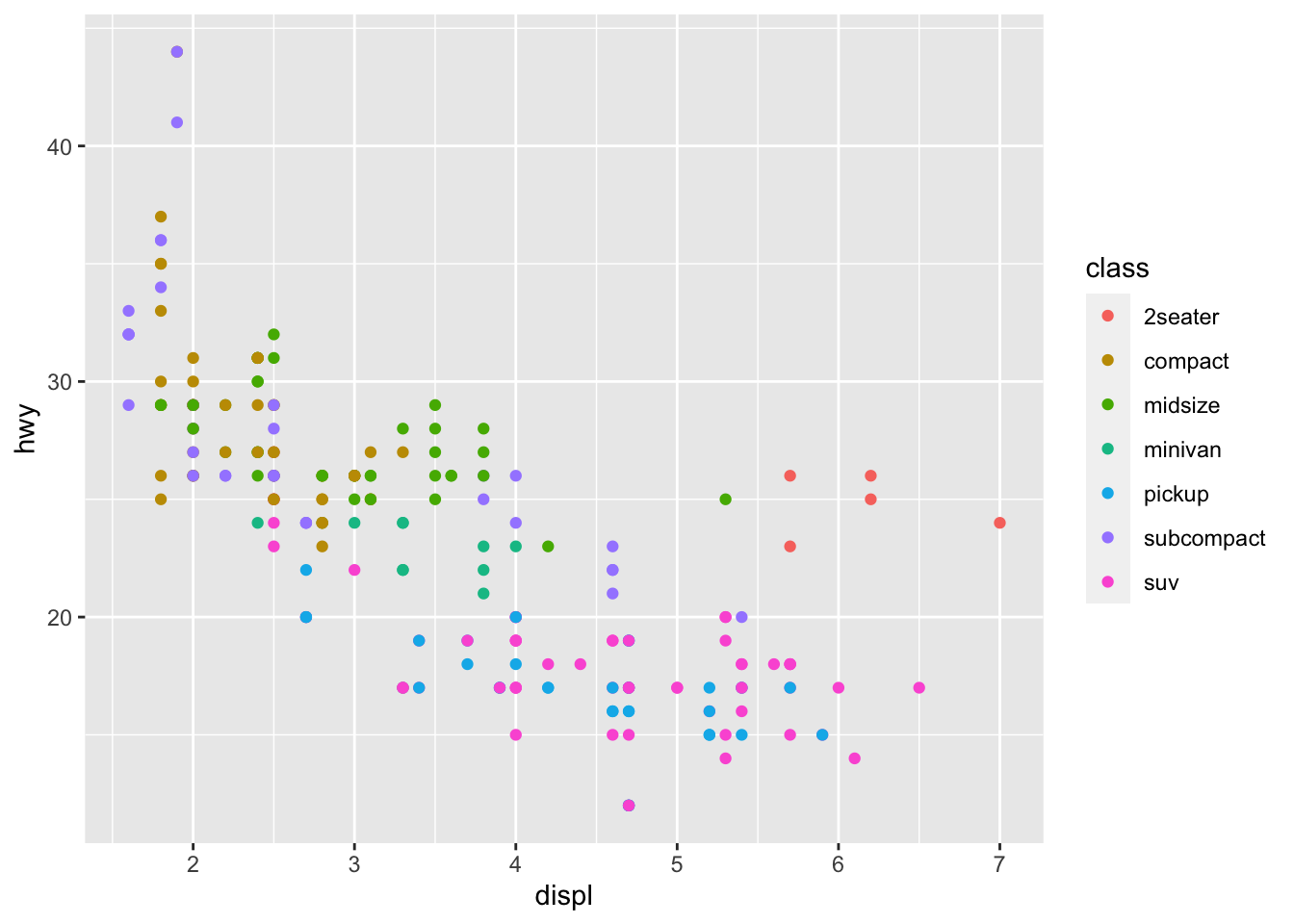
g <- ggplot(data = mpg)
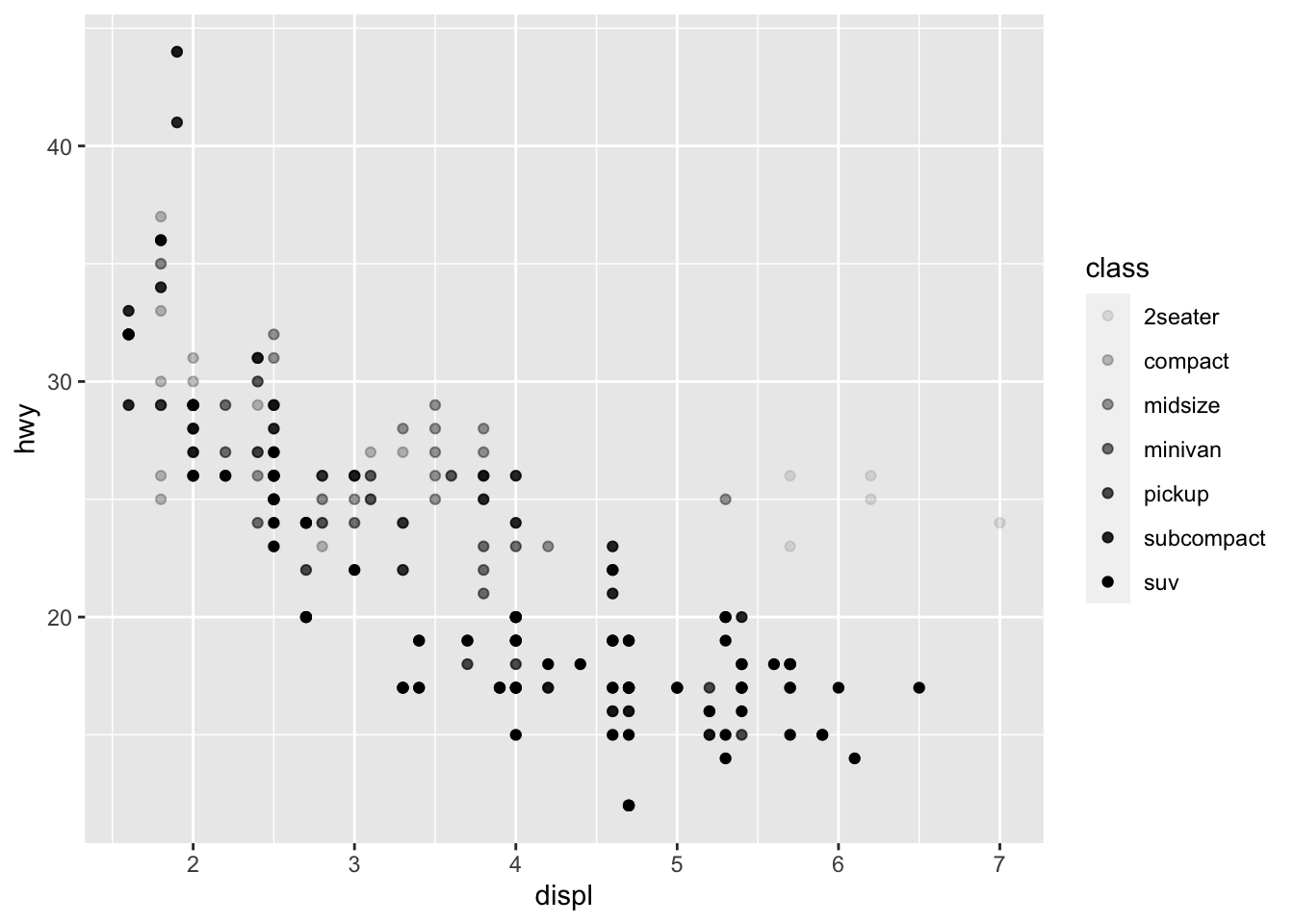
g+geom_point(mapping = aes(x=displ, y=hwy, color=class))

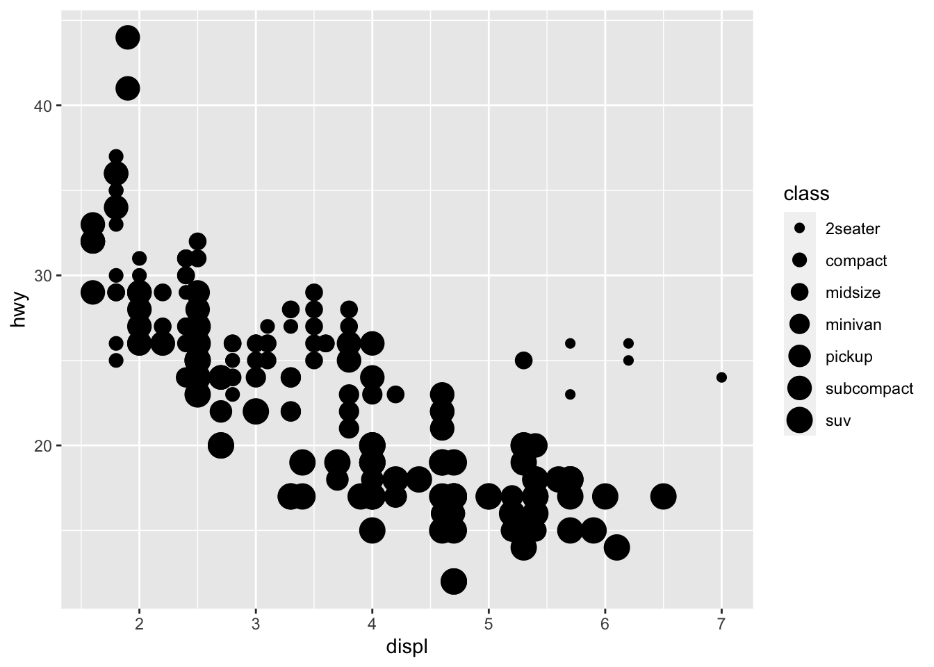
g+geom_point(aes(x=displ, y=hwy, size=class))

## Warning: Using size for a discrete variable is not advised.

g+geom_point(aes(x=displ, y=hwy, alpha=class))

## Warning: Using alpha for a discrete variable is not advised.

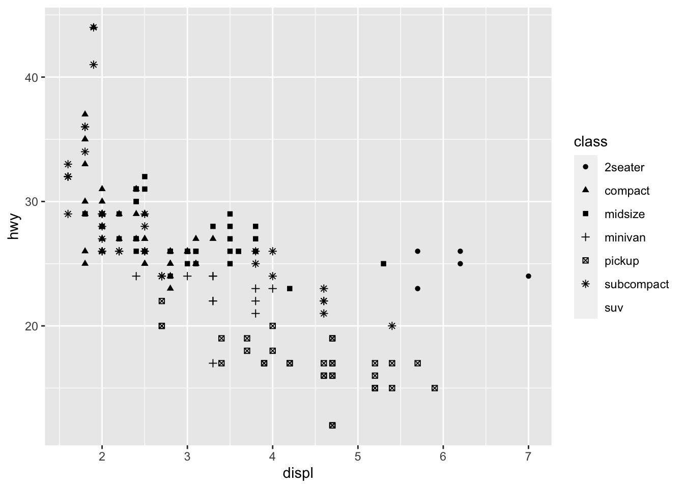
g+geom_point(aes(x=displ, y=hwy, shape=class)) #the 7th category is not plotted

## Warning: The shape palette can deal with a maximum of 6 discrete values because more than 6 becomes difficult to
## discriminate; you have 7. Consider specifying shapes manually if you must have them.

## Warning: Removed 62 rows containing missing values (geom_point).

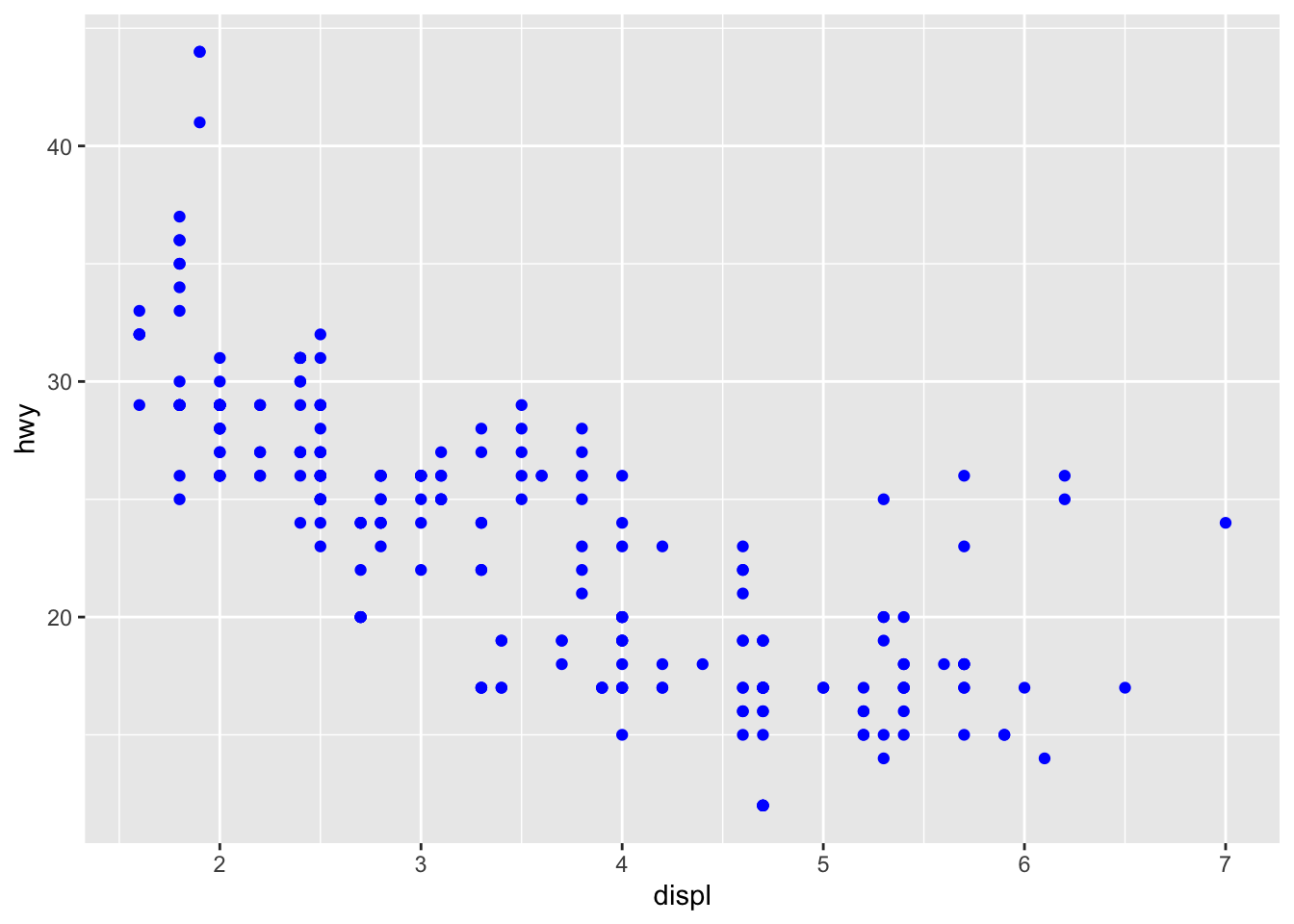
g+geom_point(aes(x=displ, y=hwy), color="blue")

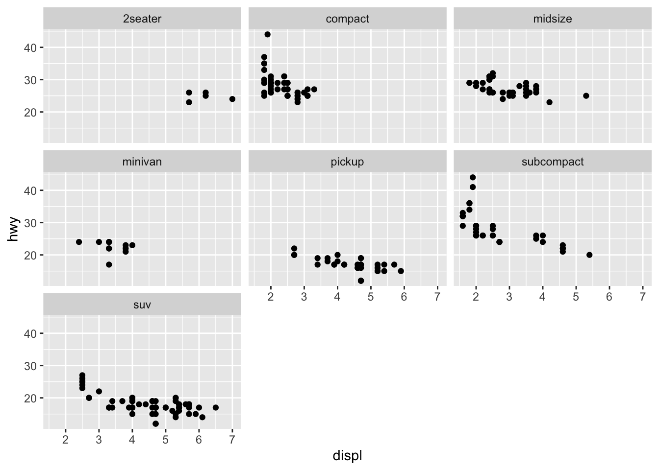
#facets
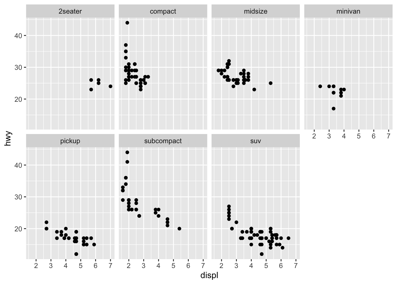
g+geom_point(aes(x=displ, y=hwy))+
  facet_wrap(~class, nrow=2)

g+geom_point(aes(x=displ, y=hwy))+
  facet_wrap(~class) #by default nrow=3

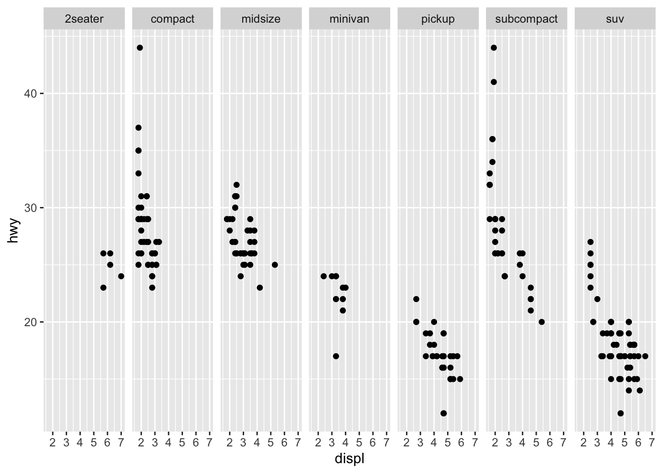
g+geom_point(aes(x=displ, y=hwy))+
  facet_grid(~class)

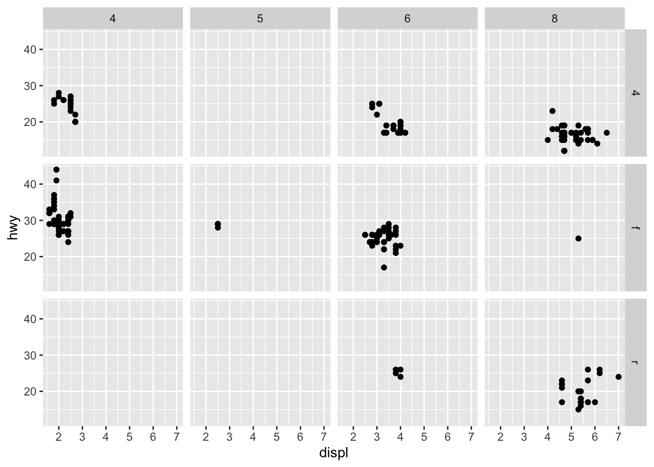
g+geom_point(aes(x=displ, y=hwy))+
  facet_grid(drv ~ cyl)

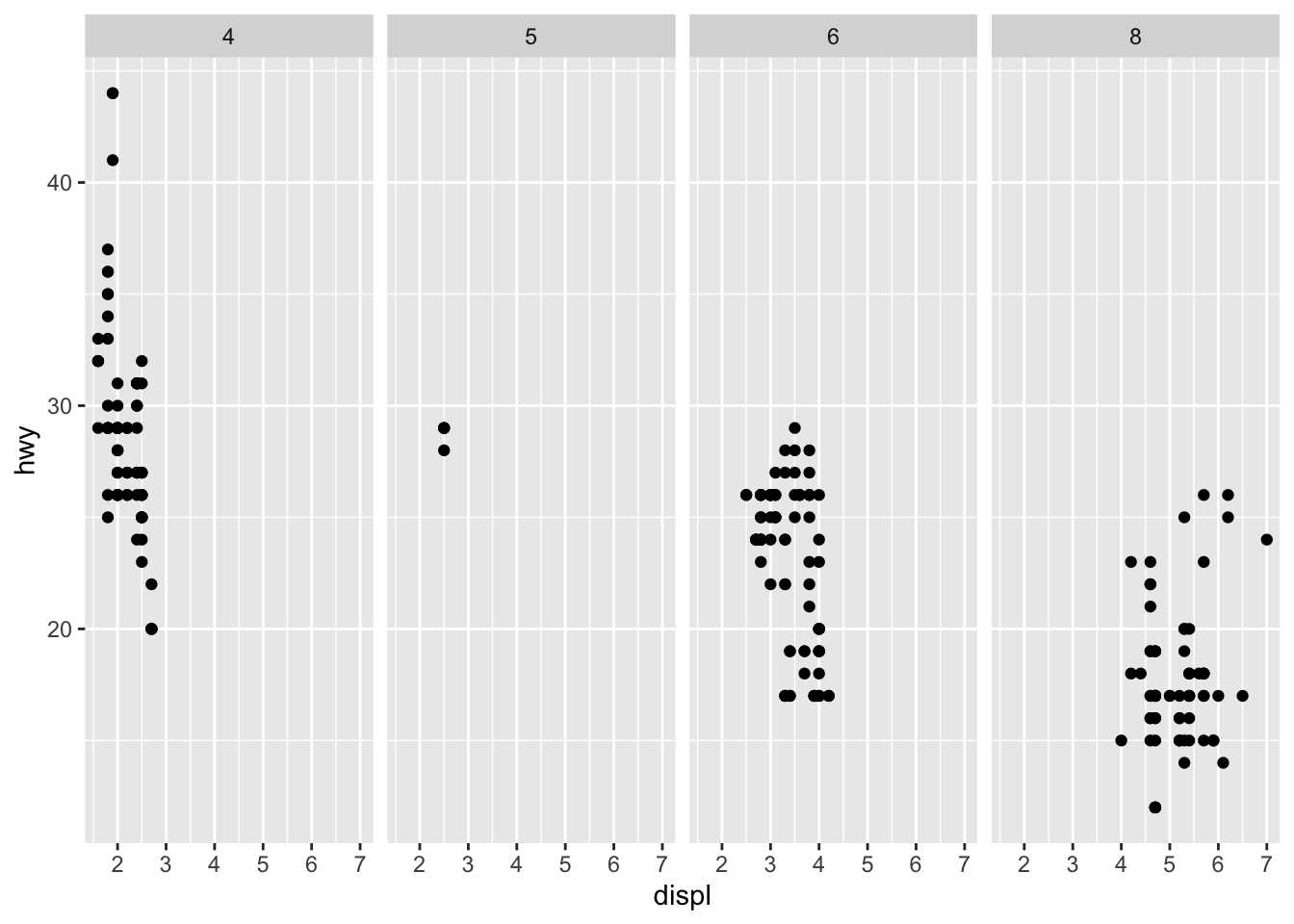
g+geom_point(aes(x=displ, y=hwy))+
  facet_grid(. ~ cyl)

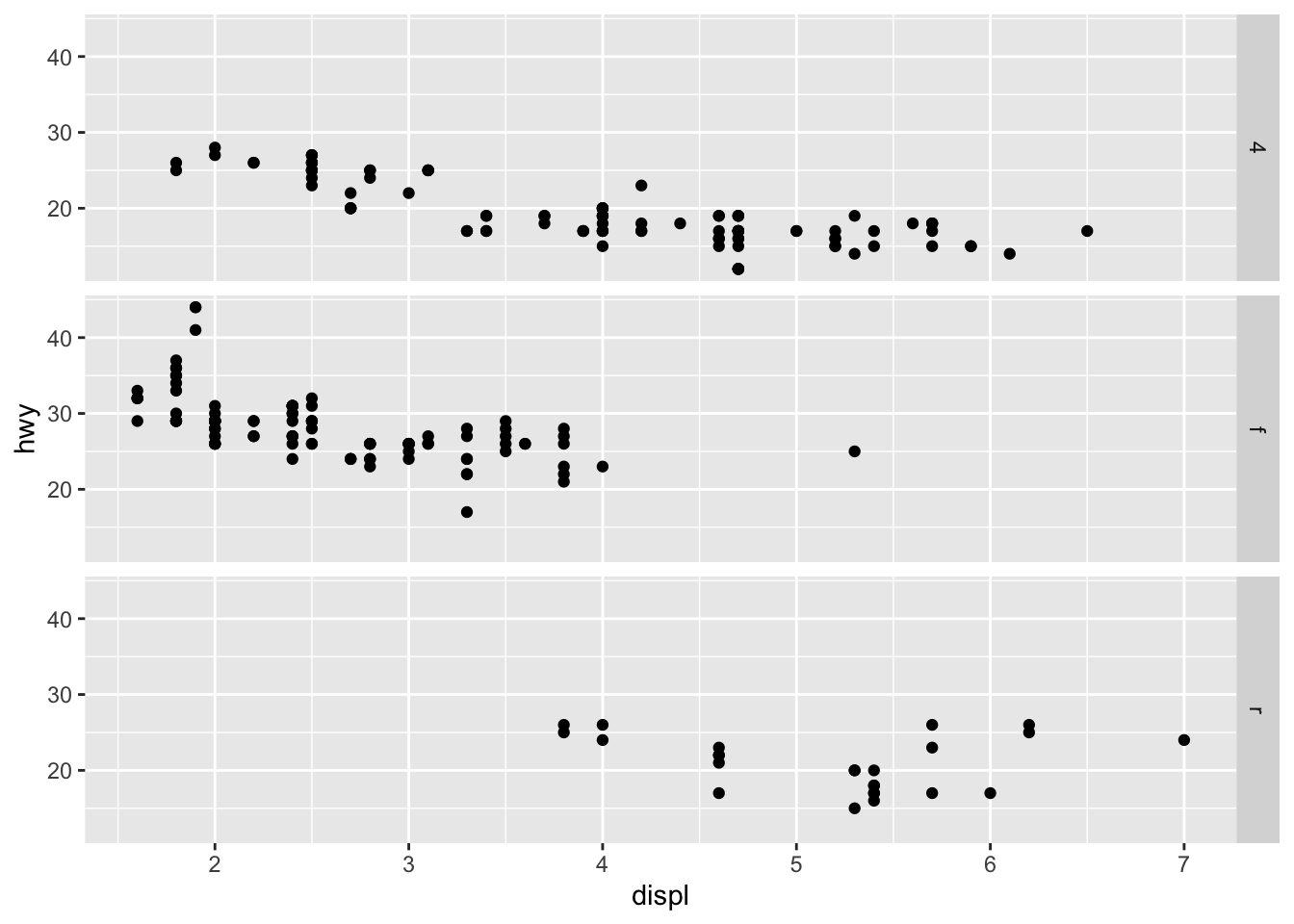
g+geom_point(aes(x=displ, y=hwy))+
  facet_grid(drv ~ .)

g+geom_point(aes(x=displ, y=hwy))+
  facet_wrap(drv ~ .)

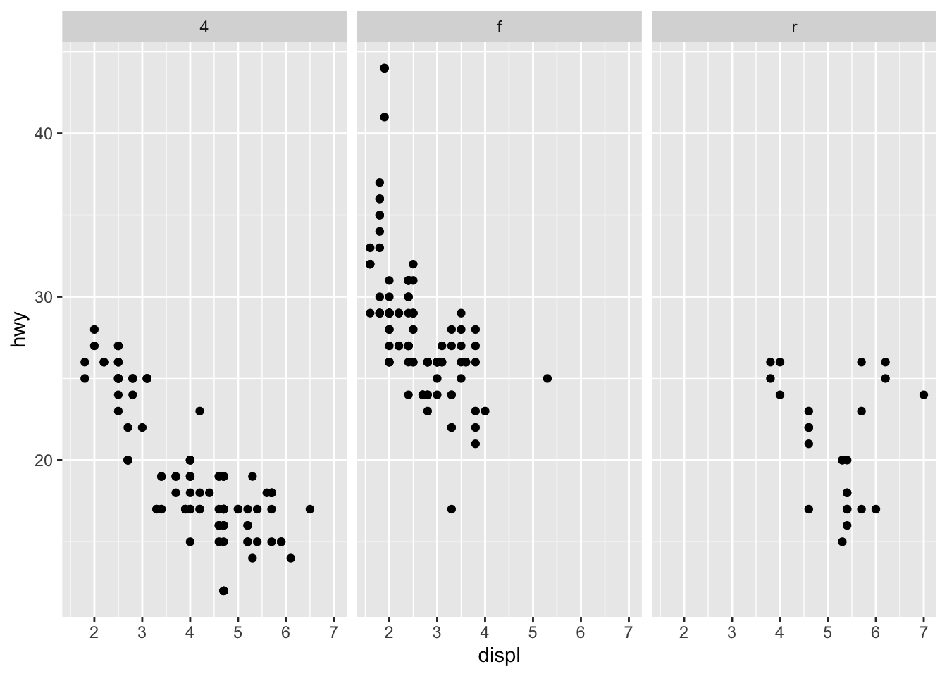
g+geom_point(aes(x=displ, y=hwy))+
  facet_grid(. ~ drv)

#lines (use of group, color, and linetype)
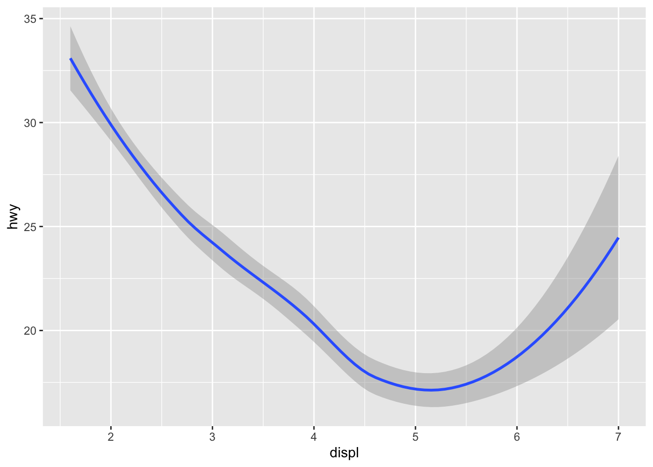
#by default, geom_smooth use method="loess"
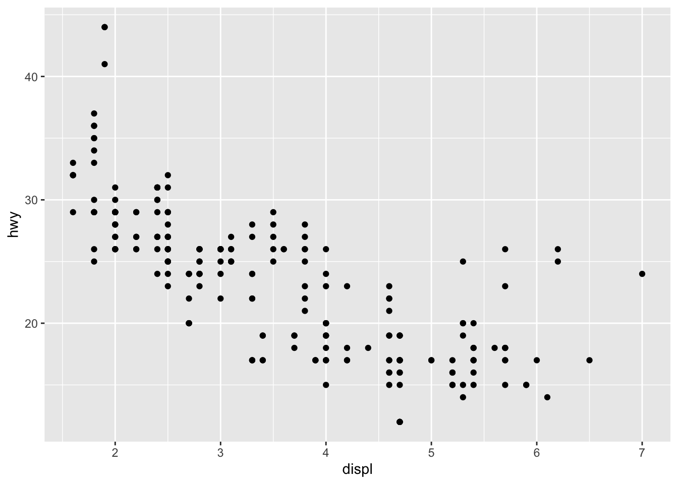
g+geom_point(aes(x=displ, y=hwy))

g+geom_smooth(aes(x=displ, y=hwy))

## `geom_smooth()` using method = 'loess' and formula 'y ~ x'

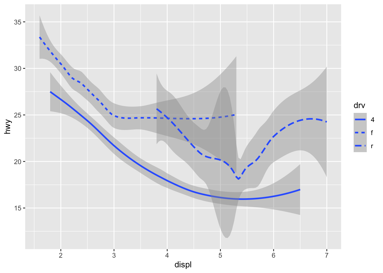
g+geom_smooth(aes(x=displ, y=hwy, linetype=drv)) #with legend

## `geom_smooth()` using method = 'loess' and formula 'y ~ x'

g+geom_point(aes(x=displ, y=hwy))+
  geom_smooth(aes(x=displ, y=hwy))

## `geom_smooth()` using method = 'loess' and formula 'y ~ x'

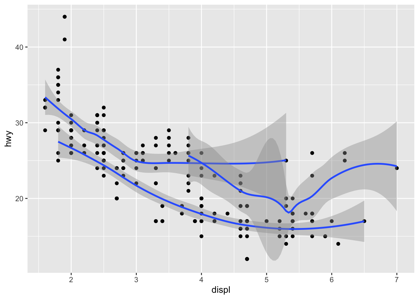
g+geom_point(aes(x=displ, y=hwy))+
  geom_smooth(aes(x=displ, y=hwy, group=drv),
              show.legend = T) #do not add legend

## `geom_smooth()` using method = 'loess' and formula 'y ~ x'

#local level
#g+geom_point(aes(x=displ, y=hwy))+
#  geom_smooth(aes(group=drv),
#              show.legend = T)

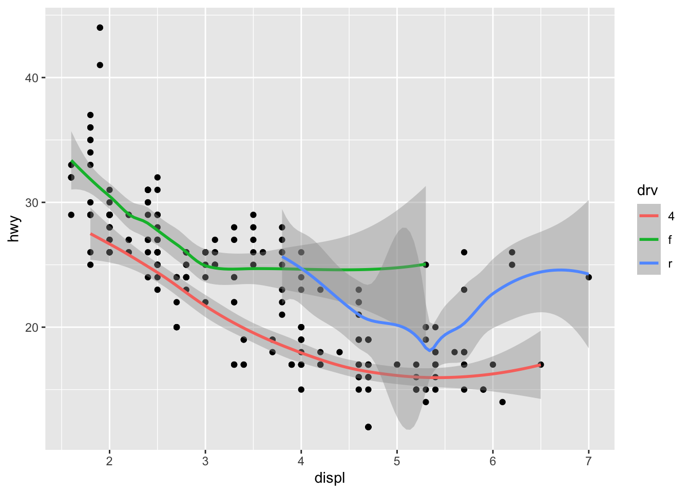
g+geom_point(aes(x=displ, y=hwy))+
  geom_smooth(aes(x=displ, y=hwy, color=drv),
              show.legend = T)

## `geom_smooth()` using method = 'loess' and formula 'y ~ x'

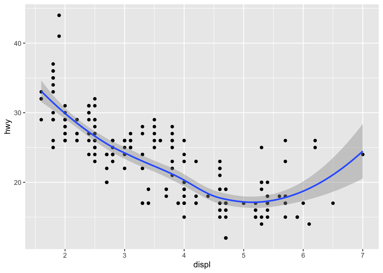
g <- ggplot(data = mpg, mapping = aes(x=displ, y=hwy))
g+geom_point()+geom_smooth()

## `geom_smooth()` using method = 'loess' and formula 'y ~ x'

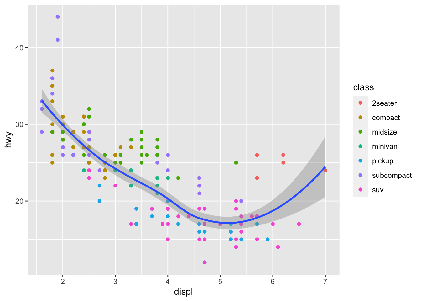
g+geom_point(aes(color=class))+geom_smooth()

## `geom_smooth()` using method = 'loess' and formula 'y ~ x'

#g+geom_point(aes(color=class))+geom_smooth(
#  data = filter(mpg, class=="subcompact"),
#  se=FALSE,
#  method = "lm"
#)

ggplot(data = diamonds)+
  stat_count(mapping = aes(x=cut))

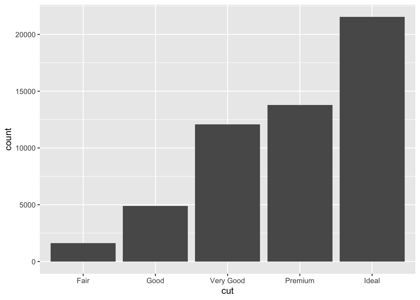
ggplot(data = diamonds)+
  geom_bar(mapping = aes(x=cut))

#ggplot(data = diamonds)+
#  geom_histogram(mapping = aes(x=cut))#do not work; x needs to be a continuous variable
ggplot(data = diamonds)+
  geom_histogram(mapping = aes(x=cut), stat = "count") 

## Warning: Ignoring unknown parameters: binwidth, bins, pad

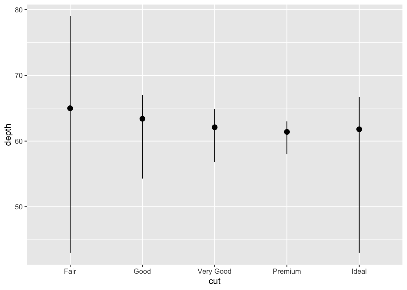
ggplot(data = diamonds)+
  stat_summary(mapping = aes(x=cut, y=depth),
               fun.ymax = max,
               fun.ymin = min,
               fun.y = median)

## Warning: `fun.y` is deprecated. Use `fun` instead.

## Warning: `fun.ymin` is deprecated. Use `fun.min` instead.

## Warning: `fun.ymax` is deprecated. Use `fun.max` instead.

?stat_summary

#position adjustments
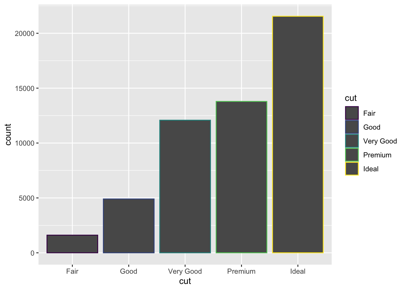
ggplot(data = diamonds)+
  geom_bar(mapping = aes(x=cut, color=cut))

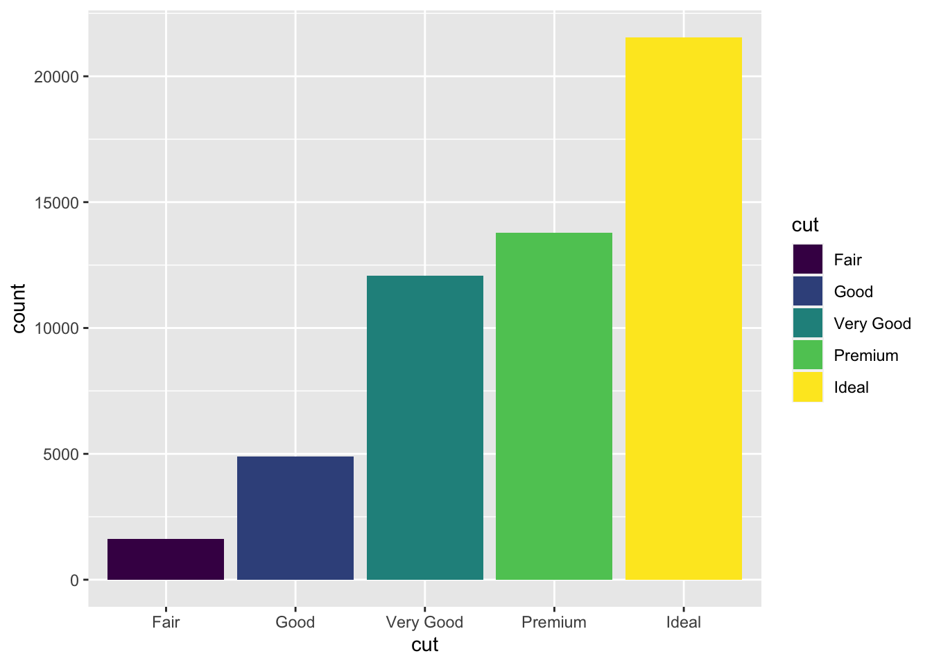
ggplot(data = diamonds)+
  geom_bar(mapping = aes(x=cut, fill=cut))

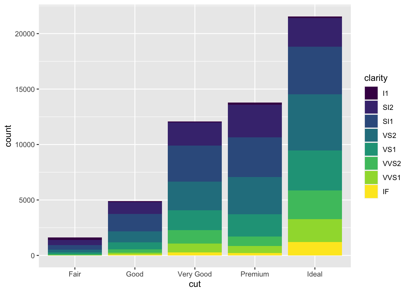
ggplot(data = diamonds)+
  geom_bar(mapping = aes(x=cut, fill=clarity))

#position
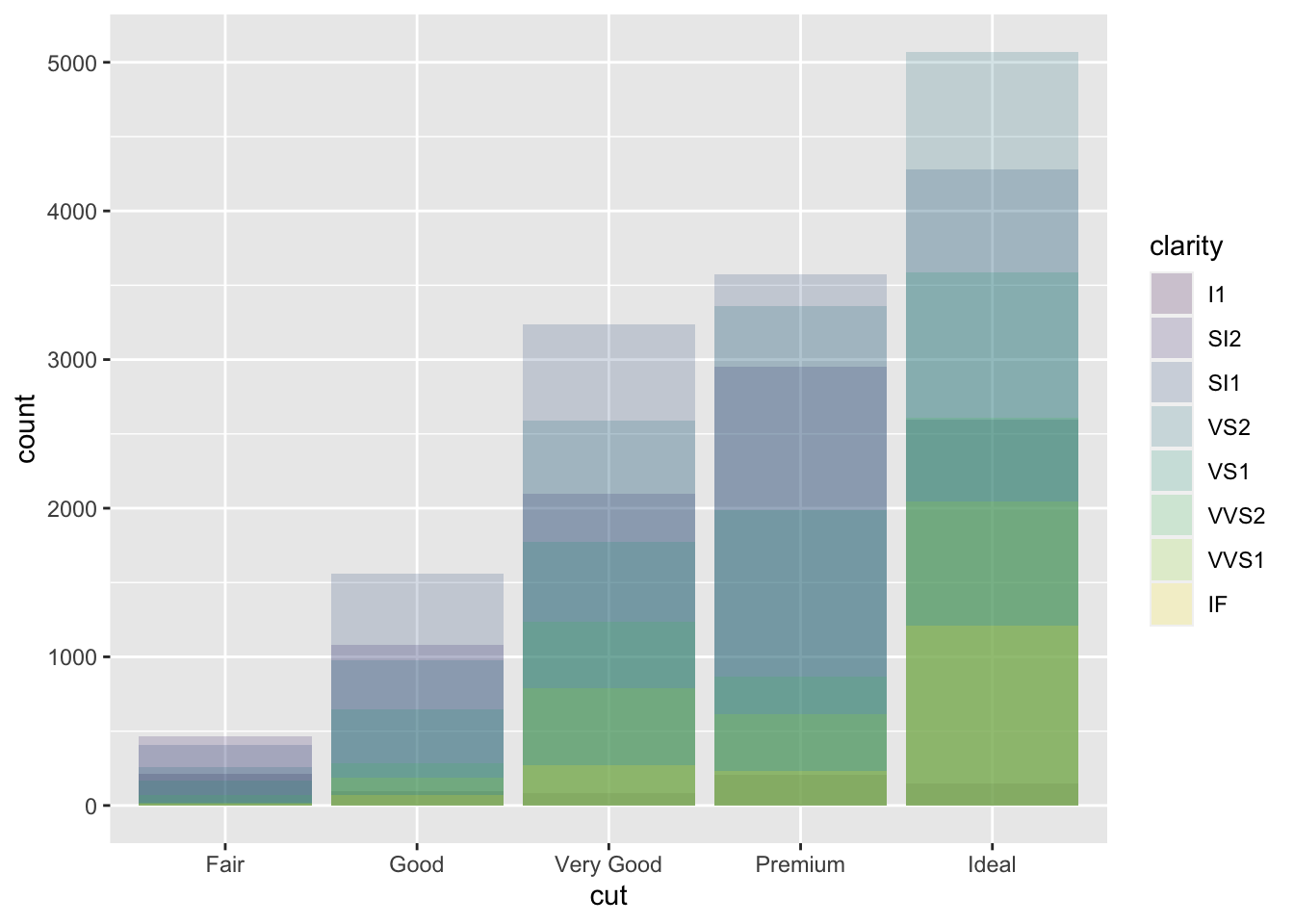
ggplot(data = diamonds,
       mapping = aes(x=cut, fill=clarity))+
  geom_bar(alpha=1/5, position = "identity")

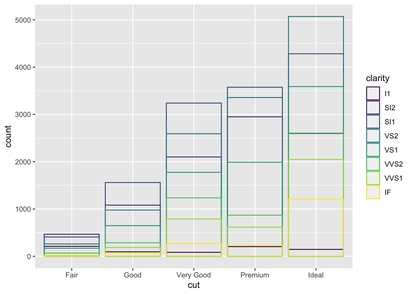
ggplot(data = diamonds,
       mapping = aes(x=cut, color=clarity))+
  geom_bar(fill=NA, position = "identity")

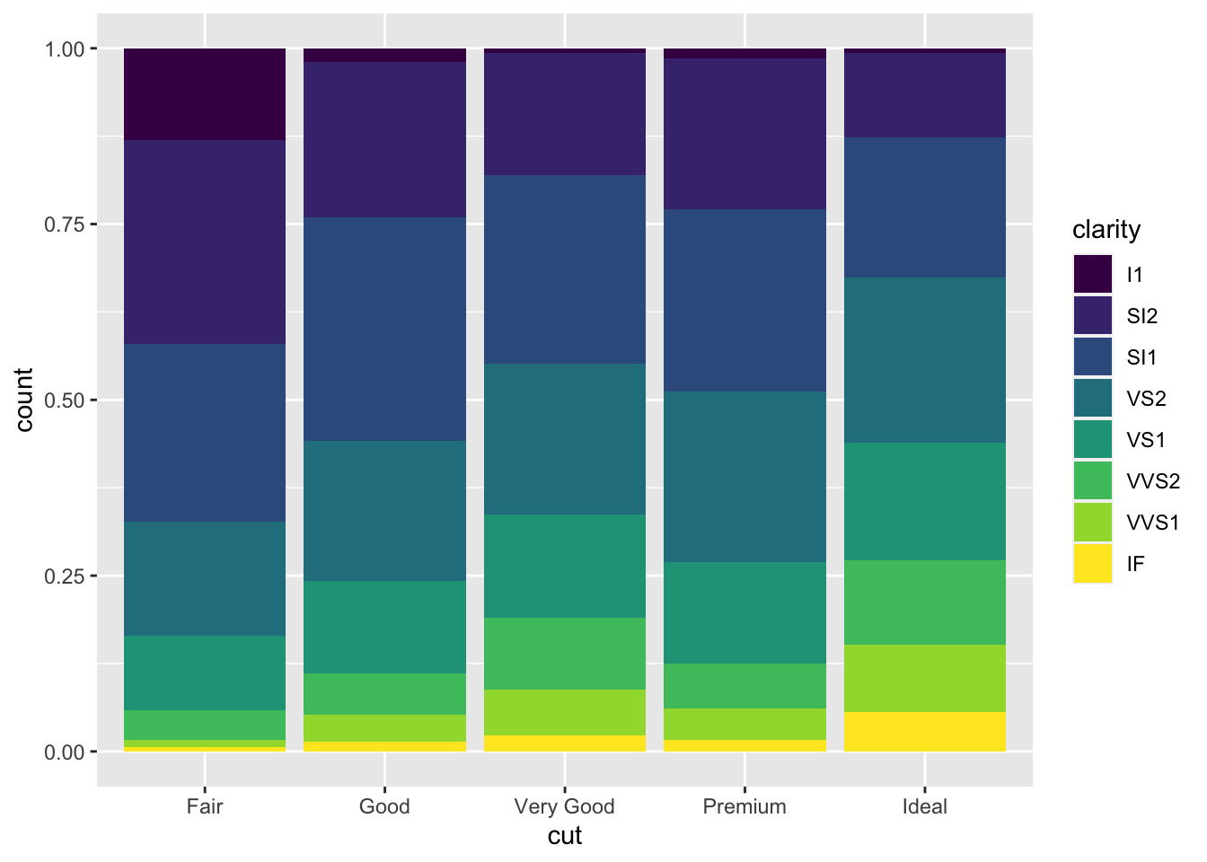
#position=fill - stacking
ggplot(data = diamonds)+
       geom_bar(mapping = aes(x=cut, fill=clarity),
                position = "fill")

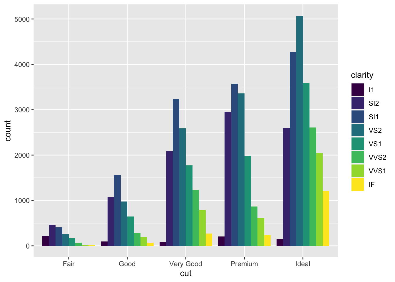
#dodge-besides each other
ggplot(data = diamonds)+
  geom_bar(mapping = aes(x=cut, fill=clarity),
           position = "dodge")

#add some random noise
table(mpg$displ)

## 
## 1.6 1.8 1.9   2 2.2 2.4 2.5 2.7 2.8   3 3.1 3.3 3.4 3.5 3.6 3.7 3.8 3.9   4 4.2 4.4 4.6 4.7   5 5.2 5.3 5.4 5.6 5.7 5.9 
##   5  14   3  21   6  13  20   8  10   8   6   9   4   5   2   3   8   3  15   4   1  11  17   2   5   6   8   1   8   2 
##   6 6.1 6.2 6.5   7 
##   1   1   2   1   1

ggplot(data = mpg)+
  geom_point(mapping = aes(x=displ, y=hwy),
             position = "jitter")

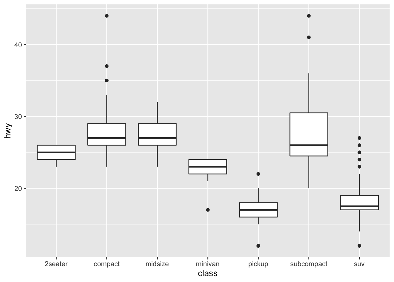
#coordinate system
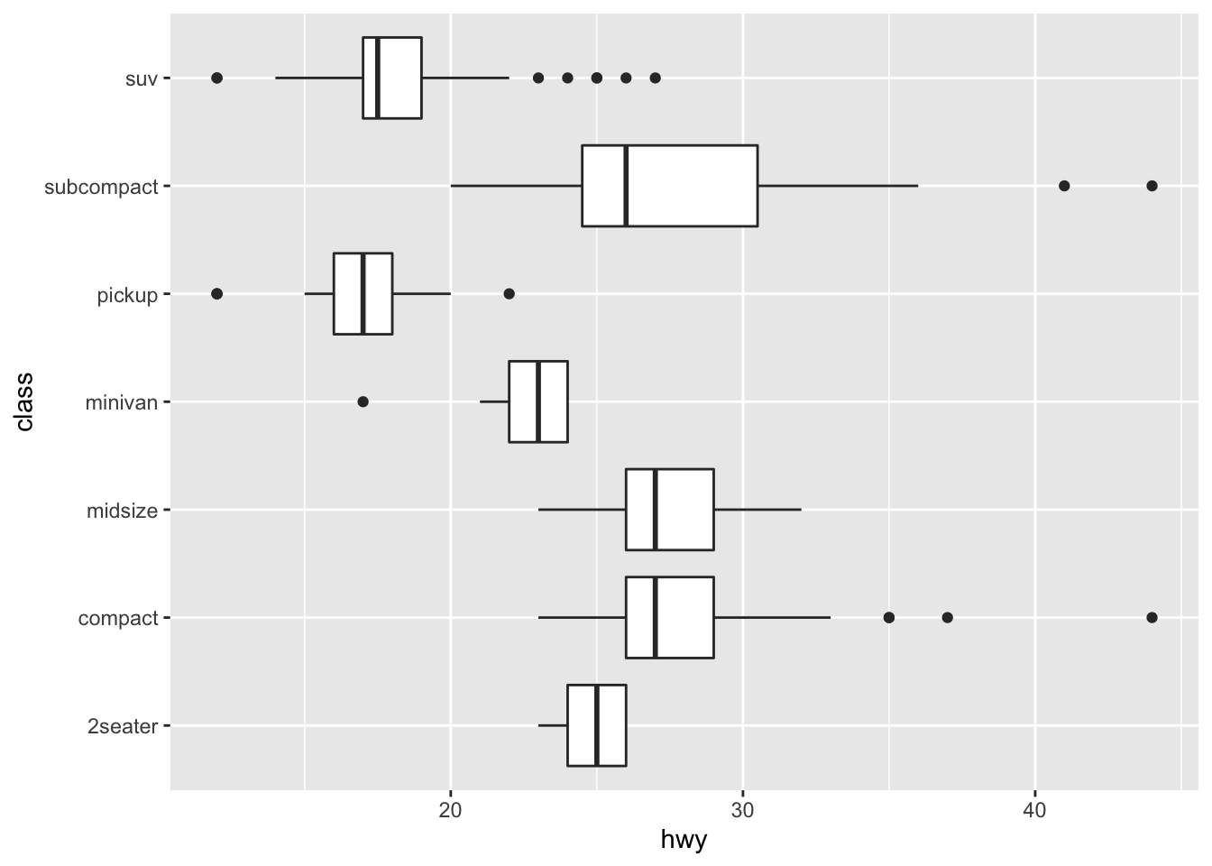
ggplot(data = mpg, mapping = aes(x=class, y=hwy))+
  geom_boxplot()

ggplot(data = mpg, mapping = aes(x=class, y=hwy))+
  geom_boxplot()+
  coord_flip()

nz<- map_data("nz")
ggplot(nz, aes(long, lat, group=group))+
  geom_polygon(fill="white", color="black")

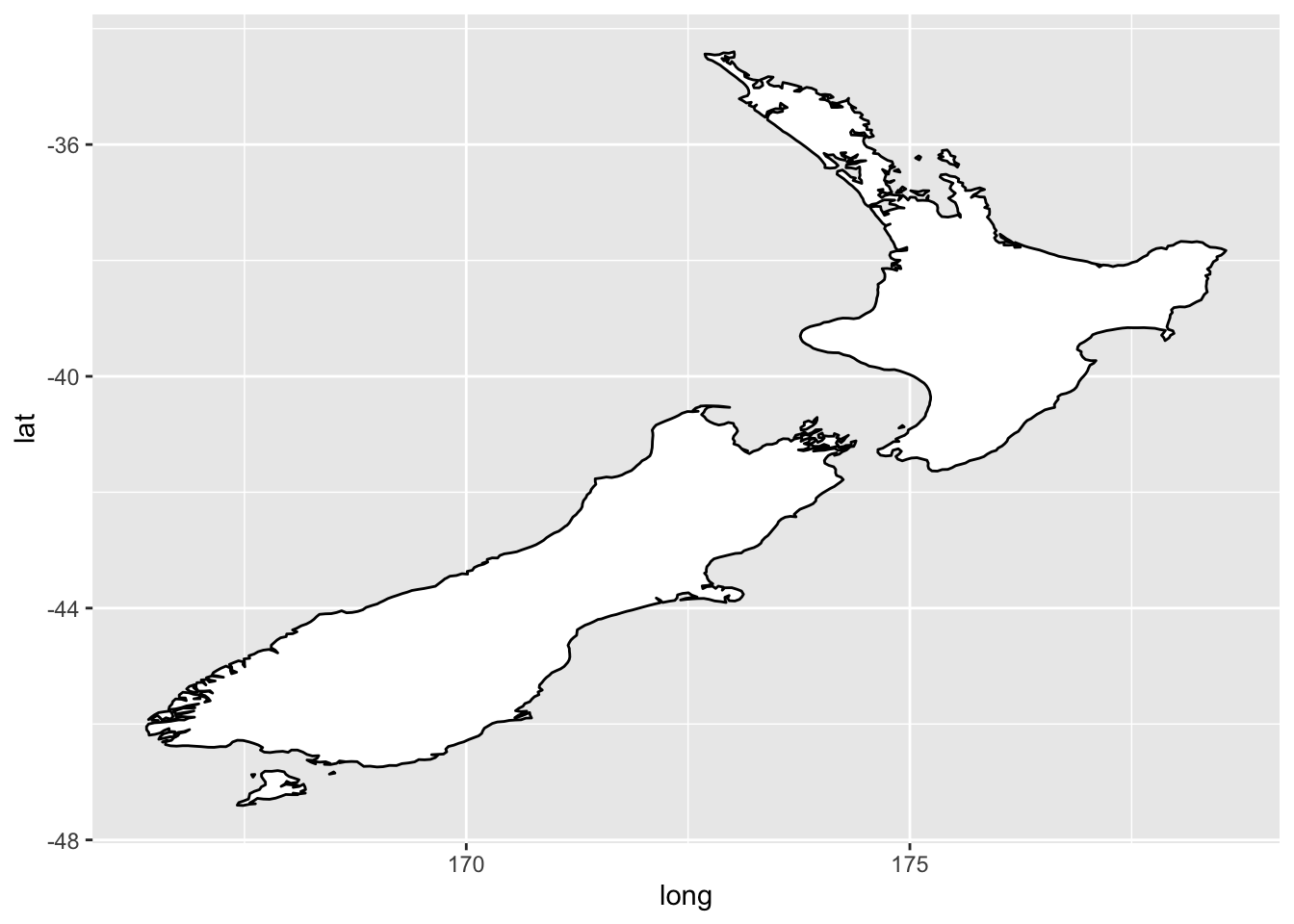
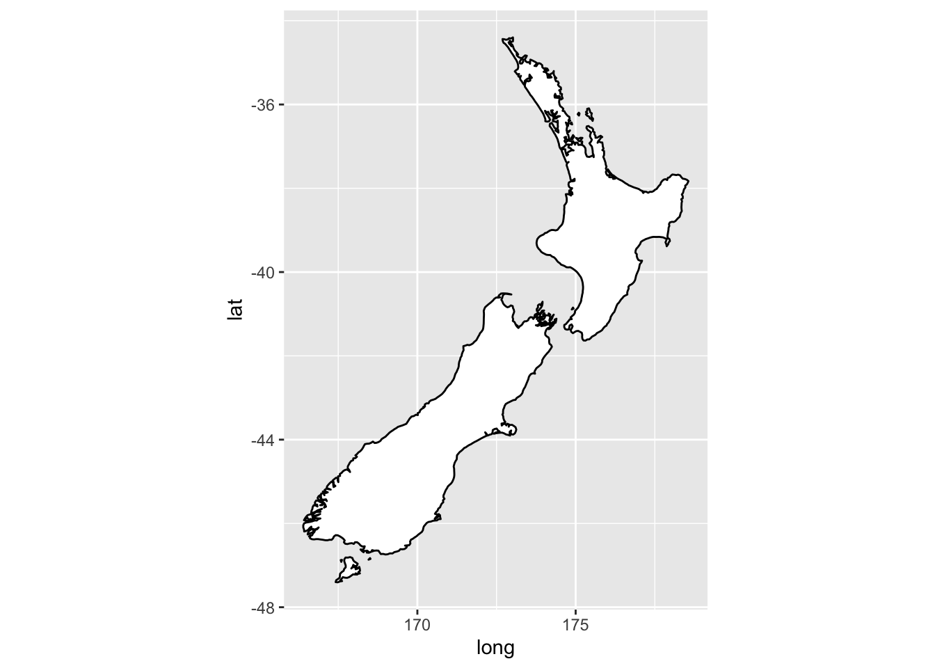
#coord_quickmap() sets the aspect ratio correctly
ggplot(nz, aes(long, lat, group=group))+
  geom_polygon(fill="white", color="black")+
  coord_quickmap()

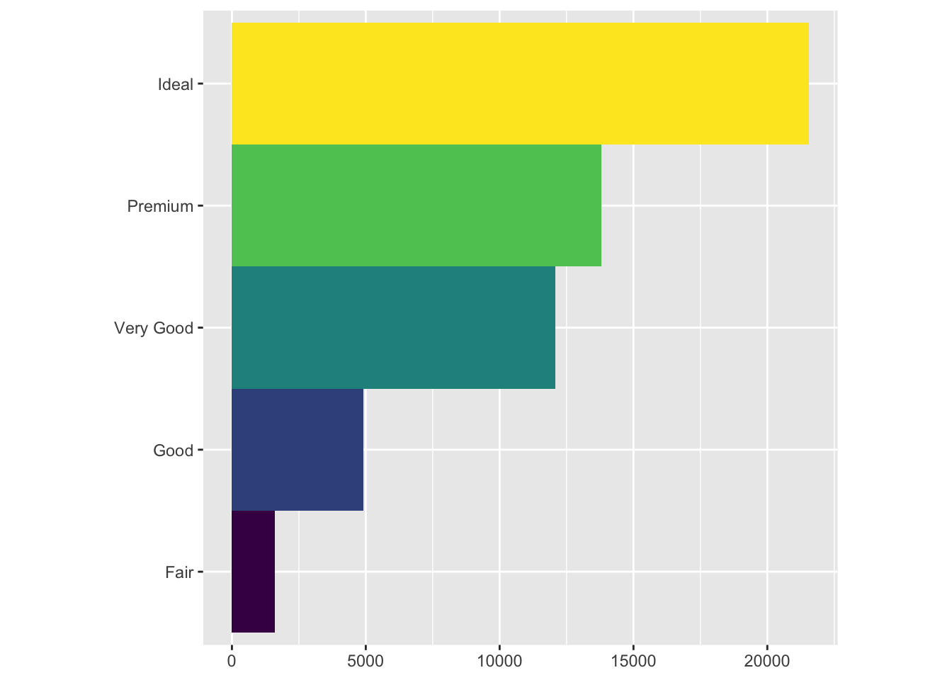
bar <- ggplot(data = diamonds)+
  geom_bar(mapping = aes(x=cut, fill=cut),
           show.legend = F, #don't add legend
           width = 1)+
  theme(aspect.ratio = 1)+
  labs(x=NULL, y=NULL) #don't add anything on x,y-axis
bar+coord_flip()

bar+coord_polar()