Chapter 8 Neural Networks in Time Series Analysis
# preamble setting the directories and loading packages
rm(list = ls())
setwd("C:/Users/Tejendra/Desktop/FoldersOnDesktop/UdemyCourse/Section7")
require(tidyverse)
require(tidymodels)
require(data.table)
require(tidyposterior)
require(tsibble)  #tsibble for time series based on tidy principles
require(fable)  #for forecasting based on tidy principles
require(ggfortify)  #for plotting timeseries
require(forecast)  #for forecast function
require(tseries)
require(chron)
require(lubridate)
require(directlabels)
require(zoo)
require(lmtest)
require(TTR)  #for smoothing the time series
require(MTS)
require(vars)
require(fUnitRoots)
require(lattice)
require(grid)
NNAR-Neural Network Autoregression Model- has two components, \(p \ \& \ k\). \(p\) denotes the number of lagged values that are used as inputs. \(k\) denotes the number of hidden nodes that are present. Output is denoted by \(NNAR(p, k)\). If the dataset is seasonal then also the notation is pretty similar, i.e., \(NNAR(p, P, k)\) where \(P\) denotes the number of seasonal lags. \(p\) is choosen based on the information criterion, like AIC. Neural nets has inherent random component. Therefore, it is suggested that the neural net model is run several times, 20 is the minimum requirement. Final result is then presented as mean or median. Also neural nets are known to not work well with the trend data. We should therefore, de-trend or differnce the data before running neural net model.
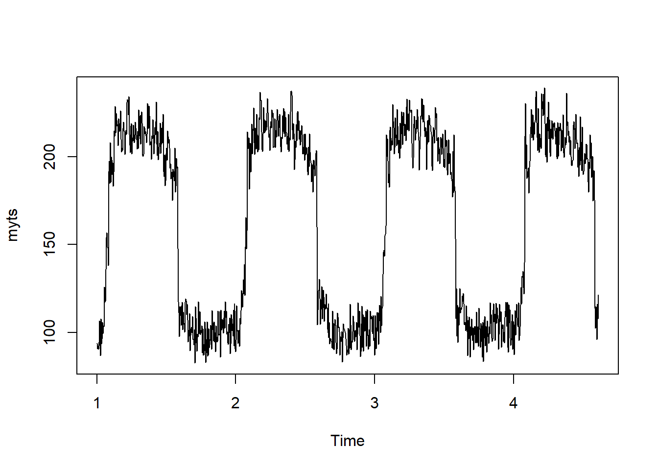
Looking at the data we see that the relationship between appliances and watt is unidirectional as the number of appliances impact the electricity consumption and not vice versa. Therefore, appliances can be used as an external regressor in the model. Moreover, since electricity consumption fluctuates a lot daily, we will use daily frequency. Most models are not good at handling large frequency data. One way out of this problem is to use the aggregation. But this might lead to over smoothening in the data. We also check for all the columns to have same length and all of them being numeric. There are many packages that allows one to compute neural net models. However, \(nnetar()\) from forecast is most user friendly. One handy thing about \(nnetar()\) is automatic selection of parameters. For more advanced implementation of the neural nets one can look at \(mlp()\) function form nnfor package.
## Warning: Missing column names filled in: 'X1' [1]## Parsed with column specification:
## cols(
## X1 = col_double(),
## watt = col_double(),
## appliances = col_double()
## )
theme_set(theme_bw())
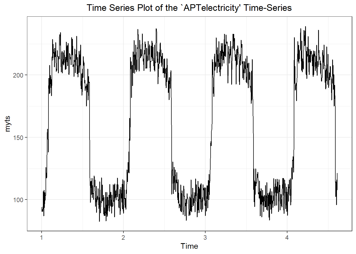
autoplot(myts) + ggtitle("Time Series Plot of the `APTelectricity' Time-Series") +
    theme(plot.title = element_text(hjust = 0.5))
set.seed(34)
# nnetar() requires a numeric vector or time series object as
# input ?nnetar() can be seen for more info on the function
# nnetar() by default fits multiple neural net models and
# gives averaged results xreg option allows for only numeric
# vectors in nnetar() function
fit = nnetar(myts)
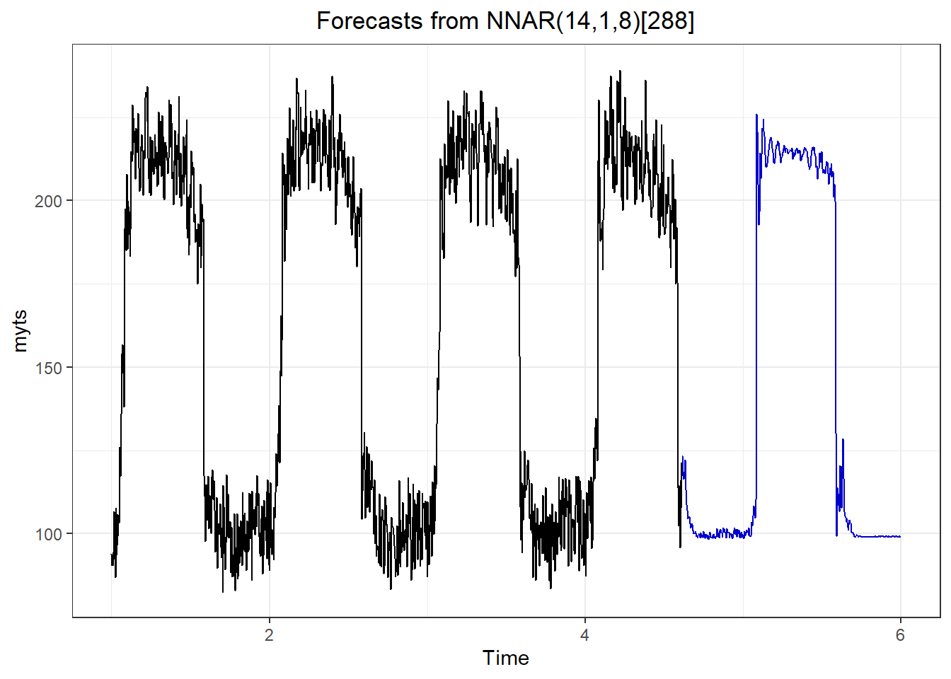
nnetforecast <- forecast(fit, h = 400, PI = F)  #Prediction intervals do not come by default in neural net forecasts, in constrast to ARIMA or exponential smoothing model
autoplot(nnetforecast) + theme(plot.title = element_text(hjust = 0.5))
For forecast of neural net models with external regressor, we need to have future values of the external regressor to be fed in the forecast function. More than one external regressors can be used in the forecast of the neural net models.
# Defining the vector which we want to forecast
y = rep(2, times = 12 * 10)
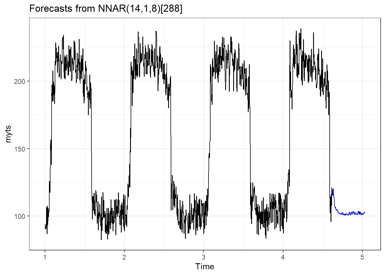
nnetforecast <- forecast(fit2, xreg = y, PI = F)
autoplot(nnetforecast)