Introduction to Time Series Analysis and Forecasting in R
2019-08-19
Chapter 1 Introduction
# on publishing the website see this
# https://bookdown.org/__docs__/user/publishing.html#publishing
rm(list = ls())
setwd("C:/Users/Tejendra/Desktop/FoldersOnDesktop/UdemyCourse/Section1")
require(tidyverse)
require(tidymodels)
require(data.table)
require(tidyposterior)
require(tsibble)  #tsibble for time series based on tidy principles
require(fable)  #for forecasting based on tidy principles
require(ggfortify)  #for plotting timeseries
require(forecast)  #for forecast function
require(tseries)
require(chron)
require(lubridate)
require(directlabels)
require(zoo)
# loading the data
ts1 <- read_delim("ITstore-bidaily.csv", ";", escape_double = FALSE,
col_names = FALSE, trim_ws = TRUE)## Parsed with column specification:
## cols(
## X1 = col_double(),
## X2 = col_double()
## )# declaring the data as time series
ts1 <- ts(ts1$X2, start = 1, frequency = 12, class = "ts")
# visualizing the time series
theme_set(theme_minimal())
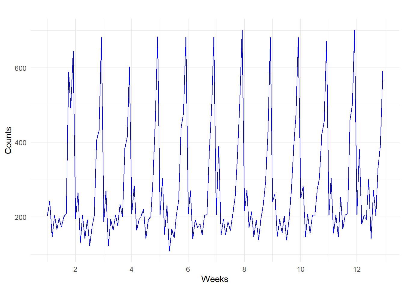
autoplot(ts1, color = "blue") + xlab("Weeks") + ylab("Counts")

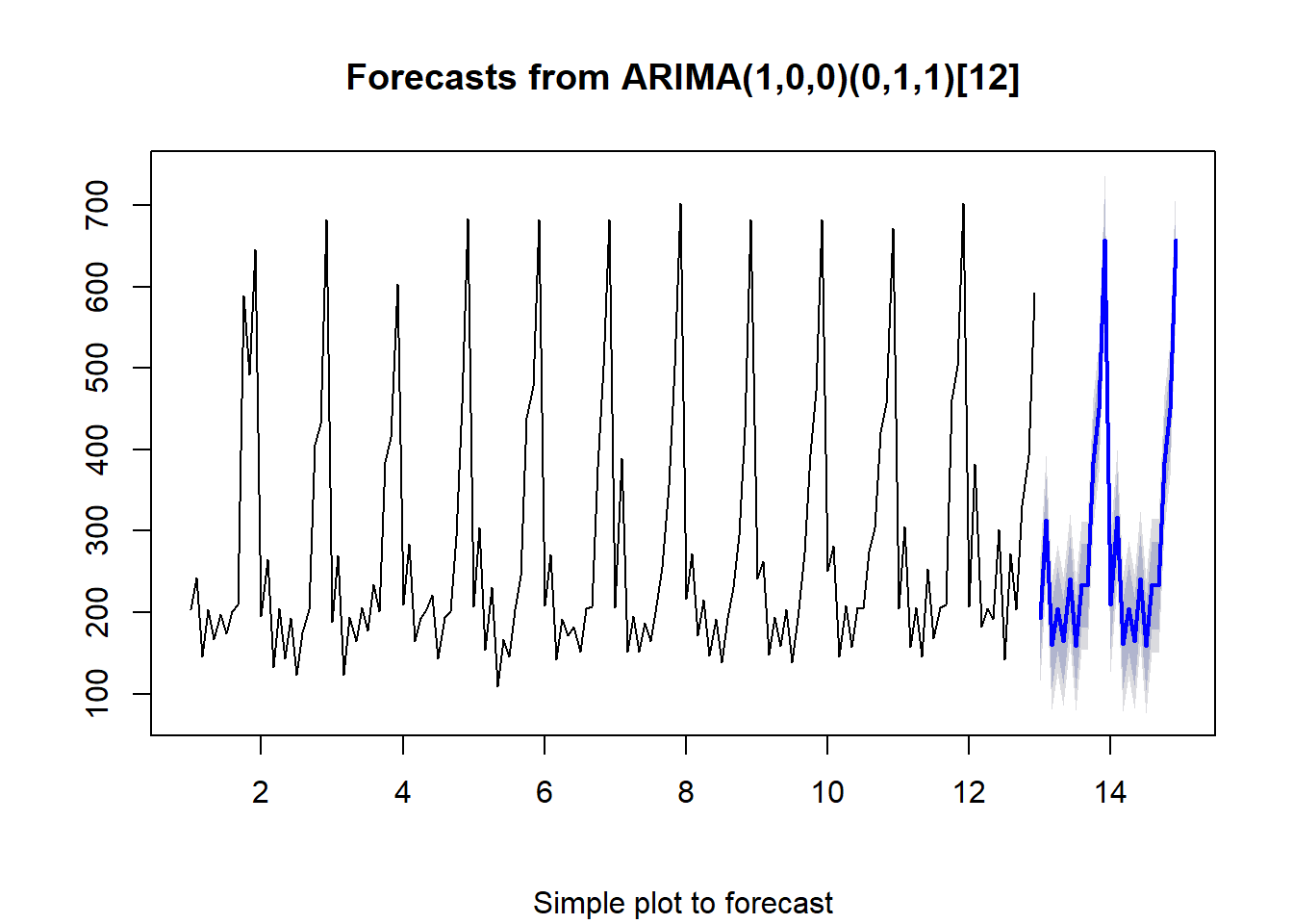
 Selecting the model.
Due to seasonality involved, simple models will not be able to capture it. We therefore use the seasonal ARIMA and exponential smoothing models. Exponential smoothing models have seasonality built in it by construction. Complex models like mixed models and neural nets will be an overkill.
