Chapter 2 Introduction
The R Statistical Software, developed and maintained by the R Core Team, may be considered as a powerful tool for the statistical community. The software being a Free Open Source Software is simply icing on the cake. R is evolving as the preferred companion of the Statistician. The reasons are aplenty. To begin with, this software has been developed by a team of Statisticians. Ross Ihaka and Robert Gentleman laid the basic framework for R, and later a group was formed who are responsible for the current growth and state of it. R is a command-line software and thus powerful with a lot of options for the user.
2.1 R Installation
The website http://cran.r-project.org/ consists of all versions of R available for a variety of
Operating Systems. CRAN is an abbreviation for Comprehensive R Archive Network. An incidental fact is that R had been developed on the Internet only. A user of Windows first needs to download the recent versions executable file, currently R-4.1.2-win.exe, and then merely double-click to complete the installation process.
A better way of becoming familiar with a software is to start with simple and useful programs. In this chapter, we aim to make the reader feel at home with the R software. The reader often struggles with the syntax of a software, and it is essentially this shortcoming that the reader will overcome after going through the later sections.
2.2 Familiarization of environments in R
Consider for a moment how your computer stores files. Every file is saved in a folder, and each folder is saved in another folder, which forms a hierarchical file system. If your computer wants to open up a file, it must first look up the file in this file system.
You can see your file system by opening a finder window. For example, Figure 2.1 shows part of the file system on my computer. I have hundreds of folders. Inside one of them is a subfolder named Documents, inside of that subfolder is a sub-subfolder named ggsubplot, inside of that folder is a folder named inst, inside of that is a folder named doc, and inside of that is a file named manual.pdf.
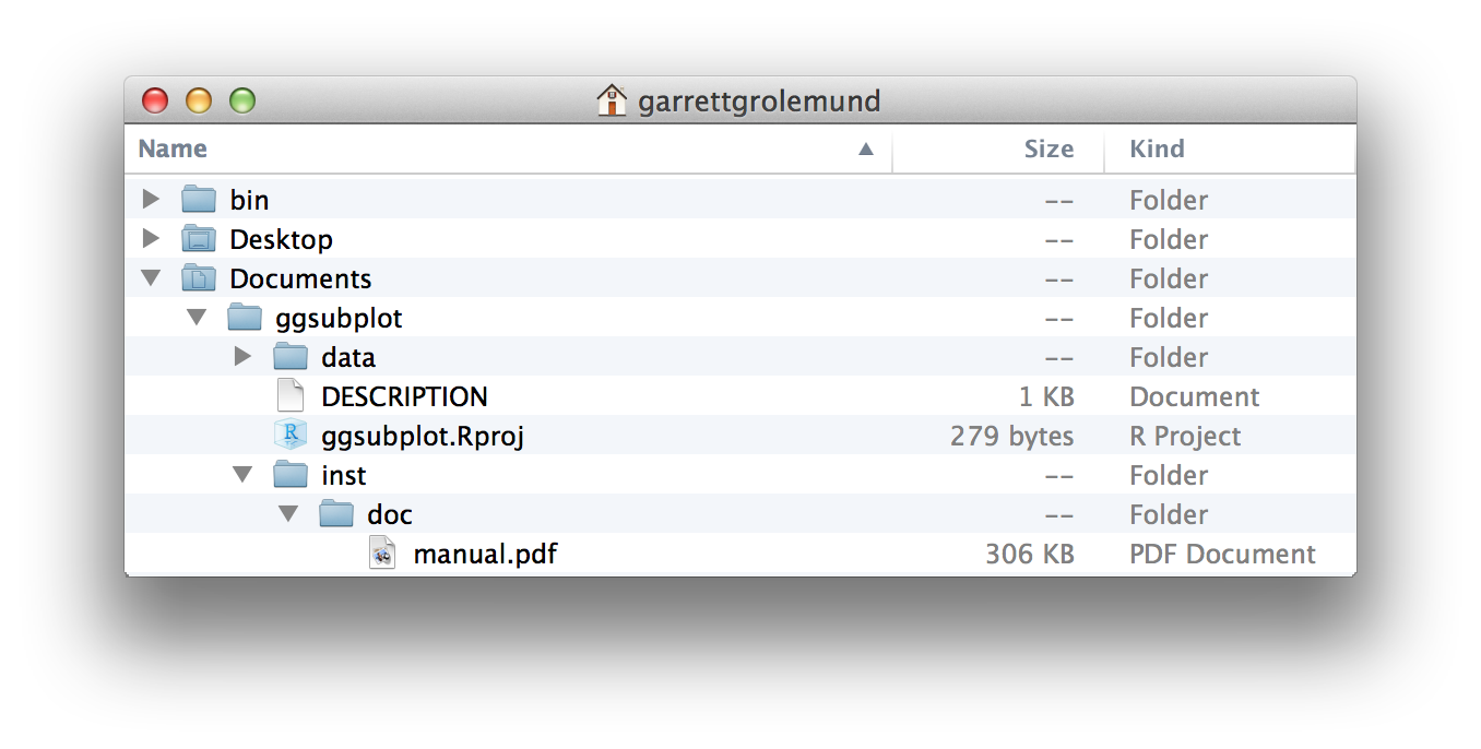
Figure 2.1: Your computer arranges files into a hierarchy of folders and subfolders. To look at a file, you need to find where it is saved in the file system.
R uses a similar system to save R objects. Each object is saved inside of an environment, a list-like object that resembles a folder on your computer. Each environment is connected to a parent environment, a higher-level environment, which creates a hierarchy of environments.
You can see R’s environment system with the parenvs function in the pryr package (note parenvs came in the pryr package when this book was first published). parenvs(all = TRUE) will return a list of the environments that your R session is using. The actual output will vary from session to session depending on which packages you have loaded.
R’s environments exist in your RAM memory, and not in your file system. Also, R environments aren’t technically saved inside one another. Each environment is connected to a parent environment, which makes it easy to search up R’s environment tree. But this connection is one-way: there’s no way to look at one environment and tell what its “children” are. So you cannot search down R’s environment tree. In other ways, though, R’s environment system works similar to a file system. R works closely with the environment tree to look up objects, store objects, and evaluate functions. How R does each of these tasks will depend on the current active environment.
2.2.1 The Active Environment
At any moment of time, R is working closely with a single environment. R will store new objects in this environment (if you create any), and R will use this environment as a starting point to look up existing objects (if you call any). I’ll call this special environment the active environment. The active environment is usually the global environment, but this may change when you run a function.
You can use environment to see the current active environment:
environment()## <environment: R_GlobalEnv>The global environment plays a special role in R. It is the active environment for every command that you run at the command line. As a result, any object that you create at the command line will be saved in the global environment. You can think of the global environment as your user workspace.
When you call an object at the command line, R will look for it first in the global environment. But what if the object is not there? In that case, R will follow a series of rules to look up the object.
R saves its objects in an environment system that resembles your computer’s file system. If you understand this system, you can predict how R will look up objects. If you call an object at the command line, R will look for the object in the global environment and then the parents of the global environment, working its way up the environment tree one environment at a time.
R will use a slightly different search path when you call an object from inside of a function. When you run a function, R creates a new environment to execute commands in. This environment will be a child of the environment where the function was originally defined. This may be the global environment, but it also may not be. You can use this behavior to create closures, which are functions linked to objects in protected environments.
As you become familiar with R’s environment system, you can use it to produce elegant results, like we did here. However, the real value of understanding the environment system comes from knowing how R functions do their job. You can use this knowledge to figure out what is going wrong when a function does not perform as expected.
2.3 Basic math and stat using R
This section is devoted to transform your math or stat knowledge in computational form. R will serve you as a scientific calculator with programming functionality.
2.3.1 Perform simple arithmetics using R.
In this section (section 2.3.1) we will focus on the functionality of R as a calculator. We will begin with simple addition, multiplication, and power computations. The codes/programs in R are read from left to right, and executed in that order.
57 + 89## [1] 14645 - 87 # find difference## [1] -4260 * 3 # find product## [1] 1807/18 # find quotient ## [1] 0.38888894^4 # calculating power## [1] 256It is implicitly assumed (and implemented too) that any reliable computing software must have included the brackets, orders, division, multiplication, addition, and subtraction, BODMAS rule. It means that if the user executes \(4 \times 3^3\), the answer is 108, that is, order is first executed and then multiplication, and not 1728, multiplication followed by order. We verify the same next.
4*3^3## [1] 1082.3.2 Perform basic R functions.
In this section we will discuss R functions related to basic math and stat.
The absolute value of elements or vectors can be found using the abs command. For example:
l1=-4:3 # creating a sequence of numbers from -4 to 3 with step size 1
l1
## [1] -4 -3 -2 -1 0 1 2 3abs(l1) # returns absolute value of l1## [1] 4 3 2 1 0 1 2 3Remainders can be computed using the R operator %%.
(-4:3) %% 3## [1] 2 0 1 2 0 1 2 0The integer divisor between two numbers may be calculated using the %/% operation.
(-4:4) %/% 3## [1] -2 -1 -1 -1 0 0 0 1 1The sign operator tells whether an element is positive, negative, or neither.
sign(-4:3)## [1] -1 -1 -1 -1 0 1 1 1The number of digits to which R gives answers is set at seven digits by default. There are multiple ways to obtain our answers in the number of digits that we actually need. For instance, if we require only two digits accuracy for 7/18, we can use the following:
round(7/18,2)## [1] 0.39It is often of interest to obtain the greatest integer less than the given number, or the least integer greater than the given number. Such tasks can be handled by the functions
floorandceilingrespectively. For instance:
floor(3.1415)## [1] 3ceiling(0.618)## [1] 1Sum of values store in variables can be found using the sum function in R.
a=5;b=10
paste0("sum is:", sum(a,b))
## [1] "sum is:15"Note: An array in R usually created with the combine (syntax :
c(variables)) function.
val=c(1,2,6,7,8,3,5,7)
sum(val)
## [1] 39Other similar math functions are: all, any, prod, min, max, and range. The last five of these is straightforward for the user to apply to their problems. This is illustrated by the following.
prod(val)## [1] 70560min(val)## [1] 1max(val)## [1] 8range(val)## [1] 1 8Now we are left to understand the R functions any and all. The any function checks if it is true that the array under consideration meets certain criteria. As an example, suppose we need to know if there are some elements of \((-1,3,4,-9,4)\) less than 0.
any(c(-1,3,4,-9,4)<0)## [1] TRUEall(c(1,6,-14,-154,0)<0) # all checks if criteria is met by each element## [1] FALSETrigonometric functions are very useful tools in statistical analysis of data. It is worth mentioning the emerging areas where this is frequently used. Wavelet analysis, functional data analysis, and time series spectral analysis are a few examples. Such a discussion is however beyond the scope of this current book.We will contain ourself with a very elementary session. The value of 𝜋 is stored as one of the constants in R.
sin(pi/2)## [1] 1atan(0) # atan calculate inverse tan## [1] 0log(exp(1)) # log calculate natural logarithm## [1] 1Arc-cosine, arc-sine, and arc-tangent functions are respectively obtained using acos, asin, and atan. Also, the hyperbolic trigonometric functions are available in cosh, sinh, tanh, acosh, asinh, and atanh.
2.3.3 Complex numbers in R
Complex numbers can be handled easily in R. Its use is straightforward and the details are obtained by keying in ?complex or ?Complex at the terminal. As the arithmetic related to complex numbers is a simple task, we will look at an interesting case where the functions of complex numbers arise naturally. To input a complex number \(1+i\), write c=1+1i.
1+1i## [1] 1+1iexp(1i*pi)## [1] -1+0iNote that \(e^{i\pi}=\cos \pi+i\sin \pi=-1+i 0\).
For the illustration purpose, the characteristic function of a uniform distribution in \([-1,1]\) (\(\varphi(t)=\dfrac{e^{itb}-e^{ita}}{it(b-a)}\)) can be simulated in R as follows:
# Plot of Characteristic Function of a U(-1,1) Random Variable
a <- -1; b <- 1
t <- seq(-20,20,.1)
chu <- (exp(1i*t*b)-exp(1i*t*a))/(1i*t*(b-a))
plot(t,chu,"l",ylab=(expression(varphi(t))),main="Characteristic  Function of Uniform Distribution [-1, 1]")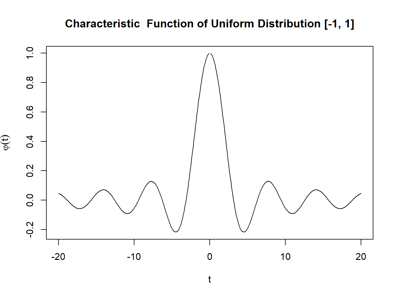
Figure 2.2: Characteristic function of Uniform Distribution
2.3.4 Special Mathematical Functions
Here, by special functions, we mean certain mathematical entities that are difficult to calculate as the series/range increases. Factorials do have an in-built function in factorial. A few examples are in order.
Factorial
factorial(3)## [1] 6Combination
Consider the classical problem of selecting r-out-of-n objects. If we have to select k objects with replacement, that is the first drawn object is replaced in the pack before the second object is drawn, the number of ways of accomplishing the task is \(\binom n k\). If n = 10 and r = 4, the
choose function gives us the desired answer through the arguments n and k. That is, \(\binom n k\) is calculated in R with choose(n,k).
n=10;k=4
choose(n,k)
## [1] 210Permutation
The permutation operation is defined as \(^n P_r=n\times (n-1)\times \cdots \times (n-r+1)\). So we can use prod function in R to find \(^{10}P_4\) as:
prod(10:(10-4+1)) # permutations of 10 p 4## [1] 5040All the functions used in this chapter are taken from the R base library (R Core Team 2021).