20IMCAL204 STATISTICS LAB- Laboratory Manual
2022-04-06
Chapter 1 Preface
This course is designed as a Computational Statistics Laboratory (CSL) comprised of 29 experiments selected from the Statistical Courses in INMCA Programme. Details of experiments and the instructions regarding creation & submission of laboratory reports are explained in this introductory chapter.
1.1 Details of Experiments
Familiarization of environments in R.
Perform simple arithmetics using R.
Perform basic R functions.
Use various graphical techniques in EDA.
Create different charts for visualization of given set of data.
Draw a Pareto chart to illustrate the Pareto principle.
Find the mean, median, standard deviation and quartiles of a set of observations.
Find the Skewness and Kurtosis of a given dataset distribution.
Given the scenario, implement the Bayes rule by finding the posterior probability.
Find the mass function of a binomial distribution with \(n=20,\, p=0.4\). Also draw the graphs of the mass function and cumulative distribution function.
Given the data n=50, mean=25, use appropriate function to find the mass function of a Poisson distribution. Also draw the graphs of the mass function and cumulative distribution function.
Use appropriate function to generate the pdf of the exponential distribution with mean 30 , take x values 0 to 1 with 0.25 difference. Draw the graph of the density function.
Generate and draw the cdf and pdf of a normal distribution with mean=10 and standard deviation=3. Use values of \(x\) from 0 to 20 in intervals of 1.
The following data shows the result of throwing 12 fair dice 4,096 times; a throw of 4,5, or 6 being called success.
\(\begin{array}{|l|cccccccccccc|}\hline \text{Success(X)}:& 0 &1& 2& 3& 4 &5& 6& 7& 8& 9& 10& 11& 12\\\hline \text{Frequency(f)}:& 0 &7& 60& 198& 430& 731& 948& 847& 536& 257& 71& 11& 0\\\hline \end{array}\)
Fit a binomial distribution and find the expected frequencies. Compare the graphs of the observed frequency and theoretical frequency.
- From the following data, compute Karl Pearson’s coefficient of correlation. (Using actual mean method).
\(\begin{array}{|l|ccccccc|}\hline \text{Price(Rupees)}:& 10& 20& 30& 40& 50& 60& 70\\\hline \text{Supply(Units)}:& 8& 6& 14& 16& 10& 20& 24\\\hline \end{array}\)
- From the following data compute correlation between height of father and height of daughters by Karl Pearson’s coefficient of correlation.
\(\begin{array}{|l|cccccccc|}\hline \text{Height of Father(Cms)}& 65& 66& 67& 67& 68& 69& 71& 73\\\hline \text{Height of Daughter(Cms)}& 67& 68& 64& 69& 72& 70& 69& 73\\\hline \end{array}\)
- The scores for nine students in history and algebra are as follows:
\(\begin{array}{|l|ccccccccc|}\hline \text{History}:&35& 23& 47& 17& 10& 43& 9& 6&28\\\hline \text{Algebra}:&30& 33&45&23&8&49&12&4&31\\\hline \end{array}\)
Compute the Spearman rank correlation.
Calculate the regression coefficient and obtain the lines of regression for the given data.
Construct a scatter plot to investigate the relationship between two variables.
Compute confidence intervals for the mean when the standard deviation is known.
Perform the Z- test for single proportion.
Perform the Z-test for difference in proportion.
Perform the Z- test for single mean.
Perform the Z- test for difference in mean.
Perform t-test for mean.
Perform t test for equality of mean.
Perform Paired t test.
Perform F test
Perform Chi-Square test.
1.2 Preparation of Lab report
Since R Studio supports markdown documentation facility, the students are advised to create the Lab report in the form of a Rmarkdown file. Each experiment should have the Experiment no and the title. The first section of each experiment is Aim, then write the Algorithm, then Code and finally the output of the program. A sample lab session report is given below:
1.3 Experiment No: 17- Spearman Rank Correlation
1.3.1 Aim:
Find the Spearman rank correlation of two variables given in the form of table using R programming.
1.3.2 Algorithm
- Step 1: Read the data into R
- Step 2: write the function syntax to calculate Spearman rank correlation
- Step 3: Apply the function on the set of data
- Step 4: Report the correlation coefficient
- Step 5: Interpretation based on the coefficient
1.3.3 R code
height_F=c(65,66,67,67,68,69,71,73)
height_D=c(67,68,64,69,72,70,69,73)
resp2=cor.test(height_F,height_D,method='spearman')
## Warning in cor.test.default(height_F, height_D, method = "spearman"): Cannot
## compute exact p-value with tiesresp2##
## Spearman's rank correlation rho
##
## data: height_F and height_D
## S = 19.735, p-value = 0.02698
## alternative hypothesis: true rho is not equal to 0
## sample estimates:
## rho
## 0.76506021.3.4 Result & Interpretations
The spearman correlation between the given set of data is 0.7650602.
Interpretation: Here the Spearman rank coefficient is 0.7650602. Also p-value is 0.0269756 <0.05. So the null hypothesis is rejected. So it is statistically reasonable to conclude that there is significant positive correlation between the price and supply based on the sample.
We can show the correlation in the form of scatter plot as follows:
library("ggpubr")## Loading required package: ggplot2data1=data.frame(height_F,height_D)
ggscatter(data1, x = "height_F", y = "height_D",
add = "reg.line", conf.int = TRUE,
cor.coef = TRUE, cor.method = "pearson",
xlab = "Height of Father (cm)", ylab = "Height of Daughter (cm)")## `geom_smooth()` using formula 'y ~ x'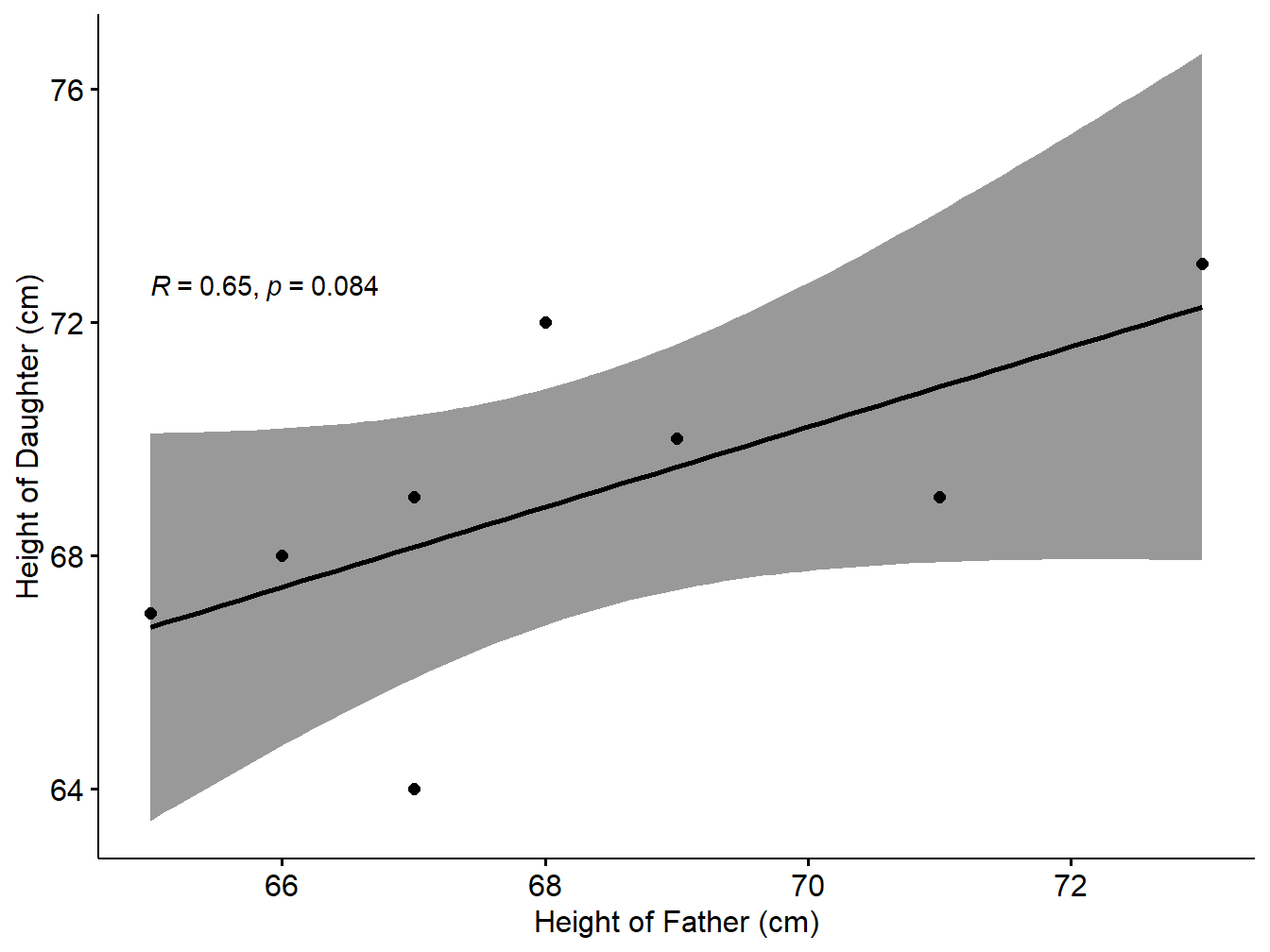
Figure 1.1: Scatter plot with smooth fit curve
1.4 Computational Source
This manual is prepared based on the books (Navarro 2013) and (Prabhanjan and Tattar 2016).