Chapter 6 Inferential Statistics & Testing of Hypothesis
6.1 Study of Confidence Intervals for Means of Large and Small Samples
6.1.1 Calculate confidence interval in R – Normal distribution
Given the parameters of the population proportion distribution and sample standard deviation, generate the bootstrap confidence interval. In this situation, we’re basically using r like an error interval calculator… Using the 95 percent confidence level and confidence coefficient function, we will now create the R code for a confidence interval. What does a 95 percent confidence interval mean? Essentially, a calculating a 95 percent confidence interval in R means that we are 95 percent sure that the true probability falls within the confidence interval range that we create in a standard normal distribution.
\[CI=\bar{X}\pm t_{0.975}SE\]
# Calculate Confidence Interval in R for Normal Distribution
# Confidence Interval Statistics
# Assume mean of 12
# Standard deviation of 3
# Sample size of 30
# 95 percent confidence interval so right tail at 0.975
xbar <- 12
stddev <- 3
n <- 30
error <- qnorm(0.975)*stddev/sqrt(n)
lower_bound <- xbar - error
upper_bound <- xbar + error
lower_bound
## [1] 10.92648upper_bound## [1] 13.073526.1.2 Calculate Confidence Interval in R – t distribution
For experiments run with small sample sizes it is generally inappropriate to use the standard normal distribution or normal approximation. For more accurate small sample hypothesis testing a student T distribution is the correct choice for this environment. A t confidence interval is slightly different from a normal or percentile approximate confidence interval in R. When creating a approximate confidence interval using a t table or student t distribution, you help to eliminate some of the variability in your data by using a slightly different base dataset binomial distribution.
R can support this by substituting the qt function for the qnorm function, as demonstrated below…. assume we are working with a semi large sample size of 15. You will need to tell the qt function the degrees of freedom as a parameter (should be n-1).
# Calculate Confidence Interval in R for t Distribution
# t test confidence interval
# Assume mean of 12
# Standard deviation of 3
# Sample size of 15
# 95% confidence interval so the right tail at .975
xbar <- 12
stddev <- 3
n <- 30
error <- qt(0.975,df=n-1)*stddev/sqrt(n)
lower_bound <- xbar - error
upper_bound <- xbar + error
lower_bound
## [1] 10.87978upper_bound## [1] 13.120226.2 Large Sample Tests
6.2.1 One-Proportion Z-Test in R
The One proportion Z-test is used to compare an observed proportion to a theoretical one, when there are only two categories.
For example, we have a population of mice containing half male and have female (p = 0.5 = 50%). Some of these mice (n = 160) have developed a spontaneous cancer, including 95 male and 65 female.We want to know, whether the cancer affects more male than female?
Typical research questions are:
- whether the observed proportion of male (po) is equal to the expected proportion (pe)?
- whether the observed proportion of male (po) is less than the expected proportion (pe)?
- whether the observed proportion of male (p) is greater than the expected proportion (pe)?
In statistics, we can define the corresponding null hypothesis (\(H_0\)) as follow:
- \(H_0:p_o=p_e\)
- \(H_0:p_o≤p_e\)
- \(H_0:p_o≥p_e\)
The corresponding alternative hypotheses (\(H_a\)) are as follow:
- \(H_a:p_o≠p_e\) (different, two tailed)
- \(H_a:p_o>p_e\) (greater,right tailed)
- \(H_a:p_o<p_e\) (less, left tailed)
The test statistic (also known as z-test) can be calculated as follow:
\[z = \frac{p_o-p_e}{\sqrt{p_oq/n}}\] The confidence interval of \(p_o\) at 95% is defined as follow: \[p_o \pm 1.96\sqrt{\frac{p_oq}{n}}\]
6.2.2 Compute one proportion z-test in R
The R functions binom.test() and prop.test() can be used to perform one-proportion test:
Syntax:
prop.test(x, n, p = NULL, alternative = "two.sided",correct = TRUE)
- x: the number of of successes
- n: the total number of trials
- p: the probability to test against.
- correct: a logical indicating whether Yates’ continuity correction should be applied where possible.
Now let’s test our hypothesis that whether the cancer affects more male than female? using R
resprop=prop.test(x = 95, n = 160, p = 0.5, correct = FALSE,
           alternative = "greater")
resprop
##
## 1-sample proportions test without continuity correction
##
## data: 95 out of 160, null probability 0.5
## X-squared = 5.625, df = 1, p-value = 0.008853
## alternative hypothesis: true p is greater than 0.5
## 95 percent confidence interval:
## 0.5288397 1.0000000
## sample estimates:
## p
## 0.59375Interpretation: The p-value of the test is 0.008853, which is less than the significance level alpha = 0.05. So the null hypothesis is rejected. We can conclude that the proportion of male with cancer is not significantly high with a p-value = 0.008853.
Confidance interval for proportion: A 95% confidance interval for observed proportion can be found using following code:
# printing the confidence interval
resprop$conf.int
## [1] 0.5288397 1.0000000
## attr(,"conf.level")
## [1] 0.956.2.3 Two sample Z-test
The two-proportions z-test is used to compare two observed proportions. For example, we have two groups of individuals: * Group A with lung cancer: \(n = 500\) * Group B, healthy individuals: \(n = 500\)
The number of smokers in each group is as follow:
- Group A with lung cancer: \(n = 500\), 490 smokers, \(p_A=490/500=0.98\)
- Group B, healthy individuals: \(n = 500\), 400 smokers, \(p_B=400/500=0.80\)
In this setting:
- The overall proportion of smokers is \(p=\frac{(490+400)}{500+500}=0.89\)
- The overall proportion of non-smokers is \(q=1−p=0.11\)
We want to know, whether the proportions of smokers are the same in the two groups of individuals?
The research questions related to this senario are:
Questions! 1. whether the observed proportion of smokers in group A (\(p_A\)) is equal to the observed proportion of smokers in group (\(p_B\))?
whether the observed proportion of smokers in group A (\(p_A\)) is less than the observed proportion of smokers in group (\(p_B\))?
whether the observed proportion of smokers in group A (\(p_A\)) is greater than the observed proportion of smokers in group (\(p_B\))?
In statistics, we can define the corresponding null hypothesis (\(H_0\)) as follow:
- \(H_0:p_A=p_B\)
- \(H_0:p_A≤p_B\)
- \(H_0:p_A≥p_B\)
The corresponding alternative hypotheses (\(H_a\)) are as follow:
- \(H_a:p_A≠p_B\) (different)
- \(H_a:p_A>p_B\) (greater)
- \(H_a:p_A<p_B\) (less)
6.2.3.1 Conducting two-sample proportion Z-test
restsp <- prop.test(x = c(490, 400), n = c(500, 500))
# Printing the results
restsp
##
## 2-sample test for equality of proportions with continuity correction
##
## data: c(490, 400) out of c(500, 500)
## X-squared = 80.909, df = 1, p-value < 2.2e-16
## alternative hypothesis: two.sided
## 95 percent confidence interval:
## 0.1408536 0.2191464
## sample estimates:
## prop 1 prop 2
## 0.98 0.80Interpretation of the result: The p-value of the test is \(2.2^{-16}\), which is less than the significance level alpha = 0.05. We can conclude that the proportion of smokers is significantly different in the two groups with a p-value = \(2.2^{-16}\).
6.2.4 Compare means of Large Samples (z-test)
You can use the z.test() function from the BSDA package to perform one sample and two sample z-tests in R.
This function uses the following basic syntax:
> Syntax: z.test(x, y, alternative='two.sided', mu=0, sigma.x=NULL, sigma.y=NULL,conf.level=.95)
where:
- x: values for the first sample
- y: values for the second sample (if performing a two sample z-test) *alternative: the alternative hypothesis (‘greater,’ ‘less,’ ‘two.sided’)
- mu: mean under the null or mean difference (in two sample case)
- sigma.x: population standard deviation of first sample
- sigma.y: population standard deviation of second sample
- conf.level: confidence level to use
Example: Suppose the IQ in a certain population is normally distributed with a mean of \(\mu\) = 100 and standard deviation of \(\sigma\) = 15. A scientist wants to know if a new medication affects IQ levels, so she recruits 20 patients to use it for one month and records their IQ levels at the end of the month.
Solution: The following code shows how to perform a one sample z-test in R to determine if the new medication causes a significant difference in IQ levels: Here the null hypothesis is that the medication has no effect (ie., \(\mu_0=\mu=100\))
The following examples shows how to use this function in practice.
library(BSDA)## Loading required package: lattice##
## Attaching package: 'BSDA'## The following object is masked from 'package:datasets':
##
## Orange#enter IQ levels for 20 patients
data = c(88, 92, 94, 94, 96, 97, 97, 97, 99, 99,
105, 109, 109, 109, 110, 112, 112, 113, 114, 115)
#perform one sample z-test
z.test(data, mu=100, sigma.x=15,alternative="two.sided")##
## One-sample z-Test
##
## data: data
## z = 0.90933, p-value = 0.3632
## alternative hypothesis: true mean is not equal to 100
## 95 percent confidence interval:
## 96.47608 109.62392
## sample estimates:
## mean of x
## 103.05The test statistic for the one sample z-test is 0.90933 and the corresponding p-value is 0.3632.
Since this p-value is not less than .05, we do not have sufficient evidence to reject the null hypothesis. Thus, we conclude that the new medication does not significantly affect IQ level.
6.2.5 Two Sample Z-Test in R
Suppose the IQ levels among individuals in two different cities are known to be normally distributed each with population standard deviations of 15.
A scientist wants to know if the mean IQ level between individuals in city A and city B are different, so she selects a simple random sample of 20 individuals from each city and records their IQ levels.
The following code shows how to perform a two sample z-test in R to determine if the mean IQ level is different between the two cities:
#enter IQ levels for 20 individuals from each city
cityA = c(82, 84, 85, 89, 91, 91, 92, 94, 99, 99,
         105, 109, 109, 109, 110, 112, 112, 113, 114, 114)

cityB = c(90, 91, 91, 91, 95, 95, 99, 99, 108, 109,
         109, 114, 115, 116, 117, 117, 128, 129, 130, 133)

#perform two sample z-test
z.test(x=cityA, y=cityB, mu=0, sigma.x=15, sigma.y=15)
##
## Two-sample z-Test
##
## data: cityA and cityB
## z = -1.7182, p-value = 0.08577
## alternative hypothesis: true difference in means is not equal to 0
## 95 percent confidence interval:
## -17.446925 1.146925
## sample estimates:
## mean of x mean of y
## 100.65 108.80The test statistic for the two sample z-test is -1.7182 and the corresponding p-value is 0.08577. Since this p-value is not less than .05, we do not have sufficient evidence to reject the null hypothesis. Thus, we conclude that the mean IQ level is not significantly different between the two cities.
6.3 Small Sample Tests
6.3.1 One sample t-test
To perform one-sample t-test, the R function t.test() can be used as follow:
Syntax: `t.test(x, mu = 0, alternative = c(“greater,”“less,”“two.sided”)’
Lets create the following synthetic data of 20 mice to test whter the average weight of the mice population is 25g or not.
We want to know, if the average weight of the mice differs from 25g?
set.seed(1234)
my_data <- data.frame(
  name = paste0(rep("M_", 10), 1:10),
  weight = round(rnorm(10, 20, 2), 1)
)
Check the data:
# Print the first 10 rows of the data
head(my_data, 10)
## name weight
## 1 M_1 17.6
## 2 M_2 20.6
## 3 M_3 22.2
## 4 M_4 15.3
## 5 M_5 20.9
## 6 M_6 21.0
## 7 M_7 18.9
## 8 M_8 18.9
## 9 M_9 18.9
## 10 M_10 18.2# Statistical summaries of weight
summary(my_data$weight)## Min. 1st Qu. Median Mean 3rd Qu. Max.
## 15.30 18.38 18.90 19.25 20.82 22.20#priliminary check for normality
shapiro.test(my_data$weight) # => p-value = 0.6993, so null hypothesis is accepted##
## Shapiro-Wilk normality test
##
## data: my_data$weight
## W = 0.9526, p-value = 0.6993Now perform the one sample t-test:
# One-sample t-test
rest1 <- t.test(my_data$weight, mu = 25)
# Printing the results
rest1
##
## One Sample t-test
##
## data: my_data$weight
## t = -9.0783, df = 9, p-value = 7.953e-06
## alternative hypothesis: true mean is not equal to 25
## 95 percent confidence interval:
## 17.8172 20.6828
## sample estimates:
## mean of x
## 19.25The p-value of the test is 7.9533835^{-6} , which is less than the significance level alpha = 0.05. We can conclude that the mean weight of the mice is significantly different from 25g with a p-value = 7.9533835^{-6}.
6.3.2 Two-sample t-test
Welch’s t-test is used to compare the means between two independent groups when it is not assumed that the two groups have equal variances.
To perform Welch’s t-test in R, we can use the t.test() function, which uses the following syntax:
Syntax:
t.test(x, y, alternative = c(“two.sided”, “less”, “greater”))
Example: A teacher wants to compare the exam scores of 12 students who used an exam prep booklet to prepare for some exam vs. 12 students who did not. The following vectors show the exam scores for the students in each group:
booklet <- c(90, 85, 88, 89, 94, 91, 79, 83, 87, 88, 91, 90)
no_booklet <- c(67, 90, 71, 95, 88, 83, 72, 66, 75, 86, 93, 84)
SOlution: Before we perform a Welch’s t-test, we can first create boxplots to visualize the distribution of scores for each group:
boxplot(booklet, no_booklet, names=c("Booklet","No Booklet"))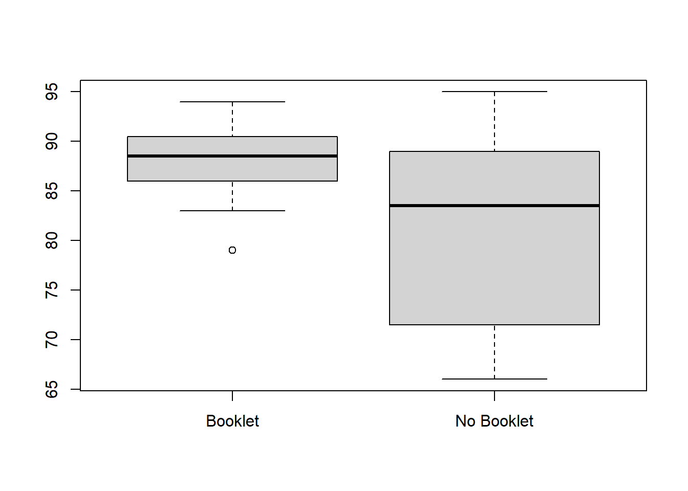 We can clearly see that the “Booklet” group has a higher mean score and lower variance in scores.
To formally test whether or not the mean scores between the groups are significantly different, we can perform Welch’s t-test:
#perform Welch's t-test
t.test(booklet, no_booklet,alternative = "two.sided")
##
## Welch Two Sample t-test
##
## data: booklet and no_booklet
## t = 2.2361, df = 14.354, p-value = 0.04171
## alternative hypothesis: true difference in means is not equal to 0
## 95 percent confidence interval:
## 0.3048395 13.8618272
## sample estimates:
## mean of x mean of y
## 87.91667 80.83333From the output we can see that the t test-statistic is 2.2361 and the corresponding p-value is 0.04171.
Since this p-value is less than .05, we can reject the null hypothesis and conclude that there is a statistically significant difference in mean exam scores between the two groups.
6.3.3 Paired t-test
A paired samples t-test is a statistical test that compares the means of two samples when each observation in one sample can be paired with an observation in the other sample.
For example, suppose we want to know whether a certain study program significantly impacts student performance on a particular exam. To test this, we have 20 students in a class take a pre-test. Then, we have each of the students participate in the study program each day for two weeks. Then, the students retake a test of similar difficulty.
To compare the difference between the mean scores on the first and second test, we use a paired t-test because for each student their first test score can be paired with their second test score.
To conduct a paired t-test in R, we can use the built-in t.test() function with the following syntax:
Syntax:
t.test(x, y, paired = TRUE, alternative = “two.sided”)
The following example illustrates how to conduct a paired t-test to find out if there is a significant difference in the mean scores between a pre-test and a post-test for 20 students.
#create the dataset
data <- data.frame(score = c(85 ,85, 78, 78, 92, 94, 91, 85, 72, 97,
                             84, 95, 99, 80, 90, 88, 95, 90, 96, 89,
                             84, 88, 88, 90, 92, 93, 91, 85, 80, 93,
                             97, 100, 93, 91, 90, 87, 94, 83, 92, 95),
                   group = c(rep('pre', 20), rep('post', 20)))
#view the dataset
data
## score group
## 1 85 pre
## 2 85 pre
## 3 78 pre
## 4 78 pre
## 5 92 pre
## 6 94 pre
## 7 91 pre
## 8 85 pre
## 9 72 pre
## 10 97 pre
## 11 84 pre
## 12 95 pre
## 13 99 pre
## 14 80 pre
## 15 90 pre
## 16 88 pre
## 17 95 pre
## 18 90 pre
## 19 96 pre
## 20 89 pre
## 21 84 post
## 22 88 post
## 23 88 post
## 24 90 post
## 25 92 post
## 26 93 post
## 27 91 post
## 28 85 post
## 29 80 post
## 30 93 post
## 31 97 post
## 32 100 post
## 33 93 post
## 34 91 post
## 35 90 post
## 36 87 post
## 37 94 post
## 38 83 post
## 39 92 post
## 40 95 postA basic descriptive analysis can be carried out first:
#load dplyr library
library(dplyr)
##
## Attaching package: 'dplyr'## The following objects are masked from 'package:stats':
##
## filter, lag## The following objects are masked from 'package:base':
##
## intersect, setdiff, setequal, union#find sample size, mean, and standard deviation for each group
data %>%
group_by(group) %>%
summarise(
count = n(),
mean = mean(score),
sd = sd(score)
)## # A tibble: 2 x 4
## group count mean sd
## <chr> <int> <dbl> <dbl>
## 1 post 20 90.3 4.88
## 2 pre 20 88.2 7.24A box plot visualization is here:
boxplot(score~group,
data=data,
main="Test Scores by Group",
xlab="Group",
ylab="Score",
col="steelblue",
border="black"
)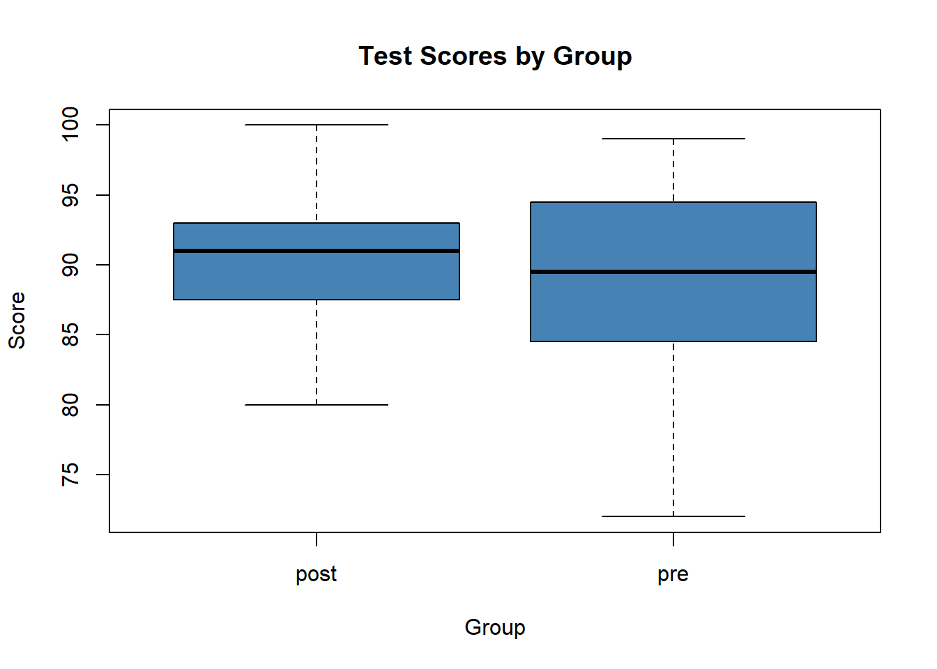 From both the summary statistics and the boxplots, we can see that the mean score in the post group is slightly higher than the mean score in the pre group. We can also see that the scores for the post group have less variability than the scores in the pre group.
To find out if the difference between the means for these two groups is statistically significant, we can proceed to conduct a paired t-test.
Before we conduct the paired t-test, we should check that the distribution of differences is normally (or approximately normally) distributed. To do so, we can create a new vector defined as the difference between the pre and post scores, and perform a shapiro-wilk test for normality on this vector of values:
#define new vector for difference between post and pre scores
differences <- with(data, score[group == "post"] - score[group == "pre"])

#perform shapiro-wilk test for normality on this vector of values
shapiro.test(differences)
##
## Shapiro-Wilk normality test
##
## data: differences
## W = 0.92307, p-value = 0.1135The p-value of the test is 0.1135, which is greater than alpha = 0.05. Thus, we fail to reject the null hypothesis that our data is normally distributed. This means we can now proceed to conduct the paired t-test.
We can use the following code to conduct a paired t-test:
t.test(score ~ group, data = data, paired = TRUE)##
## Paired t-test
##
## data: score by group
## t = 1.588, df = 19, p-value = 0.1288
## alternative hypothesis: true difference in means is not equal to 0
## 95 percent confidence interval:
## -0.6837307 4.9837307
## sample estimates:
## mean of the differences
## 2.15Thus, since our p-value is less than our significance level of 0.05 we will fail to reject the null hypothesis that the two groups have statistically significant means. In other words, we do not have sufficient evidence to say that the mean scores between the pre and post groups are statistically significantly different. This means the study program had no significant effect on test scores.
In addition, our 95% confidence interval says that we are “95% confident” that the true mean difference between the two groups is between -0.6837 and 4.9837. Since the value zero is contained in this confidence interval, this means that zero could in fact be the true difference between the mean scores, which is why we failed to reject the null hypothesis in this case.
6.4 F- Test
An F-test is used to test whether two population variances are equal. The null and alternative hypotheses for the test are as follows:
\(H_0: \sigma_1^2 = \sigma_2^2\) (the population variances are equal)
\(H_1: \sigma_1^2 \neq \sigma_2^2\) (the population variances are not equal)
To perform an F-test in R, we can use the function var.test() with one of the following syntaxes:
Method 1:
var.test(x, y, alternative = “two.sided”)
Method 2:
var.test(values ~ groups, data, alternative = “two.sided”)
Note that alternative indicates the alternative hypothesis to use. The default is “two.sided” but you can specify it to be “left” or “right” instead.
Method-1 illustration:
The following code shows how to perform an F-test using the first method:
#define the two groups
x <- c(18, 19, 22, 25, 27, 28, 41, 45, 51, 55)
y <- c(14, 15, 15, 17, 18, 22, 25, 25, 27, 34)

#perform an F-test to determine in the variances are equal
var.test(x, y)
##
## F test to compare two variances
##
## data: x and y
## F = 4.3871, num df = 9, denom df = 9, p-value = 0.03825
## alternative hypothesis: true ratio of variances is not equal to 1
## 95 percent confidence interval:
## 1.089699 17.662528
## sample estimates:
## ratio of variances
## 4.387122The F test statistic is 4.3871 and the corresponding p-value is 0.03825. Since this p-value is less than .05, we would reject the null hypothesis. This means we have sufficient evidence to say that the two population variances are not equal.
Method-2 Illustration:
The following code shows how to perform an F-test using the first method:
#define the two groups
data <- data.frame(values=c(18, 19, 22, 25, 27, 28, 41, 45, 51, 55,
                            14, 15, 15, 17, 18, 22, 25, 25, 27, 34),
                   group=rep(c('A', 'B'), each=10))

#perform an F-test to determine in the variances are equal
var.test(values~group, data=data)
##
## F test to compare two variances
##
## data: values by group
## F = 4.3871, num df = 9, denom df = 9, p-value = 0.03825
## alternative hypothesis: true ratio of variances is not equal to 1
## 95 percent confidence interval:
## 1.089699 17.662528
## sample estimates:
## ratio of variances
## 4.387122Once again the F test statistic is 4.3871 and the corresponding p-value is 0.03825. Since this p-value is less than .05, we would reject the null hypothesis.
This means we have sufficient evidence to say that the two population variances are not equal.
When to Use the F-Test
The F-test is typically used to answer one of the following questions:
Do two samples come from populations with equal variances?
Does a new treatment or process reduce the variability of some current treatment or process?
6.5 Chi-Square Test
6.5.1 Chi-square test for testing independance
A Chi-Square Test of Independence is used to determine whether or not there is a significant association between two categorical variables.
This section explains how to perform a Chi-Square Test of Independence in R.
Example: Chi-Square Test of Independence in R: Suppose we want to know whether or not gender is associated with political party preference. We take a simple random sample of 500 voters and survey them on their political party preference. The following table shows the results of the survey:
\(\begin{array}{|rrrrr|} \hline & Rep & Dem & Ind&Total \\ \hline Male & 120.00 & 90.00 & 40.00&250 \\ Female & 110.00 & 95.00 & 45.00&250 \\ Total&230& 185& 85& 500\\ \hline \end{array}\)
Solution
#create table
data <- matrix(c(120, 90, 40, 110, 95, 45), ncol=3, byrow=TRUE)
colnames(data) <- c("Rep","Dem","Ind")
rownames(data) <- c("Male","Female")
data <- as.table(data)
Next, we can perform the Chi-Square Test of Independence using the chisq.test() function:
chisq.test(data)##
## Pearson's Chi-squared test
##
## data: data
## X-squared = 0.86404, df = 2, p-value = 0.6492Since the p-value (0.6492) of the test is not less than 0.05, we fail to reject the null hypothesis. This means we do not have sufficient evidence to say that there is an association between gender and political party preference.
In other words, gender and political party preference are independent.
6.5.2 Chi-Square test for goodness of fit
A Chi-Square Goodness of Fit Test is used to determine whether or not a categorical variable follows a hypothesized distribution.
This section explains how to perform a Chi-Square Goodness of Fit Test in R.
Example: Chi-Square Goodness of Fit Test in R
A shop owner claims that an equal number of customers come into his shop each weekday. To test this hypothesis, a researcher records the number of customers that come into the shop in a given week and finds the following:
Monday: 50 customers Tuesday: 60 customers Wednesday: 40 customers Thursday: 47 customers Friday: 53 customers
Use the following steps to perform a Chi-Square goodness of fit test in R to determine if the data is consistent with the shop owner’s claim.
First, we will create two arrays to hold our observed frequencies and our expected proportion of customers for each day:
observed <- c(50, 60, 40, 47, 53)
expected <- c(.2, .2, .2, .2, .2) #must add up to 1
Next, we can perform the Chi-Square Goodness of Fit Test using the chisq.test() function, which uses the following syntax:
Syntax:
chisq.test(x, p)
where:
- x: A numerical vector of observed frequencies.
- p: A numerical vector of expected proportions.
The following code shows how to use this function in our example:
#perform Chi-Square Goodness of Fit Test
chisq.test(x=observed, p=expected)
##
## Chi-squared test for given probabilities
##
## data: observed
## X-squared = 4.36, df = 4, p-value = 0.3595The Chi-Square test statistic is found to be 4.36 and the corresponding p-value is 0.3595.
Note that the p-value corresponds to a Chi-Square value with n-1 degrees of freedom (dof), where n is the number of different categories. In this case, dof = 5-1 = 4.
Recall that a Chi-Square Goodness of Fit Test uses the following null and alternative hypotheses:
- H0: (null hypothesis) A variable follows a hypothesized distribution.
- H1: (alternative hypothesis) A variable does not follow a hypothesized distribution.
Since the p-value (.35947) is not less than 0.05, we fail to reject the null hypothesis. This means we do not have sufficient evidence to say that the true distribution of customers is different from the distribution that the shop owner claimed.