Chapter 4 Descriptive Statistics & Probability using R

4.1 Basic statistical functions in R

Summary Statistics

Consider the Youden and Beale dataset- AD-9 avalable in R distribution. Here, we have two preparations of virus extracts and the data is available on the number of lesions produced by each extract on the eight leaves of tobacco plants. We read this data and assigned it to a new object yb. The summary statistics for the two extracts are as follows (Tattar 2015):

library(ACSWR)

## Warning: package 'ACSWR' was built under R version 4.1.3

data(yb)
summary(yb)

##  Preparation_1   Preparation_2  
##  Min.   : 7.00   Min.   : 5.00  
##  1st Qu.: 8.75   1st Qu.: 6.75  
##  Median :13.50   Median :10.50  
##  Mean   :15.00   Mean   :11.00  
##  3rd Qu.:18.50   3rd Qu.:14.75  
##  Max.   :31.00   Max.   :18.00

The summary considers each variable of the yb data frame and appropriately returns the summary for that type of variable. What does this mean? The two variables Preparation_1 and Preparation_2 are of the integer class. In fact, we need these two variables to be of the numeric class. For each class of objects, the summary function invokes particular methods, check methods from the utils package, as defined for an S3 generic function. We will not delve more into this technical aspect, except that we appreciate that R has one summary for a numeric object and another for a character object. For an integer object, the summary function returns the minimum, first quartile, median, mean, third quartile, and maximum. Minimum, mean, median, and maximum are fairly understood and recalled easily.

Quartiles are a set of (three) numbers, which divide the range of the variables into four equal parts, in the sense that each part will have 25% of the observations. The range between minimum and first quartile will contain the smallest 25% of the observations for that variable, the first and second quartile (median) will have the next, and so on. For the yb data frame, it may be seen from the mean and median summaries that the Preparation_2 has a lesser number of lesions than Preparation_1. The first and third quantiles can also be obtained by using the codes quantile(x,.25) and quantile(x,.75) respectively. The percentiles, nine percentiles which divide the data into ten equal regions, can be obtained using the function quantile:

quantile(yb$Preparation_1,seq(0,1,.1)) # here seq gives + 0, .1, .2, ...,1

##   0%  10%  20%  30%  40%  50%  60%  70%  80%  90% 100% 
##  7.0  7.7  8.4  9.1  9.8 13.5 17.2 17.9 19.2 23.3 31.0

The code lapply(yb,summary) also gives us the same values. The lapply will be considered in detail later.

lapply(yb,summary)

## $Preparation_1
##    Min. 1st Qu.  Median    Mean 3rd Qu.    Max. 
##    7.00    8.75   13.50   15.00   18.50   31.00 
## 
## $Preparation_2
##    Min. 1st Qu.  Median    Mean 3rd Qu.    Max. 
##    5.00    6.75   10.50   11.00   14.75   18.00

Tukey’s fivenum gives another set of important summaries, which are detailed data analysis section. The fivenum summary, containing minimum, lower hinge, median, upper hinge, and maximum,

fivenum(yb$Preparation_1)

## [1]  7.0  8.5 13.5 19.0 31.0

We now consider some measures of dispersion. Standard deviation and variance of a sample are respectively obtained by the functions sd and var. Range is obtained using the range function.

sd(yb$Preparation_1); sd(yb$Preparation_2) # finding sd

## [1] 8.176622

## [1] 4.956958

var(yb$Preparation_1); var(yb$Preparation_2) # finding variances

## [1] 66.85714

## [1] 24.57143

range(yb$Preparation_1); range(yb$Preparation_2) # list out ranges of data

## [1]  7 31

## [1]  5 18

Note: In general, the median is more robust than the mean. A corresponding measure of dispersion is the median absolute deviation, abbreviated as MAD. The R function mad returns MAD. Another robust measure of dispersion is the inter quartile range, abbreviated as IQR, and the function available for obtaining it in R is IQR. These measures for the variables of the Youden and Beale data yb are thus computed in the next code chunck.

mad(yb$Preparation_1); mad(yb$Preparation_2)

## [1] 7.413

## [1] 5.9304

IQR(yb$Preparation_1); IQR(yb$Preparation_2)

## [1] 9.75

## [1] 8

The skewness and kurtosis are also very important summaries. Functions for these summaries are not available in the base package. The functions skewcoeff and kurtcoeff from the ACSWR package will be used to obtain these summaries. The functions skewness and kurtosis from the e1071 package are more generic functions. We obtain the summaries for the Youden and Beale experiment data below.

skewcoeff(yb$Preparation_1); kurtcoeff(yb$Preparation_1)

## [1] 0.8548652

## [1] 2.727591

skewcoeff(yb$Preparation_2); kurtcoeff(yb$Preparation_2)

## [1] 0.2256965

## [1] 1.6106

4.2 Basic set operations

Note that the sample space in probability theory may be treated as a super set. It has to be exhaustive, covering all possible outcomes. Loosely speaking we may say that any subset of the sample space is an event. Thus, we next consider some set operations, which in the language of probability are events. Let \(X,Y\) be two subsets of the sample space Ω. The union, intersection, and complement operations for sets is defined as follows:

4.2.1 Set operations in R

Performs set union, intersection, (asymmetric!) difference, equality and membership on two vectors.

Syntax: union(x, y),intersect(x, y), setdiff(x, y), setdiff(y, x), setequal(x, y). Example:

x <- c(sort(sample(1:20, 9)), NA)
y <- c(sort(sample(3:23, 7)), NA)
union(x, y)

##  [1]  1  2  6  7 10 13 14 15 19 NA  3  8 18 21 23

intersect(x, y)

## [1] 13 15 NA

setdiff(x, y)

## [1]  1  2  6  7 10 14 19

setdiff(y, x)

## [1]  3  8 18 21 23

setequal(x, y)

## [1] FALSE

## True for all possible x & y :
setequal( union(x, y),c(setdiff(x, y), intersect(x, y), setdiff(y, x)))

## [1] TRUE

is.element(x, y) # length 10

##  [1] FALSE FALSE FALSE FALSE FALSE  TRUE FALSE  TRUE FALSE  TRUE

is.element(y, x) # length  8

## [1] FALSE FALSE  TRUE  TRUE FALSE FALSE FALSE  TRUE

4.3 Classical Probabilty Theory

Probability is that arm of science which deals with the understanding of uncertainty from a mathematical perspective. The foundations of probability are about three centuries old and can be traced back to the works of Laplace, Bernoulli, et al. However, the formal acceptance of probability as a legitimate science stream is just a century old. Kolmogorov (1933) firmly laid the foundations of probability in a pure mathematical framework.

An experiment, deterministic as well as random, results in some kind of outcome. The collection of all possible outcomes is generally called the sample space or the universal space.

4.3.1 Elements of probability theory-Sample Space, Set Algebra, and Elementary Probability

The sample space, denoted by Ω, is the collection of all possible outcomes associated with a specific experiment or phenomenon. A single coin tossing experiment results in either a head or a tail. The difference between the opening and closing prices of a company’s share may be a negative number, zero, or a positive number. A (anti-)virus scan on your computer returns a non-negative integer, whereas a file may either be completely recovered or deleted on a corrupted disk of a file storage system such as hard-drive, pen-drive, etc. It is indeed possible for us to consider experiments with finite possible outcomes in R, and we will begin with a few familiar random experiments and the associated set algebra. It is important to note that the sample space is uniquely determined, though in some cases we may not know it completely. For example, if the sequence {Head, Tail, Head, Head} is observed, the sample space is uniquely determined under binomial and negative binomial probability models. However, it may not be known whether the governing model is binomial or negative binomial. Prof G. Jay Kerns developed the prob package, which has many useful functions, including set operators, sample spaces, etc. We will deploy a few of them now (Kerns 2018).

Example:-Tossing Coins: One, Two, …. If we toss a single coin, we have Ω = {H, T}, where H denotes the head and T a tail. For the experiment of tossing a coin twice, the sample space is Ω = {HH, HT, TH, TT}. The R function tosscoin with the option times gives us the required sample spaces when we toss one, two, or four coins simultaneously.

library(prob)

## Loading required package: combinat

## 
## Attaching package: 'combinat'

## The following object is masked from 'package:utils':
## 
##     combn

## Loading required package: fAsianOptions

## Loading required package: timeDate

## Loading required package: timeSeries

## Loading required package: fBasics

## Loading required package: fOptions

## 
## Attaching package: 'prob'

## The following objects are masked from 'package:base':
## 
##     intersect, setdiff, union

tosscoin(times=1); tosscoin(times=2); tosscoin(times=4)

##   toss1
## 1     H
## 2     T

##   toss1 toss2
## 1     H     H
## 2     T     H
## 3     H     T
## 4     T     T

##    toss1 toss2 toss3 toss4
## 1      H     H     H     H
## 2      T     H     H     H
## 3      H     T     H     H
## 4      T     T     H     H
## 5      H     H     T     H
## 6      T     H     T     H
## 7      H     T     T     H
## 8      T     T     T     H
## 9      H     H     H     T
## 10     T     H     H     T
## 11     H     T     H     T
## 12     T     T     H     T
## 13     H     H     T     T
## 14     T     H     T     T
## 15     H     T     T     T
## 16     T     T     T     T

The function rolldie can roll dice as many times as is required with the option `times and furthermore it may also deal with die of different numbers of sides, as seen in the optionnsides` in the following program.

syntax- rolldie(times=n,nsides=s)

rolldie(times=2,nsides=6)

##    X1 X2
## 1   1  1
## 2   2  1
## 3   3  1
## 4   4  1
## 5   5  1
## 6   6  1
## 7   1  2
## 8   2  2
## 9   3  2
## 10  4  2
## 11  5  2
## 12  6  2
## 13  1  3
## 14  2  3
## 15  3  3
## 16  4  3
## 17  5  3
## 18  6  3
## 19  1  4
## 20  2  4
## 21  3  4
## 22  4  4
## 23  5  4
## 24  6  4
## 25  1  5
## 26  2  5
## 27  3  5
## 28  4  5
## 29  5  5
## 30  6  5
## 31  1  6
## 32  2  6
## 33  3  6
## 34  4  6
## 35  5  6
## 36  6  6

Mahmoud (2009) is a recent introduction to the importance of urn models in probability. Johnson and Kotz (1977) is a classic account of urn problems. These discrete experiments are of profound interest and are still an active area of research and applications.

The function urnsamples will help us to do these tasks. First, we need to carefully define the urn from which we wish to draw the samples. This is achieved using the rep function with the option times. Next, we use the urnsamples to find the sample space from the defined urn and required size, along with the information of whether or not we had placed the ball back in the urn. A simple example is given below:

Urn=rep(c("Red","Green","Blue"),times=c(5,3,8)) # urn contains 5 red, 3 green and 8 blue balls(say)
urnsamples(x=Urn,size=2) # creating a sample space for selecting two balls randomly 

##        X1    X2
## 1     Red   Red
## 2     Red   Red
## 3     Red   Red
## 4     Red   Red
## 5     Red Green
## 6     Red Green
## 7     Red Green
## 8     Red  Blue
## 9     Red  Blue
## 10    Red  Blue
## 11    Red  Blue
## 12    Red  Blue
## 13    Red  Blue
## 14    Red  Blue
## 15    Red  Blue
## 16    Red   Red
## 17    Red   Red
## 18    Red   Red
## 19    Red Green
## 20    Red Green
## 21    Red Green
## 22    Red  Blue
## 23    Red  Blue
## 24    Red  Blue
## 25    Red  Blue
## 26    Red  Blue
## 27    Red  Blue
## 28    Red  Blue
## 29    Red  Blue
## 30    Red   Red
## 31    Red   Red
## 32    Red Green
## 33    Red Green
## 34    Red Green
## 35    Red  Blue
## 36    Red  Blue
## 37    Red  Blue
## 38    Red  Blue
## 39    Red  Blue
## 40    Red  Blue
## 41    Red  Blue
## 42    Red  Blue
## 43    Red   Red
## 44    Red Green
## 45    Red Green
## 46    Red Green
## 47    Red  Blue
## 48    Red  Blue
## 49    Red  Blue
## 50    Red  Blue
## 51    Red  Blue
## 52    Red  Blue
## 53    Red  Blue
## 54    Red  Blue
## 55    Red Green
## 56    Red Green
## 57    Red Green
## 58    Red  Blue
## 59    Red  Blue
## 60    Red  Blue
## 61    Red  Blue
## 62    Red  Blue
## 63    Red  Blue
## 64    Red  Blue
## 65    Red  Blue
## 66  Green Green
## 67  Green Green
## 68  Green  Blue
## 69  Green  Blue
## 70  Green  Blue
## 71  Green  Blue
## 72  Green  Blue
## 73  Green  Blue
## 74  Green  Blue
## 75  Green  Blue
## 76  Green Green
## 77  Green  Blue
## 78  Green  Blue
## 79  Green  Blue
## 80  Green  Blue
## 81  Green  Blue
## 82  Green  Blue
## 83  Green  Blue
## 84  Green  Blue
## 85  Green  Blue
## 86  Green  Blue
## 87  Green  Blue
## 88  Green  Blue
## 89  Green  Blue
## 90  Green  Blue
## 91  Green  Blue
## 92  Green  Blue
## 93   Blue  Blue
## 94   Blue  Blue
## 95   Blue  Blue
## 96   Blue  Blue
## 97   Blue  Blue
## 98   Blue  Blue
## 99   Blue  Blue
## 100  Blue  Blue
## 101  Blue  Blue
## 102  Blue  Blue
## 103  Blue  Blue
## 104  Blue  Blue
## 105  Blue  Blue
## 106  Blue  Blue
## 107  Blue  Blue
## 108  Blue  Blue
## 109  Blue  Blue
## 110  Blue  Blue
## 111  Blue  Blue
## 112  Blue  Blue
## 113  Blue  Blue
## 114  Blue  Blue
## 115  Blue  Blue
## 116  Blue  Blue
## 117  Blue  Blue
## 118  Blue  Blue
## 119  Blue  Blue
## 120  Blue  Blue

with replacement or without replacement option (TRUE/FALSE) can be passed as an argument as shown below:

urnsamples(x=Urn,size=2,replace=TRUE)

##        X1    X2
## 1     Red   Red
## 2     Red   Red
## 3     Red   Red
## 4     Red   Red
## 5     Red   Red
## 6     Red Green
## 7     Red Green
## 8     Red Green
## 9     Red  Blue
## 10    Red  Blue
## 11    Red  Blue
## 12    Red  Blue
## 13    Red  Blue
## 14    Red  Blue
## 15    Red  Blue
## 16    Red  Blue
## 17    Red   Red
## 18    Red   Red
## 19    Red   Red
## 20    Red   Red
## 21    Red Green
## 22    Red Green
## 23    Red Green
## 24    Red  Blue
## 25    Red  Blue
## 26    Red  Blue
## 27    Red  Blue
## 28    Red  Blue
## 29    Red  Blue
## 30    Red  Blue
## 31    Red  Blue
## 32    Red   Red
## 33    Red   Red
## 34    Red   Red
## 35    Red Green
## 36    Red Green
## 37    Red Green
## 38    Red  Blue
## 39    Red  Blue
## 40    Red  Blue
## 41    Red  Blue
## 42    Red  Blue
## 43    Red  Blue
## 44    Red  Blue
## 45    Red  Blue
## 46    Red   Red
## 47    Red   Red
## 48    Red Green
## 49    Red Green
## 50    Red Green
## 51    Red  Blue
## 52    Red  Blue
## 53    Red  Blue
## 54    Red  Blue
## 55    Red  Blue
## 56    Red  Blue
## 57    Red  Blue
## 58    Red  Blue
## 59    Red   Red
## 60    Red Green
## 61    Red Green
## 62    Red Green
## 63    Red  Blue
## 64    Red  Blue
## 65    Red  Blue
## 66    Red  Blue
## 67    Red  Blue
## 68    Red  Blue
## 69    Red  Blue
## 70    Red  Blue
## 71  Green Green
## 72  Green Green
## 73  Green Green
## 74  Green  Blue
## 75  Green  Blue
## 76  Green  Blue
## 77  Green  Blue
## 78  Green  Blue
## 79  Green  Blue
## 80  Green  Blue
## 81  Green  Blue
## 82  Green Green
## 83  Green Green
## 84  Green  Blue
## 85  Green  Blue
## 86  Green  Blue
## 87  Green  Blue
## 88  Green  Blue
## 89  Green  Blue
## 90  Green  Blue
## 91  Green  Blue
## 92  Green Green
## 93  Green  Blue
## 94  Green  Blue
## 95  Green  Blue
## 96  Green  Blue
## 97  Green  Blue
## 98  Green  Blue
## 99  Green  Blue
## 100 Green  Blue
## 101  Blue  Blue
## 102  Blue  Blue
## 103  Blue  Blue
## 104  Blue  Blue
## 105  Blue  Blue
## 106  Blue  Blue
## 107  Blue  Blue
## 108  Blue  Blue
## 109  Blue  Blue
## 110  Blue  Blue
## 111  Blue  Blue
## 112  Blue  Blue
## 113  Blue  Blue
## 114  Blue  Blue
## 115  Blue  Blue
## 116  Blue  Blue
## 117  Blue  Blue
## 118  Blue  Blue
## 119  Blue  Blue
## 120  Blue  Blue
## 121  Blue  Blue
## 122  Blue  Blue
## 123  Blue  Blue
## 124  Blue  Blue
## 125  Blue  Blue
## 126  Blue  Blue
## 127  Blue  Blue
## 128  Blue  Blue
## 129  Blue  Blue
## 130  Blue  Blue
## 131  Blue  Blue
## 132  Blue  Blue
## 133  Blue  Blue
## 134  Blue  Blue
## 135  Blue  Blue
## 136  Blue  Blue

4.3.2 Probability of an event

We will now consider a few introductory problems for computation of probabilities of events, which are also sometimes called elementary events. If an experiment has finite possible outcomes and each of the outcomes is as likely as the other, the natural and intuitive way of defining the probability for an event is as follows: \[P(A)=\dfrac{n(A)}{n(\Omega)}\] where \(n(.)\) denotes the number of elements in the set. The number of elements in a set is also called the cardinality of the set.

Example: Find the probability for exactly two head and atleast one head in tossing two unbiased coins simultaneously.

Omega <- tosscoin(times=2)
Pr_two_head=sum(rowSums(Omega=="H")==2)/nrow(Omega)
pr_atleast_one_head=sum(rowSums(Omega=="H")>0)/nrow(Omega)
Pr_two_head

## [1] 0.25

pr_atleast_one_head

## [1] 0.75

The probability distribution of the even tossing two coins simultaneously can be formulated as follows:

library(plyr)
Omega <- tosscoin(times=2)
Omega$toss1=mapvalues(Omega$toss1,from=c("H","T"),to=c(1,0))
Omega$toss1=as.numeric(Omega$toss1)-1
Omega$toss2=mapvalues(Omega$toss2,from=c("H","T"),to=c(1,0))
Omega$toss2=as.numeric(Omega$toss2)-1
table(rowSums(Omega))/nrow(Omega)

## 
##    0    1    2 
## 0.25 0.50 0.25

The following code will create the probability distribution for rolling two dies with ‘sum’ on the values shown.

S_Die <- rolldie(times=2)
round(table(rowSums(S_Die))/nrow(S_Die),2)

## 
##    2    3    4    5    6    7    8    9   10   11   12 
## 0.03 0.06 0.08 0.11 0.14 0.17 0.14 0.11 0.08 0.06 0.03

The CDF of the random experiment can be formulated as:

cumsum(table(rowSums(S_Die))/nrow(S_Die))

##          2          3          4          5          6          7          8 
## 0.02777778 0.08333333 0.16666667 0.27777778 0.41666667 0.58333333 0.72222222 
##          9         10         11         12 
## 0.83333333 0.91666667 0.97222222 1.00000000

4.3.3 Conditional Probability and Independence

An important difference measure theory and probability theory is in the notion of independence of events. The concept of independence is brought through conditional probability and its definition is first considered.

Definition: Consider the probability space \((\Omega, \mathbf{A}, P)\). The conditional probability of an event B, given the event A, with P(A) > 0, denoted by \(P(B|A)\), \(A, B \in \mathbf{A}\) , is defined by \[P(B|A) = P(B \cap A)P(A)\] The next examples deal with the notion of conditional probability.

Example: The Dice Rolling Experiment. Suppose that we roll a die twice and note the sum of the outcomes as 9. The question of interest is then what is the probability of observing 1 to 6 on Die 1? Using the rolldie and prob functions from the prob package, we can obtain the answers.

S=rolldie(2,makespace=TRUE)
Prob(S,X1==1,given=(X1+X2==9))

## [1] 0

Prob(S,X1==2,given=(X1+X2==9))

## [1] 0

Prob(S,X1==3,given=(X1+X2==9))

## [1] 0.25

Prob(S,X1==4,given=(X1+X2==9))

## [1] 0.25

Prob(S,X1==5,given=(X1+X2==9))

## [1] 0.25

Prob(S,X1==6,given=(X1+X2==9))

## [1] 0.25

4.3.4 Bayes’ rule

The beauty of Bayes formula is that we can obtain inverse probabilities, that is, the probability of the cause given the effect. This famous Bayes formula is given by:

\[P(B_j|A)=\dfrac{P(A|B_j)P(B_j)}{\sum\limits_{j=1}^mP(A|B_j)P(B_j)}\]

Example: Classical Problem from Hoel, Port, and Stone (1971). Suppose there are three tables with two drawers each. The first table has a gold coin in each of the drawers, the second table has a gold coin in one drawer and a silver coin in the other drawer, while the third table has silver coins in both of the drawers. A table is selected at random and a drawer is opened which shows a gold coin. The problem is to compute the probability of the other drawer also showing a gold coin. The Bayes formula can be easily implemented in an R program.

prob_GC <- c(1,1/2,0)
priorprob_GC <- c(1/3,1/3,1/3)
post_GC <- prob_GC*priorprob_GC
post_GC/sum(post_GC)

## [1] 0.6666667 0.3333333 0.0000000

Thus, the probability of the other drawer containing a gold coin is 0.6666667.

The Bayes model¹ can be evaluated using the library LaplaceDemon as shown below (Statisticat and LLC. 2021):

library(LaplacesDemon)

## Warning: package 'LaplacesDemon' was built under R version 4.1.3

## 
## Attaching package: 'LaplacesDemon'

## The following object is masked from 'package:fBasics':
## 
##     tr

prob_GC <- c(1,1/2,0)
priorprob_GC <- c(1/3,1/3,1/3)
BayesTheorem(prob_GC, priorprob_GC)

## [1] 0.6666667 0.3333333 0.0000000
## attr(,"class")
## [1] "bayestheorem"

4.4 Probability Distributions

In this section the focus will be two-fold. First, we will introduce and discuss common probability models in detail. This will cover probability models for univariate random variables, first including both discrete and continuous random variables. Apart from the associated probability measures, we will consider the cumulative probability distribution function, characteristics functions, and moment generating functions (when they exist). Sections 4.4.1 and 4.4.2 will cover some of the frequently arising probability models. A comprehensive listing source for probability distributions using R may be found at http://cran.r-project.org/web/views/Distributions.html. The second purpose of this chapter is to show a different side of the probability models.

The probability models which govern the uncertain phenomena discussed thus far implicitly assume that the parameters are known, or another way of their use is to obtain probabilities and not to be too concerned about the unknown parameters. In the real world, the parameters of probability models are not completely known and we infer their values which render the usefulness of these models. The statistical inference aspect of this problem is covered through Chapters 5. The bridge between probability models and statistical inference is provided by sampling distributions. The tool required towards this end is known as a statistic. The properties of the statistics are best understood using the law-of-large-numbers and the central limit theorem. Some results of these limit theorems were seen in the previous chapter.We will now begin with discrete distributions.

4.4.1 Discrete distributions

We begin with discrete distributions.Many standard probability densities can be studied using built-in R commands. The three common and useful functions start with the letters p, d, and q, followed by a standard abbreviation of that distribution. Here, p, d, and q stand for the distribution function, density, and quantile function respectively.

4.4.1.1 Binomial Distribution

The pmf of binomial distribution is defined as \(P(x)=\binom n x p^x(1-p)^{n-x}\).

The binomial distribution arises in a lot of applications, especially when the outcome of the experiment can be labeled as Success/Failure, Yes/No, Present/Absent, etc. It is also useful in quality inspections in the industrial environment. We use dbinom to find the probabilities \(P(X = x)\), pbinom for \(P(X \leq x)\), and qbinom for the quantiles.

Example: A Simple Illustration. Suppose that \(n = 20\) and \(p = 0.35\). The next program demonstrates the use of the R trio d, p, and q, which lead to a plot of the binomial density, cumulative probability function, and the quantiles of the distribution.

n <- 20; p <- 0.35
par(mfrow=c(1,3))
plot(0:n,dbinom(0:n,n,p),xlab="x",ylab="P(X=x)", main="A Binomial Distribution")
plot(0:n,pbinom(0:n,n,p),xlab="x",ylab=expression(P(X<=x)),main="Binomial Cumulative Distribution Function")
plot(seq(0,1,.1),qbinom(seq(0,1,.1),n,p),xlab="Quantiles",ylab="X",main="Quantiles of Binomial RV")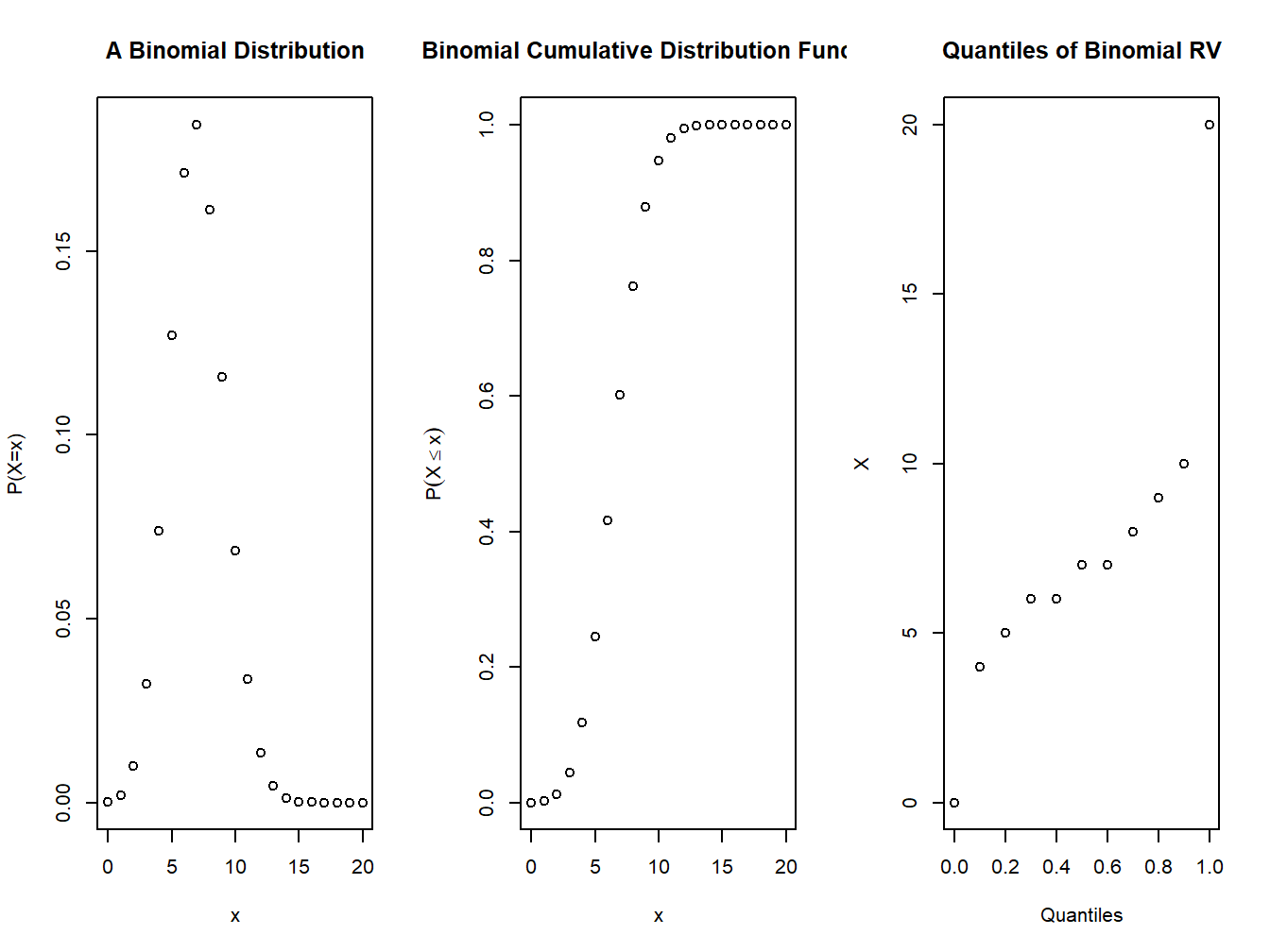

Figure 4.1: pmf and cdf of a binomial distribution

Problem 1: Find the mass function of a binomial distribution with \(n=20,\, p=0.4\). Also draw the graphs of the mass function and cumulative distribution function.

4.4.1.2 Poisson distribution

The Poisson distribution is the limiting case of a binomial distribution. The pmf of Poisson distribution is defined as:

\[p(x)=\dfrac{e^{-\lambda}\lambda^x}{x!}\] The mean and variance of a Poisson distribution with parameter \(\lambda\) is \(\lambda\) itself. In fact, the first four centralmoments of the Poisson distribution are the same! The distribution is sometimes known as the law of rare events. It has found applications in problems such as the number of mistakes on a printed page, the number of accidents on a stretch of a highway, the number of arrivals at a queueing system, etc.

Example: Given the data n=50, mean=25, use appropriate function to find the mass function of a Poisson distribution. Also draw the graphs of the mass function and cumulative distribution function.

n <-50; l <- 25
par(mfrow=c(1,3))
plot(0:n,dpois(0:n,lambda=l),xlab="x",ylab="P(X=x)", main="A Poisson Distribution")
plot(0:n,ppois(0:n,lambda=l),xlab="x",ylab=expression(P(X<=x)),main="Poisson Cumulative Distribution Function")
plot(seq(0,1,.1),qpois(seq(0,1,.1),lambda = l),xlab="Quantiles",ylab="X",main="Quantiles of Poisson RV")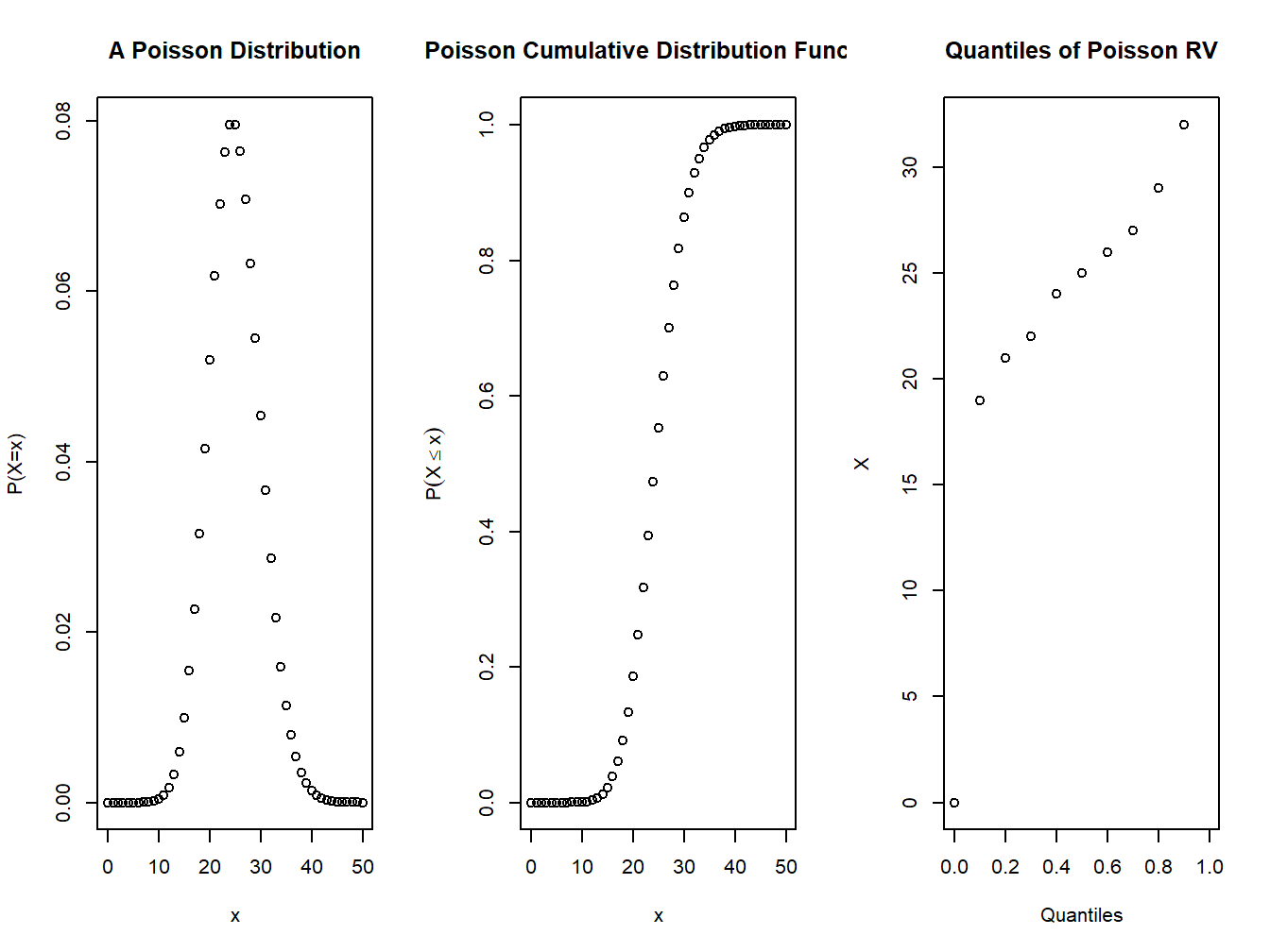

Figure 4.2: pmf and cdf of a Poisson distribution

Example: Suppose that X follows a Poisson distribution with 𝜆 = 10. Then, find its percentiles. Furthermore, the probability that X is greater than 15.

perc=qpois(seq(0,1,0.1),lambda=10)
perc

##  [1]   0   6   7   8   9  10  11  12  13  14 Inf

1-ppois(15,10) #P(X>=15)

## [1] 0.0487404

Example: The probability distribution of Poisson random variables for different 𝝀. In the previous example we saw the Poisson approximation for binomial distribution. will simply look to see what happens to the Poisson distribution for large values of 𝜆.

par(mfrow=c(2,2))
plot(0:20,dpois(0:20,lambda=2),xlab="x", ylab="Probability",type="h")
plot(0:50,dpois(0:50,lambda=5),xlab="x", ylab="Probability",type="h")
plot(0:100,dpois(0:100,lambda=20),xlab="x",ylab="Probability",type="h")
plot(0:150,dpois(0:150,lambda=110),xlab="x",ylab="Probability",type="h")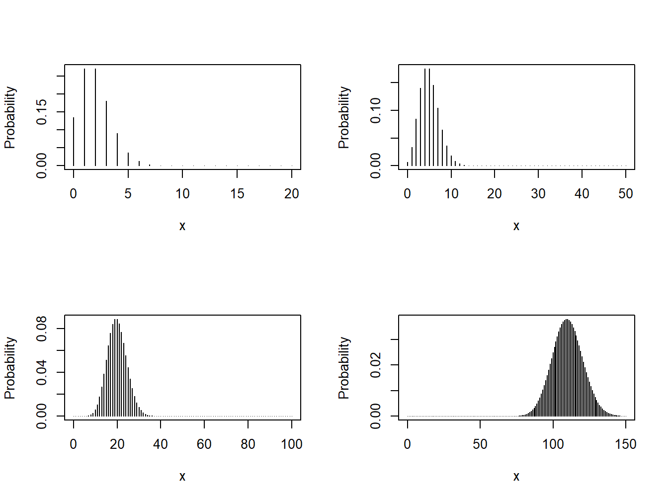

Figure 4.3: Various Poisson Distributions

4.4.2 Continuous distributions

Useful continuous distributions will be discussed here are Exponential distribution and the Normal distribution.

4.4.2.1 Exponential distribution

The pdf of the exponential distribution is defined as: \[f(x,\theta)=\frac{1}{\theta}e^{-x/\theta};\quad x>0,\theta>0\]

where \(\theta\) is the mean of the exponential distribution. In R we will pass the {}- \(\frac{1}{\theta}\) as the argument.

Example: A Simple Illustration. If the mean of the exponential distribution is 30, and we desire to compute the percentiles at the points 13, 18, 27, and 45, we obtain the required percentiles using the pexp function. Suppose, we want to know the quantiles of an exponential distribution with mean time of 30 units.

t <- c(13,18,27,45)
pexp(t,1/30) #finding the cumulative probabilities at these breaking points.

## [1] 0.3516557 0.4511884 0.5934303 0.7768698

qexp(seq(0,1,.25),1/30)

## [1]  0.000000  8.630462 20.794415 41.588831       Inf

Example:Use appropriate function to generate the pdf of the exponential distribution with mean 30 , take x values 0 to 1 with 0.25 difference. Draw the graph of the density function.

t=seq(0,1,0.25); theta=30
par(mfrow=c(1,3))
plot(t,dexp(t,rate=1/theta),xlab="x",ylab="P(X=x)", main="An Exponential Distribution")
plot(t,pexp(t,rate =1/theta),xlab="x",ylab=expression(P(X<=x)),main="Exponential Cumulative Distribution Function")
plot(t,qexp(t,rate=1/theta),xlab="Quantiles",ylab="X",main="Quantiles of exponential RV")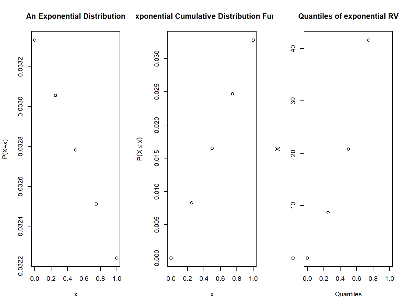

Figure 4.4: pdf and cdf of an exponential distribution

4.4.2.2 Normal distribution

The pdf of the normal distribution with mean \(\mu\) and sd \(\sigma\) is given by:

\[f(x)=\dfrac{1}{\sqrt{2\pi}\sigma}e^{-(x-\mu)^2/2\sigma^2}\] Here the parameters are \(\mu\) and \(\sigma\).

Example: Plot a normal distribution with mean 49 and sd 10 for x values from 0,100.

x=seq(0,100,5)
plot(x,dnorm(x,mean = 49,sd=10),type='l',ylab=expression(f(x)))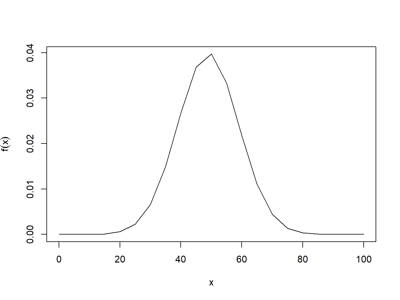

Figure 4.5: pdf of normal distribution

** Example:** Generate and draw the cdf and pdf of a normal distribution with mean=10 and standard deviation=3. Use values of \(x\) from 0 to 20 in intervals of 1.

t=seq(0,20,1); mu=10;sd=3
par(mfrow=c(1,3))
plot(t,dnorm(t,mean = mu,sd=sd),xlab="x",type='l',ylab="f(X=x)", main="A normal Distribution")
plot(t,pnorm(t,mean = mu,sd=sd),type='l',xlab="x",ylab=expression(P(X<=x)),main="normal Cumulative Distribution Function")
plot(seq(0,1,0.1),qnorm(seq(0,1,0.1),mean = mu,sd=sd),xlab="Quantiles",ylab="X",main="Quantiles of normal RV")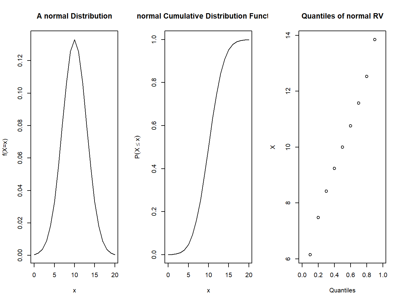

Figure 4.6: pdf and cdf of a normal distribution

Example: Some Shady Normal Curves. We will again consider a standard normal random variable, which ismore popularly denoted in Statistics by Z. Some of the much needed probabilities are \(P(Z > 0)\), \(P(−1.96 < Z < 1.96)\), etc.

par(mfrow=c(1,3))
# Probability Z Greater than 0
curve(dnorm(x,0,1),-4,4,xlab="z",ylab="f(z)")
z <- seq(0,4,0.02)
lines(z,dnorm(z),type="h",col="grey")
# 95% Coverage
curve(dnorm(x,0,1),-4,4,xlab="z",ylab="f(z)")
z <- seq(-1.96,1.96,0.001)
lines(z,dnorm(z),type="h",col="grey")
# 95% Coverage
curve(dnorm(x,0,1),-4,4,xlab="z",ylab="f(z)")
z <- seq(-2.58,2.58,0.001)
lines(z,dnorm(z),type="h",col="grey")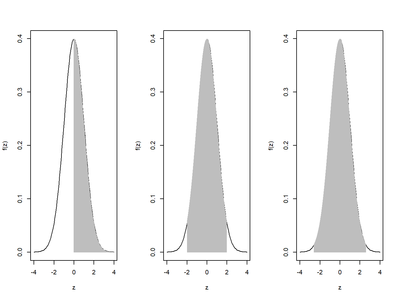

Figure 4.7: Shaded Normal Curves

4.4.2.3 Normal Approximation of Binomial Distribution Using Central Limit Theorem

Let \(\textstyle \{X_{1},\ldots ,X_{n}\}\) be a random sample of size \({\textstyle n}\) — that is, a sequence of independent and identically distributed (i.i.d.) random variables drawn from a distribution of expected value given by \(\textstyle \mu\) and finite variance given by \(\textstyle \sigma ^{2}\). Suppose we are interested in the sample average

\({\displaystyle {\bar {X}}_{n}\equiv {\frac {X_{1}+\cdots +X_{n}}{n}}}\) of these random variables. By the law of large numbers, the sample averages converge almost surely (and therefore also converge in probability) to the expected value \({\textstyle \mu }\) as \(\textstyle n\to \infty\). The classical central limit theorem describes the size and the distributional form of the stochastic fluctuations around the deterministic number \({\textstyle \mu }\) during this convergence. More precisely, it states that as \({\textstyle n}\) gets larger, the distribution of the difference between the sample average \({\textstyle {\bar {X}}_{n}}\) and its limit \({\textstyle \mu }\), when multiplied by the factor \({\textstyle {\sqrt {n}}}\) (that is \({\textstyle {\sqrt {n}}({\bar {X}}_{n}-\mu )}\)) approximates the normal distribution with mean 0 and variance \({\textstyle \sigma ^{2}}\).

The Central Limit Theorem illustrates that a sample will follow normal distribution if the sample size is large enough. We will use that as well as the rules around determining probabilities in a normal distribution, to arrive at the probability in a Binomial or Poisson case with large \(n\).

Problem 1: I have a group of 100 friends who are smokers. The probability of a random smoker having lung disease is 0.3. What are chances that a maximum of 35 people wind up with lung disease?

Solution: Here we have to find \(P(x\leq 35)\). Using a Binomial distribution we can calculate it as:

pbinom(35,size=100,prob=0.3)

## [1] 0.8839214

To use a normal distribution, first we have to find \(\mu=np=100\times 0.3=30\), \(\sigma=\sqrt{npq}=\sqrt{100\times 0.3\times 0.7}=4.582576\).

pnorm(35,30,4.582576)

## [1] 0.8623832

Problem 2: Suppose 35% of all households in Carville have three cars, what is the probability that a random sample of 80 households in Carville will contain at least 30 households that have three cars.

Solution: Here we have to find \(p(x\geq 30)\).

Using Binomial distribution,

1-pbinom(30,80,0.35)

## [1] 0.2764722

For using Normal distribution \(\mu=28,\sigma=4.266146\).

pnorm(30,28,4.27,lower.tail = F)

## [1] 0.319755

Problem 3: About two out of every three gas purchases at Cheap Gas station are paid for by credit cards. 480 customers buying gas at this station are randomly selected. Find the following probabilities using the binomial distribution, normal approximation and using the continuity correction.

1. Find n, p, q, the mean and the standard deviation.

2. Find the probability that greater than 300 will pay for their purchases using credit card.

3. Find the probability that between 220 to 320 will pay for their purchases using credit card.

4. Generate a random number using the command floor(rnorm(1, mean=200, sd=50)).

Write this number down. Lets call it N. (This number will be different for each student.)

5. Find the probability that at most N customers will pay for their purchases using credit card.

4.4.3 Fitting of distributions

Any observed distribution can be fitted to a theoretical distribution using the formula \(N\times p(X=x)\), where \(N\) is the total frequency and \(p(x)\) is the pdf of the target distribution.

Example: The following data shows the result of throwing 12 fair dice 4,096 times; a throw of 4,5, or 6 being called success.

\(\begin{array}{|l|ccccccccccccc|}\hline \text{Success(X)}:& 0 &1& 2& 3& 4 &5& 6& 7& 8& 9& 10& 11& 12\\\hline \text{Frequency(f)}:& 0 &7& 60& 198& 430& 731& 948& 847& 536& 257& 71& 11& 0\\\hline \end{array}\)

Fit a binomial distribution and find the expected frequencies. Compare the graphs of the observed frequency and theoretical frequency.

Solution:

Since we need a binomial fit, \(p(x)=\binom n x p^x (1-p)^{n-x}\). Here \(p\) is the probability for getting 4, 5 or six in one throw. So \(p=3/6\).

p=3/6
N=4096
Observed=c(0 ,7, 60,198,430,731,948,847,536, 257, 71,11, 0)
success=seq(0,12,1)
TF=round(N*dbinom(success,size=12,prob=p),2)
par(mfrow=c(1,2))
plot(success,Observed,xlab="success",ylab="f(z)")
title("Observed Distribution")
plot(success,TF,xlab="success",ylab="TF")
title("Fitted Binomial Distribution")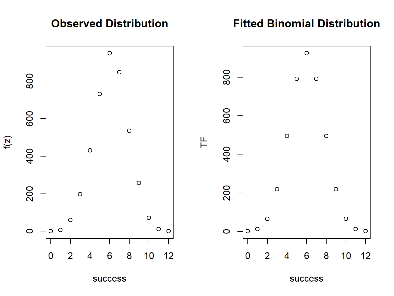

Figure 4.8: Comparison of observed and fitted distributions

The fitting table is shown in Table 4.1.

Fit=data.frame(Success=success,Observed,Fitted_binom=TF)
knitr::kable(
  Fit, caption = 'The binomial fitting table',
  booktabs = TRUE)

Table 4.1: The binomial fitting table

Success	Observed	Fitted_binom
0	0	1
1	7	12
2	60	66
3	198	220
4	430	495
5	731	792
6	948	924
7	847	792
8	536	495
9	257	220
10	71	66
11	11	12
12	0	1

References

Kerns, G. Jay. 2018. Prob: Elementary Probability on Finite Sample Spaces. https://CRAN.R-project.org/package=prob.

Statisticat, and LLC. 2021. LaplacesDemon Tutorial. Bayesian-Inference.com. https://web.archive.org/web/20150206004624/http://www.bayesian-inference.com/software.

Tattar, Prabhanjan. 2015. ACSWR: A Companion Package for the Book "a Course in Statistics with r". https://CRAN.R-project.org/package=ACSWR.

---

1. The posterior probability is calculated using the Bayes theorem, \(P(B_j|A)=\dfrac{P(A|B_j)P(B_j)}{\sum\limits_{j=1}^mP(A|B_j)P(B_j)}\)↩︎