Chapter 6 Multivariate Models

6.1 Constructing and sampling multivariate distributions

Illustrating the construction and sampling of several multivariate distributions (mostly elliptical).

Understanding the construction of multivariate normal distributions, normal variance mixtures, elliptical distributions etc.

6.1.1 Basic ‘ingredients’

Building a covariance/correlation matrix

Covariance matrix:

A = matrix(c(4, 0,
              1, 1), ncol = 2, byrow = TRUE) # Cholesky factor of the ...
(Sigma = A %*% t(A)) # ... symmetric, positive definite (covariance) matrix Sigma

##      [,1] [,2]
## [1,]   16    4
## [2,]    4    2

Corresponding correlation matrix:

(P = outer(1:2, 1:2, Vectorize(function(r, c)
    Sigma[r,c]/(sqrt(Sigma[r,r])*sqrt(Sigma[c,c]))))) # construct the corresponding correlation matrix

##              [,1]         [,2]
## [1,] 1.0000000000 0.7071067812
## [2,] 0.7071067812 1.0000000000

(P.  = cov2cor(Sigma)) # for a more elegant solution, see the source of cov2cor()

##              [,1]         [,2]
## [1,] 1.0000000000 0.7071067812
## [2,] 0.7071067812 1.0000000000

stopifnot(all.equal(P., P))

Another option would be as.matrix(Matrix::nearPD(Sigma, corr = TRUE, maxit = 1000)$mat) which works differently, though (by finding a correlation matrix close to the given matrix in the Frobenius norm) and thus gives a different answer.

Decomposing a covariance/correlation matrix

We frequently need to decompose a covariance matrix $\Sigma$ (or correlation matrix $P$) as $\Sigma = A A^\top$. To this end there are several possibilities.

The Cholesky decomposition:

A. = t(chol(Sigma)) # the Cholesky factor (lower triangular with real entries > 0)
stopifnot(all.equal(A. %*% t(A.) , Sigma), # checking decomposition
          all.equal(A., A)) # checking uniqueness of the Cholesky decomposition

Other decompositions of $\Sigma$ than A %*% t(A) are possible, too:

if(FALSE) {
    ## Eigendecomposition (or spectral decomposition)
    eig = eigen(Sigma) # eigenvalues and eigenvectors
    V = eig$vectors # matrix of eigenvectors
    Lambda = diag(pmax(eig$values, 0))
    stopifnot(all.equal(Sigma, V %*% Lambda %*% t(V))) # for real, symmetric matrices
    A.eig = V %*% sqrt(Lambda) %*% t(V)
    Sigma.eig = A.eig %*% t(A.eig)
    stopifnot(all.equal(Sigma.eig, Sigma))
    ## ... but A.. (non-triangular) and A (triangular) are different

    ## Singular-value decomposition
    sv = svd(Sigma) # singular values, U, V (left/right singular vectors) such that Sigma = U diag(<singular values>) V^T
    A.sv = sv$u %*% sqrt(diag(pmax(sv$d, 0))) %*% t(sv$v)
    Sigma.sv = A.sv %*% t(A.sv)
    stopifnot(all.equal(Sigma.sv, Sigma))
}

6.1.2 Sampling from the multivariate normal distribution

Sampling $Z$ ($\text{iid } \mathcal{N}(0,1)$)

n = 1000 # sample size
d = 2 # dimension
set.seed(271) # set a seed (for reproducibility)
Z = matrix(rnorm(n * d), ncol = d) # sample iid N(0,1) random variates
mabs = max(abs(Z))
lim = c(-mabs, mabs)
plot(Z, xlim = lim, ylim = lim,
     xlab = expression(Z[1]), ylab = expression(Z[2]))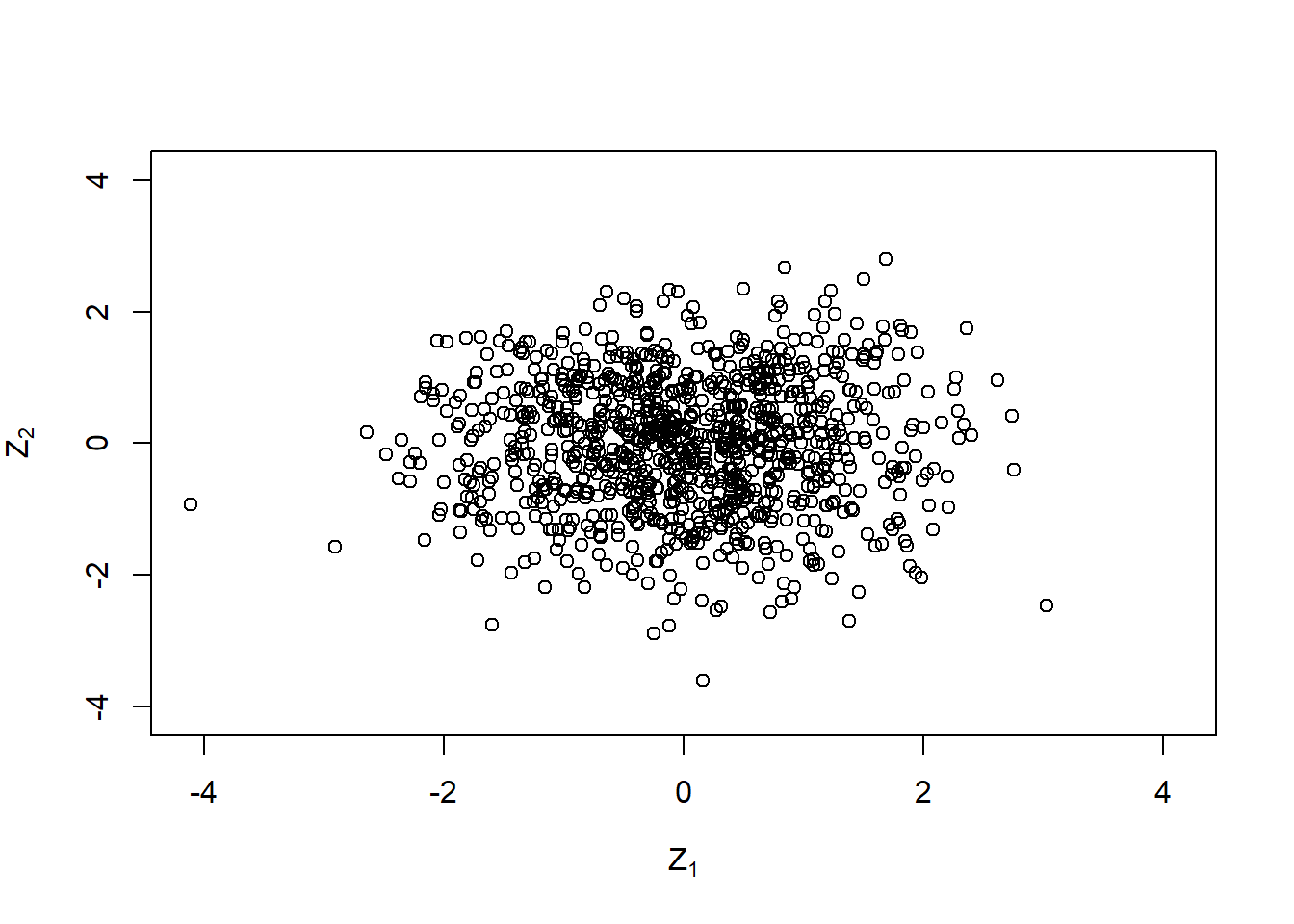

Change the covariance matrix from identity to $\Sigma$:

X. = t(A %*% t(Z)) # ~ N_d(0, Sigma)
xlim = c(-16, 16)
ylim = c(-8, 8)
plot(X., xlim = xlim, ylim = ylim,
     xlab = expression(X[1]), ylab = expression(X[2]))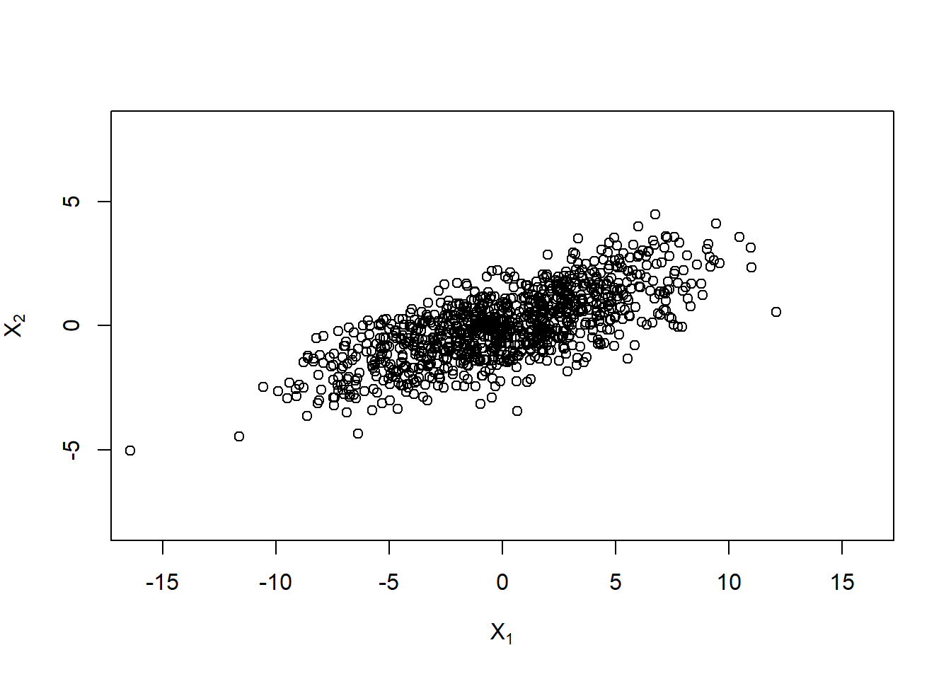

Use a shift to get $X \sim \mathcal{N}_d(\mu, \Sigma)$:

mu = c(1, 3)
X.norm = rep(mu, each = n) + X.
plot(X.norm, xlim = xlim, ylim = ylim,
     xlab = expression(X[1]), ylab = expression(X[2]))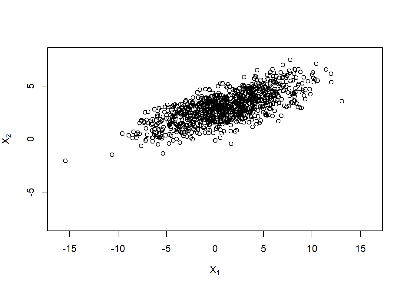

## Think about why the rep() and why the t()'s above!

Plot (even larger correlation):

P. = matrix(c(   1, 0.95,
               0.95, 1), ncol = d, byrow = TRUE)
Sigma. = outer(1:d, 1:d, Vectorize(function(r, c)
                P.[r,c] * (sqrt(Sigma[r,r])*sqrt(Sigma[c,c])))) # construct the corresponding Sigma
## Note: When manually changing the off-diagonal entry of Sigma make sure that
##       |Sigma.[1,2]| <= sqrt(Sigma.[1,1]) * sqrt(Sigma.[2,2]) still holds
A. = t(chol(Sigma.)) # new Cholesky factor
X.norm. = rep(mu, each = n) + t(A. %*% t(Z)) # generate the sample
plot(rbind(X.norm, X.norm.), xlim = xlim, ylim = ylim,
     xlab = expression(X[1]), ylab = expression(X[2]),
     col = rep(c("black", "royalblue3"), each = n))
legend("bottomright", bty = "n", pch = c(1,1), col = c("black", "royalblue3"),
       legend = c(expression(N(mu,Sigma)),
                  expression("With larger absolute correlation")))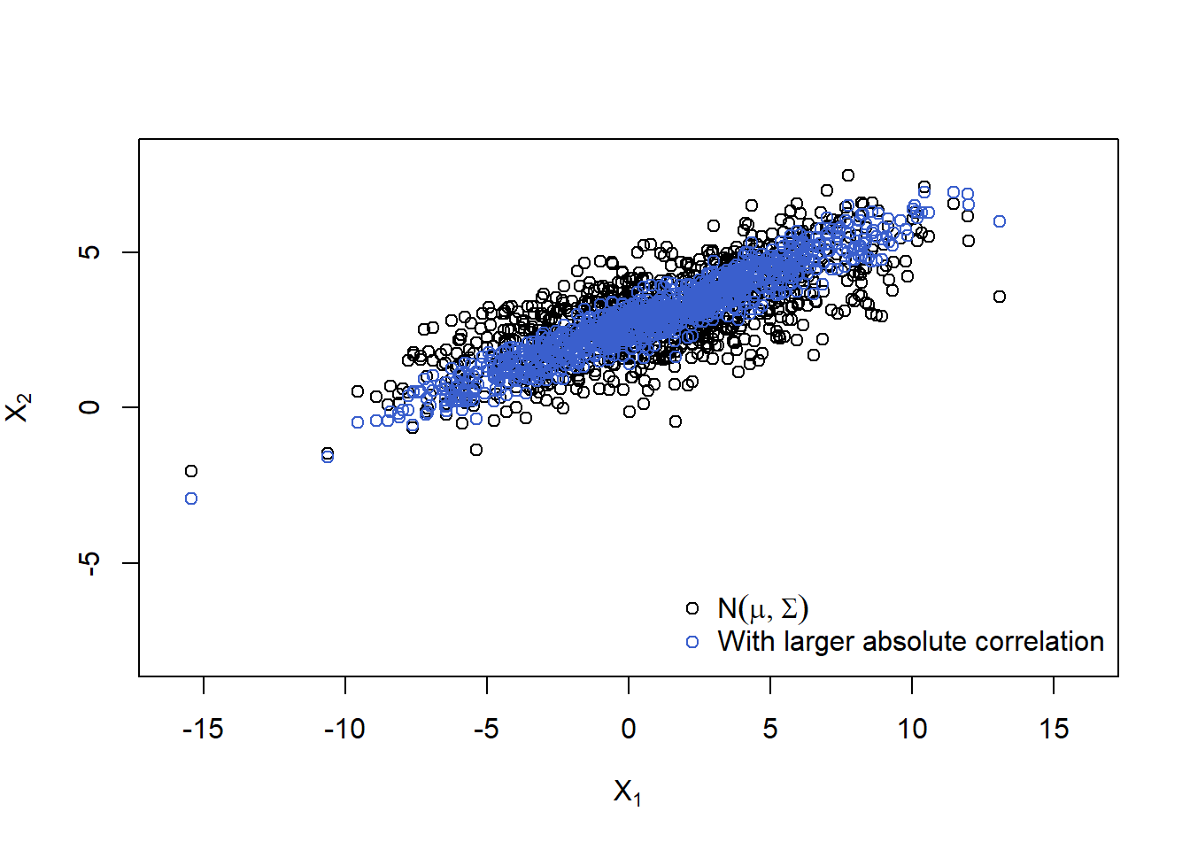

Plot (switch sign of correlation):

Sigma. = Sigma * matrix(c( 1, -1,
                           -1,  1), ncol = d, byrow = TRUE)
A. = t(chol(Sigma.))
X.norm. = rep(mu, each = n) + t(A. %*% t(Z))
plot(rbind(X.norm, X.norm.), xlim = xlim, ylim = ylim,
     xlab = expression(X[1]), ylab = expression(X[2]),
     col = rep(c("black", "royalblue3"), each = n))
legend("bottomright", bty = "n", pch = c(1,1), col = c("black", "royalblue3"),
       legend = c(expression(N(mu,Sigma)),
                  expression("Correlation sign switched")))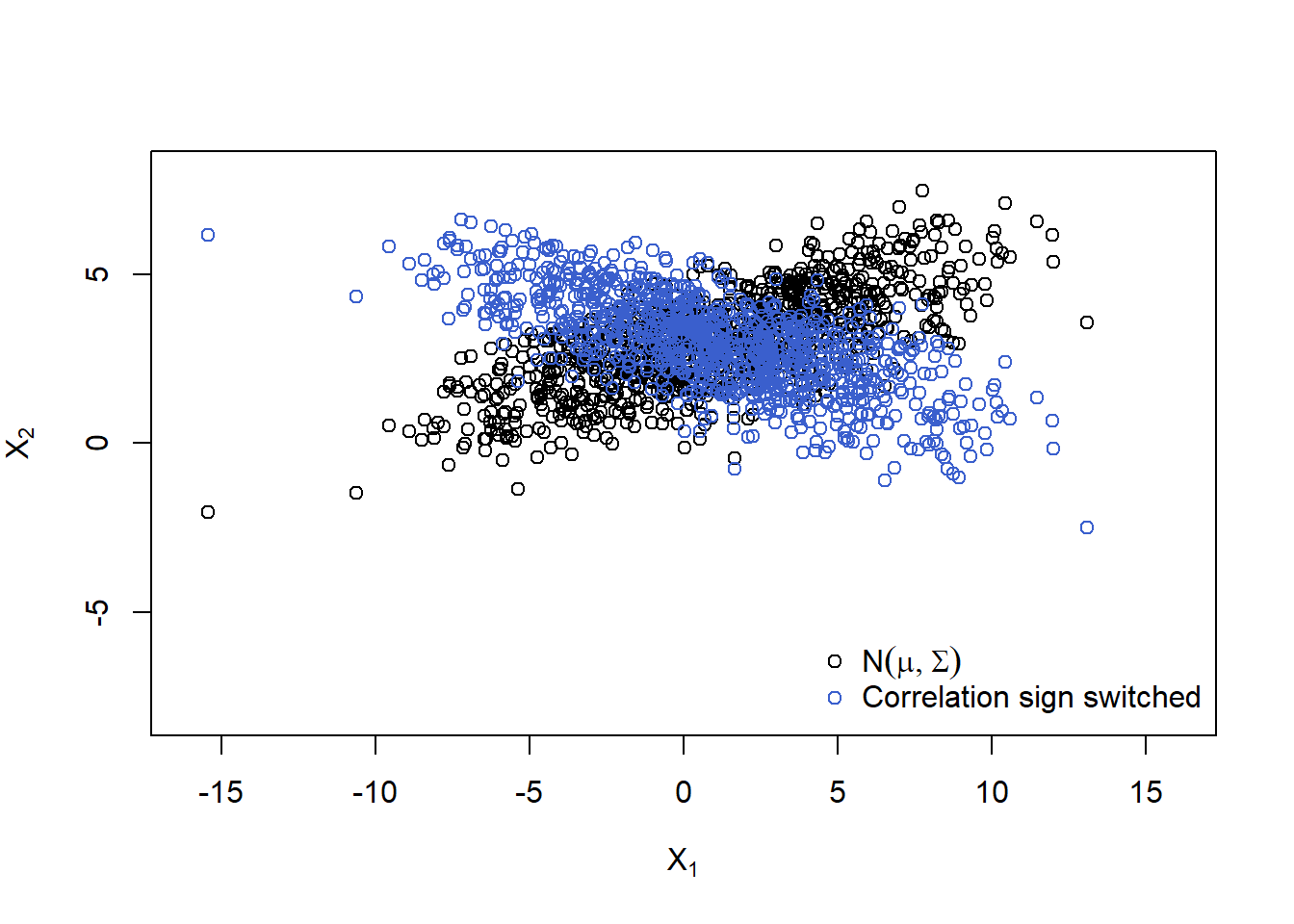

## Note: This has all been done based on the same Z (and we also recycle it below)!

6.1.3 Sampling from the multiv. $t$ distribution (and other normal variance mixtures)

Definition 6.1 (multivariate normal variance mixture distribution) The random vector $\boldsymbol{X}$ is said to have a (multivariate) normal variance mixture distribution if \[ \boldsymbol{X} \stackrel{d}{=} \boldsymbol{\mu} + \sqrt{W}A \boldsymbol{Z}, \] where

$\boldsymbol{Z} \sim \mathcal{N}_k(\boldsymbol{0}, I_k)$ ;
$W \geq 0$ is a non-negative, scalar-valued rv that is independent of $\boldsymbol{Z}$, and
$A \in \mathbb{R}^{d \times k}$ and $\boldsymbol{\mu} \in \mathbb{R}^d$ are a matrix and a vector of constants, respectively.

MFE (2015, Definition 6.4)

$\blacksquare$

A sample from a multivariate $t_\nu$ distribution

Example 6.1 (multivariate $t$ distribution) If we take $W$ to be an rv with an inverse gamma distribution $W \sim \operatorname{Ig}\left(\frac{1}{2} \nu, \frac{1}{2} \nu \right)$ (which is equivalent to saying that $\nu/W \sim \chi_{\nu}^{2}$), then $\boldsymbol{X}$ has a multivariate $t$ distribution with $\nu$ degrees of freedom. Our notation for the multivariate $t$ is $\boldsymbol{X} \sim t_{d}(\nu, \boldsymbol{\mu}, \Sigma)$, and we note that $\Sigma$ is not the covariance matrix of $\boldsymbol{X}$ in this definition of the multivariate $t$. Since $E(W)=\nu /(\nu-2)$ we have $\operatorname{cov}(\boldsymbol{X})=(\nu /(\nu-2)) \Sigma$, and the covariance matrix (and correlation matrix ) of this distribution is only defined if $\nu>2$.

MFE (2015, Example 6.7)

$\blacksquare$

nu = 3 # degrees of freedom
set.seed(314)
W = 1/rgamma(n, shape = nu/2, rate = nu/2) # mixture variable for a multiv. t_nu distribution
plot(W, log = "y")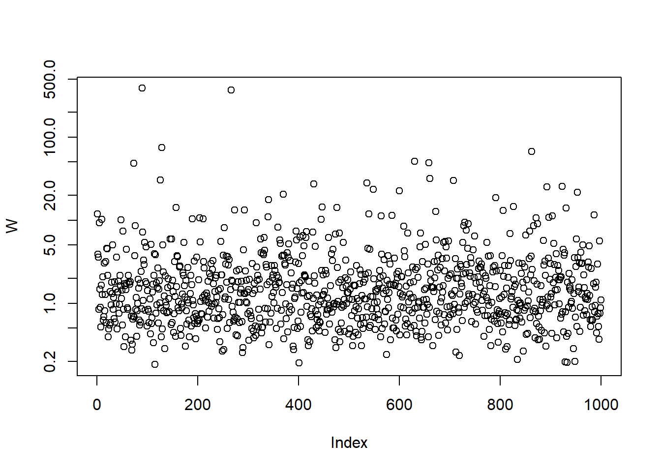

X.t = rep(mu, each = n) + sqrt(W) * t(A %*% t(Z))
xlim = c(-40, 80)
ylim = c(-20, 60)
plot(rbind(X.t, X.norm), xlim = xlim, ylim = ylim,
     xlab = expression(X[1]), ylab = expression(X[2]),
     col = rep(c("maroon3", "black"), each = n))
legend("bottomright", bty = "n", pch = c(1,1), col = c("black", "maroon3"),
       legend = c(expression(N(mu,Sigma)),
                  expression(italic(t)[nu](mu,Sigma))))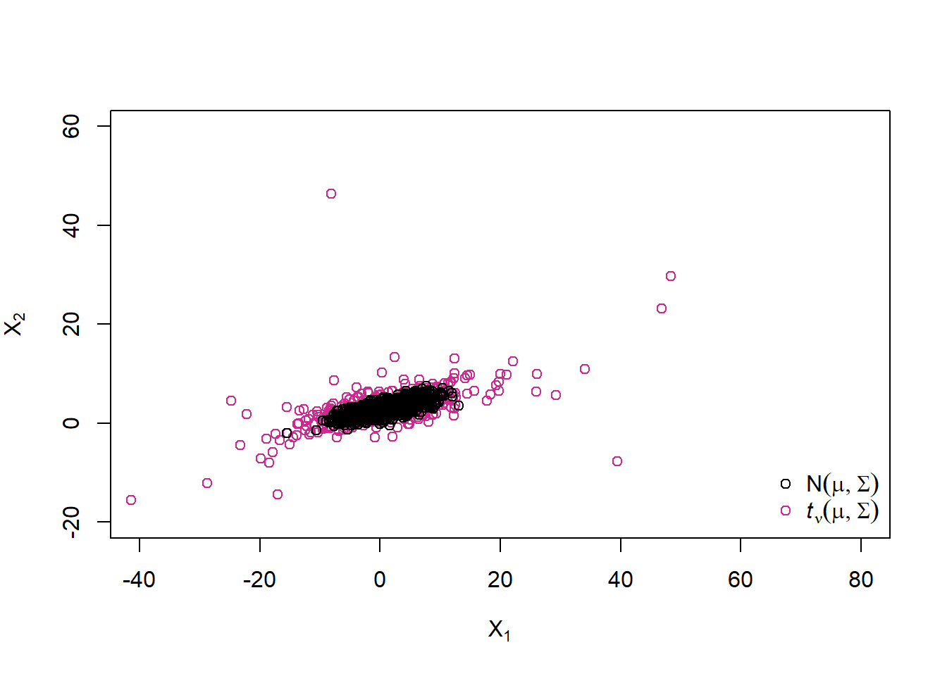

A 2-point distribution for $W$ (= two ‘overlaid’ multiv. normals)

Let’s change the distribution of $W$ to a 2-point distribution with $W = 1$ with prob. $0.5$ and $W = 2$ with prob. $0.5$. What we will see are two ‘overlaid’ normal distributions (as each of $W = 1$ and $W = 2$ corresponds to one).

W.binom = 1 + rbinom(n, size = 1, prob = 0.5)
cols = rep("royalblue3", n)
cols[W.binom == 2] = "maroon3"
X.W.binom = rep(mu, each = n) + sqrt(W.binom) * t(A %*% t(Z))
plot(rbind(X.t, X.W.binom), xlab = expression(X[1]), ylab = expression(X[2]),
     col = c(rep("black", n), cols))
legend("topright", bty = "n", pch = rep(1, 3), col = c("royalblue3", "maroon3", "black"),
       legend = c(expression(N(mu,W*Sigma)~"for W = 1"),
                  expression(N(mu,W*Sigma)~"for W = 2"),
                  expression(italic(t)[nu](mu,Sigma))))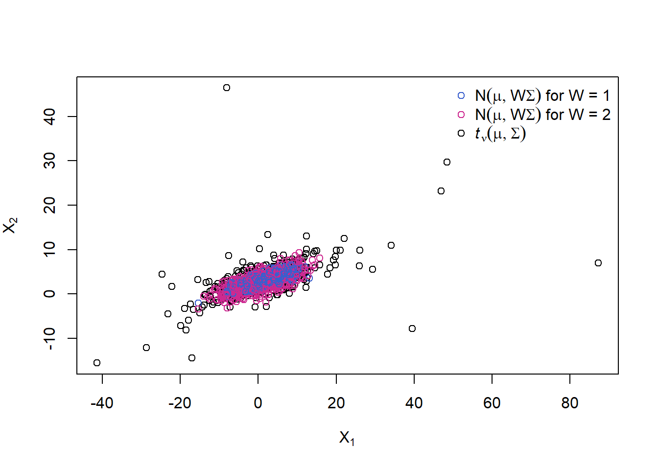

With probability 0.5 we sample from a normal variance mixture with $W = 1$ and with probability 0.5 we sample from one with $W = 2$. By using a df for W with infinite upper endpoint, we can reach further out in the tails than with any multivariate normal distribution by overlaying normals with different (unbounded) covariance matrices (and this is what is creating heavier tails for the $t$ distribution than the normal).

An uncorrelated multivariate $t_\nu$ distribution vs an independent one

A. = diag(sqrt(diag(Sigma))) # Cholesky factor of the diagonal matrix containing the variances
X.t.uncor = rep(mu, each = n) + sqrt(W) * t(A. %*% t(Z)) # uncorrelated t samples
X.t.ind   = rep(mu, each = n) + matrix(rt(n * d, df = nu), ncol = d) # independent t samples
plot(rbind(X.t.uncor, # uncorrelated t; dependence only introduced by sqrt(W) => shifted spherical distribution
           X.t, # full t; dependence introduced by sqrt(W) *and* correlation
           X.t.ind), # independence
     xlim = xlim, ylim = ylim,
     xlab = expression(X[1]), ylab = expression(X[2]),
     col = rep(c("royalblue3", "maroon3", "black"), each = n))
legend("topright", bty = "n", pch = rep(1, 3), col = c("black", "royalblue3", "maroon3"),
       legend = c(expression("Independent"~italic(t)[nu]),
                  expression("Uncorrelated"~italic(t)[nu]~"(shifted spherical)"),
                  expression(italic(t)[nu](mu,Sigma))))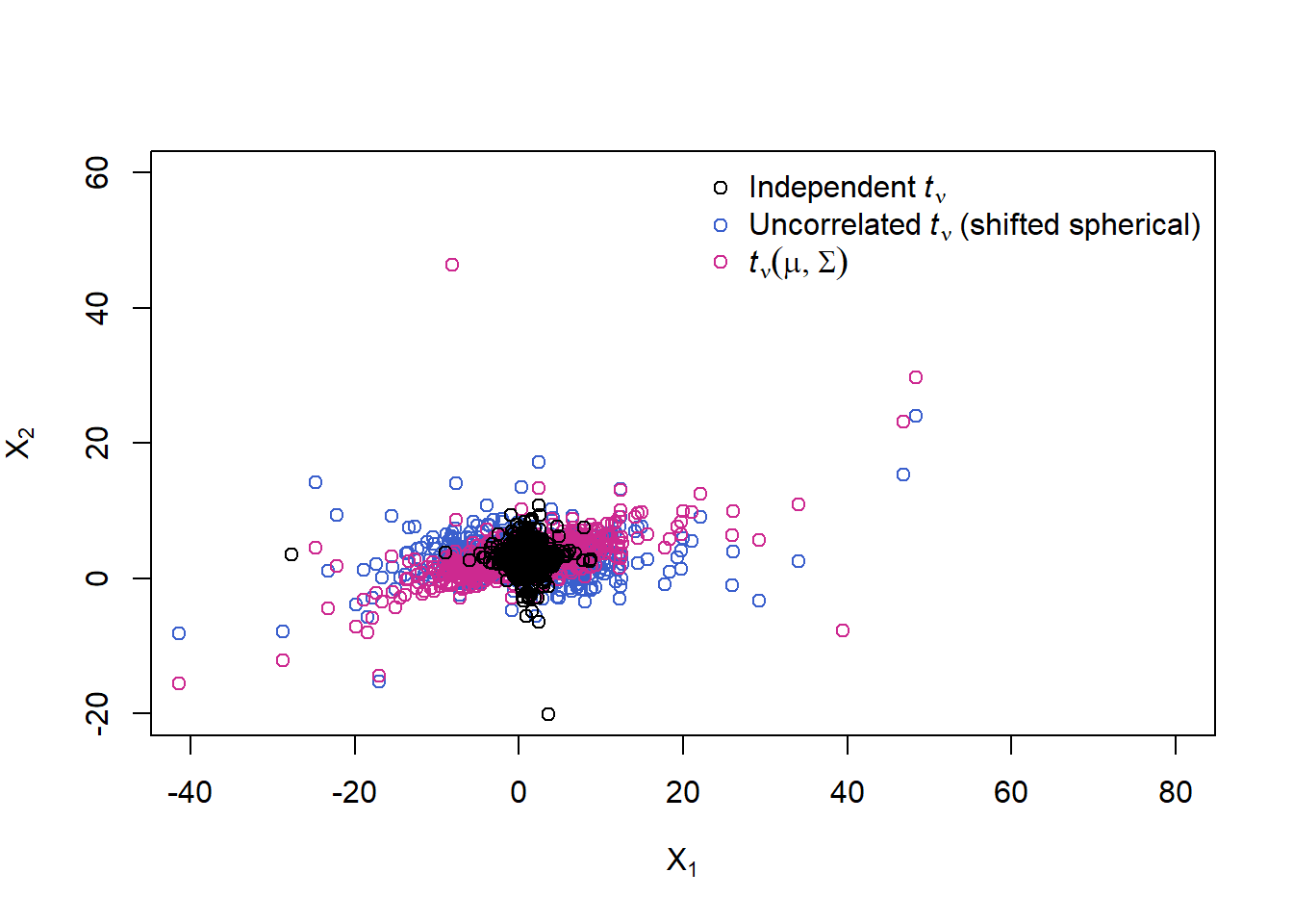

The uncorrelated (but not independent) samples show more mass in the joint tails than the independent samples. The (neither uncorrelated nor independent) $t$ samples show the most mass in the joint tails.

A normal mean-variance mixture

The models we now introduce attempt to add some asymmetry to the class of normal mixtures by mixing normal distributions with different means as well as different variances; this yields the class of multivariate normal mean–variance mixtures.

Definition 6.2 () The random vector $\boldsymbol{X}$ is said to have a (multivariate) normal mean–variance mixture distribution if \[ \boldsymbol{X} \stackrel{d}{=} \boldsymbol{m}(W) + \sqrt{W}A \boldsymbol{Z}, \] where

$\boldsymbol{Z} \sim \mathcal{N}_k(\boldsymbol{0}, I_k)$ ;
$W \geq 0$ is a non-negative, scalar-valued rv that is independent of $\boldsymbol{Z}$, and
$A \in \mathbb{R}^{d \times k}$ is a matrix, and
$\boldsymbol{m} : [0, \infty) \rightarrow \mathbb{R}^d$ is a measurable function.

In this case we have that \[ \boldsymbol{X} \mid W=w \sim \mathcal{N}_{d}(\boldsymbol{m}(w), w \Sigma) \] where $\Sigma=A A^{\prime}$ and it is clear why such distributions are known as mean-variance mixtures of normals. In general, such distributions are not elliptical.

A possible concrete specification for the function $\boldsymbol{m}(W)$ is \[ \boldsymbol{m}(W)=\boldsymbol{\mu}+W \boldsymbol{\gamma} \] where $\boldsymbol{\mu}$ and $\gamma$ are parameter vectors in $\mathbb{R}^{d}$.

MFE (2015, Definition 6.11)

$\blacksquare$

Now let’s also ‘mix’ the mean (replace $\boldsymbol{\mu}$ by $\boldsymbol{m}(W)$), to get a normal mean-variance mixture; here: choosing between two different locations $\boldsymbol{\mu}$ depending on $W$.

mu. = t(sapply(W.binom, function(w) mu + if(w == 1) 0 else c(15, 0)))
X.mean.var = mu. + sqrt(W.binom) * t(A %*% t(Z))
plot(rbind(X.W.binom, X.mean.var), xlab = expression(X[1]), ylab = expression(X[2]),
     col = c(rep("black", n), cols))
legend("topleft", bty = "n", pch = rep(1, 3), col = c("black", "royalblue3", "maroon3"),
       legend = c(expression(N(mu,W*Sigma)~"for W"%in%"{1,2}"),
                  "Mean-var. mix for W = 1",
                  "Mean-var. mix for W = 2"))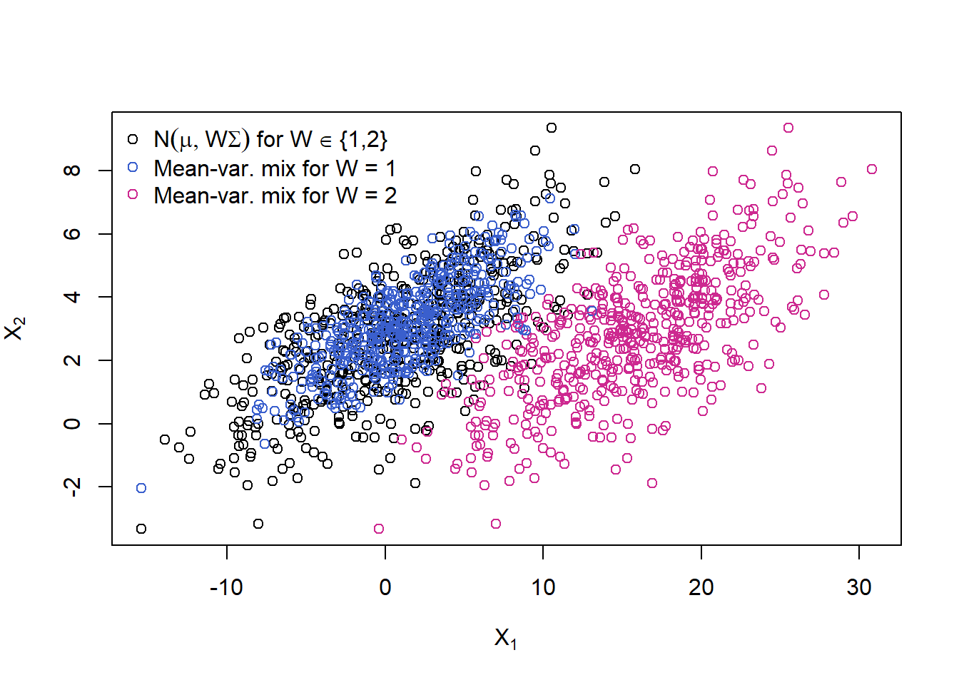

Not only do the red points show more variation, they also have a different ocation; clearly, this sample (blue + red points together) is not elliptically distributed anymore.

6.2 Fitting a multivariate normal and $t$

Fitting a multivariate normal and $t$ distribution to negative log-returns of the five components of the Dow Jones index.

library(xts) # for time series manipulation
library(nvmix) # for rNorm(), fitStudent(), rStudent()
library(qrmdata) # for Dow Jones constituents data
library(qrmtools) # for returns()

Load and extract the data we work with and plot:

data(DJ_const)
str(DJ_const)

## An 'xts' object on 1962-01-02/2015-12-31 containing:
##   Data: num [1:13595, 1:30] NA NA NA NA NA NA NA NA NA NA ...
##  - attr(*, "dimnames")=List of 2
##   ..$ : NULL
##   ..$ : chr [1:30] "AAPL" "AXP" "BA" "CAT" ...
##   Indexed by objects of class: [Date] TZ: UTC
##   xts Attributes:  
## List of 2
##  $ src    : chr "yahoo"
##  $ updated: POSIXct[1:1], format: "2016-01-03 03:51:40"

S = DJ_const['2000-01-01/', c("AAPL", "BA", "INTC", "IBM", "NKE")]
## => We work with Apple, Boeing, Intel, IBM, Nike since 2000-01-01 here
plot.zoo(S, xlab = "Time t")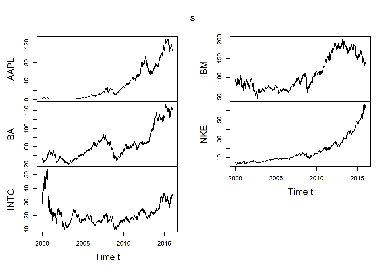

Build and plot $-$log-returns:

X = -returns(S) # compute -log-returns
pairs(as.matrix(X), main = "Scatter plot matrix of risk-factor changes", gap = 0, pch = ".")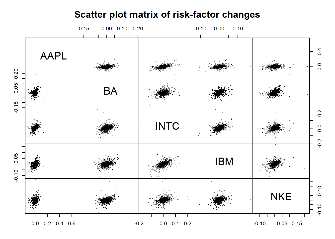

plot.zoo(X, xlab = "Time t", main = "")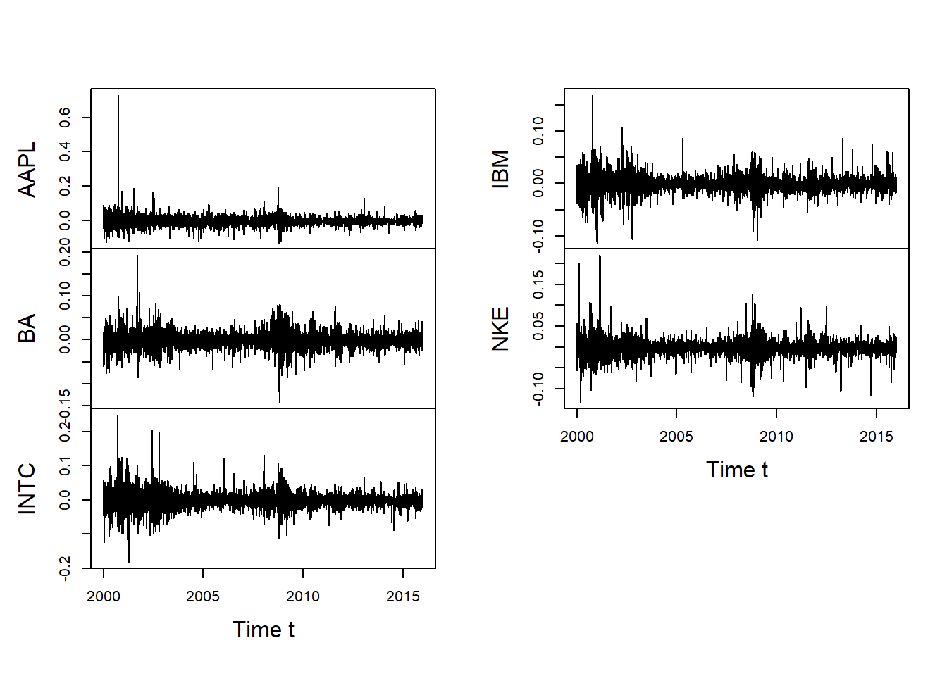

## For illustration purposes, we treat this data as realizations of iid
## five-dimensional random vectors.

Fitting a multivariate normal distribution to $\boldsymbol{X}$ and simulating from it:

mu = colMeans(X) # estimated location vector
Sigma = cov(X) # estimated scale matrix
stopifnot(all.equal(Sigma, var(X)))
P = cor(X) # estimated correlation matrix
stopifnot(all.equal(P, cov2cor(Sigma)))
n = nrow(X) # sample size
set.seed(271)
X.norm = rNorm(n, loc = mu, scale = Sigma) # N(mu, Sigma) samples

Fitting a multivariate $t$ distribution to $\boldsymbol{X}$:

fit = fitStudent(X) # fit a multivariate t distribution
X.t = rStudent(n, df = fit$df, loc = fit$loc, scale = fit$scale) # t_nu samples

Plot (sample from fitted $t$ (red), original sample (black), sample from fitted normal (blue)):

dat = rbind(t = X.t, original = as.matrix(X), norm = X.norm)
cols = rep(c("royalblue3", "black", "maroon3"), each = n)
pairs(dat, gap = 0, pch = ".", col = cols)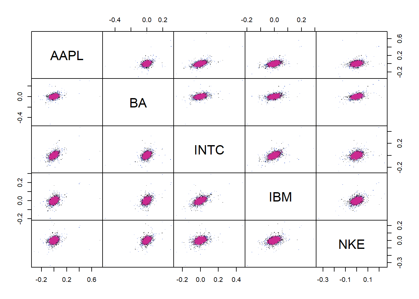

Pick out one pair (to better see that multivariate $t$ fits better):

plot(dat[,1:2], col = cols) # => the multivariate normal generates too few extreme losses!
legend("bottomright", bty = "n", pch = rep(1, 3), col = c("black", "maroon3", "royalblue3"),
       legend = c("-Log-returns", expression("Simulated fitted"~N(mu,Sigma)),
                  expression("Simulated fitted"~italic(t)[nu](mu,Sigma))))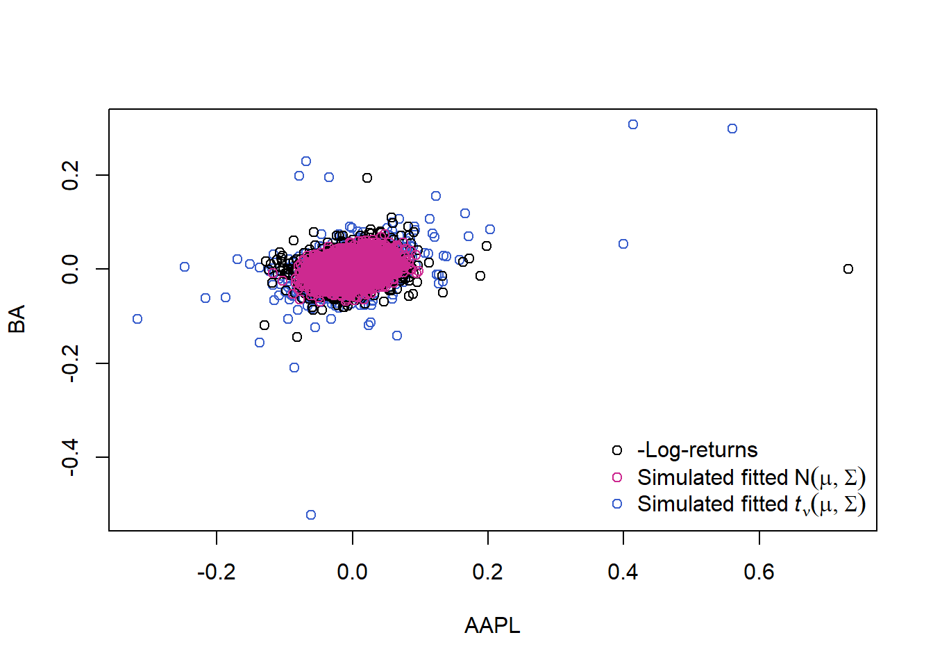

6.3 Testing multivariate normality

library(qrmtools)
library(nvmix) # for rNorm() and rStudent()
library(moments) # for jarque.test()
library(xts) # for time-series related functions

6.3.1 Generate data

n = 1000 # sample size
d = 3 # dimension
mu = 1:d # location vector
sd = sqrt(1:d) # standard deviations for scale matrix
tau = 0.5 # (homogeneous) Kendall's tau
rho = sin(tau * pi/2) # (homogeneous) correlation coefficient
Sigma = matrix(rho, nrow = d, ncol = d) # scale matrix
diag(Sigma) = rep(1, d) # => now Sigma is a correlation matrix
Sigma = Sigma * (sd %*% t(sd)) # covariance matrix
nu = 3 # degrees of freedom
set.seed(271) # set seed (for reproducibility)
X.N = rNorm(n, loc = mu, scale = Sigma) # sample from N(mu, Sigma)
X.t = rStudent(n, df = nu, loc = mu, scale = ((nu-2)/nu) * Sigma) # sample from t_d(nu, mu, ((nu-2)/nu) * Sigma) (same covariance as N(mu, Sigma))
X.t.N = sapply(1:d, function(j) qnorm(rank(X.t[,j]) / (nrow(X.t) + 1),
                                       mean = mu[j], sd = sqrt(Sigma[j, j]))) # t dependence with normal margins; see Chapter 7
if(FALSE) {
    cov(X.N)
    cov(X.t)
    ## => quite apart, but closer for larger n
}

6.3.2 Testing for $\mathcal{N}(\boldsymbol{\mu}, \Sigma)$

We treat $\boldsymbol{\mu}$ and $\Sigma$ as unknown and estimate them:

mu.N = mean(X.N)
mu.t = mean(X.t)
Sig.N = cov(X.N)
Sig.t = cov(X.t)

6.3.3 For $\mathcal{N}(\boldsymbol{\mu}, \Sigma)$ data

Formal tests

## Univariate normality
stopifnot(apply(X.N, 2, function(x) shapiro.test(x)$p.value) > 0.05) # Shapiro--Wilk
stopifnot(apply(X.N, 2, function(x) jarque.test(x) $p.value) > 0.05) # Jarque--Bera
## Note: Careful with 'multiple testing'

## Joint normality
ADmaha2 = maha2_test(X.N) # Anderson--Darling test of squared Mahalanobis distances being chi_d^2
mardiaK = mardia_test(X.N) # Mardia's kurtosis test of joint normality based on squared Mahalanobis distances
mardiaS = mardia_test(X.N, type = "skewness") # Mardia's skewness test of joint normality based on Mahalanobis angles
stopifnot(mardiaS$p.value > 0.05, mardiaK$p.value > 0.05, ADmaha2$p.value > 0.05)

Graphical tests

## Univariate normality
qq_plot(X.N[,1], FUN = qnorm, method = "empirical") # margin 1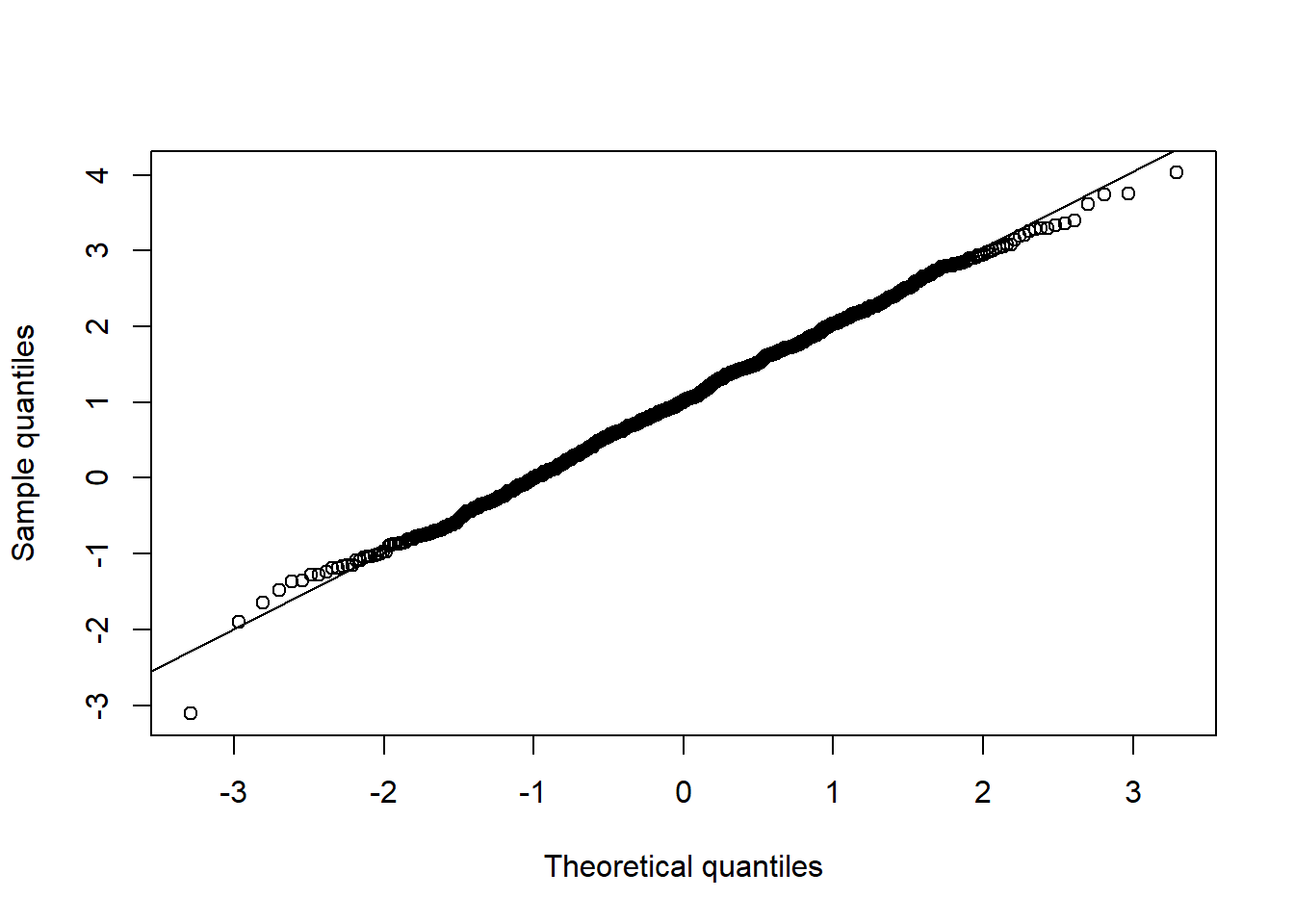

qq_plot(X.N[,2], FUN = qnorm, method = "empirical") # margin 2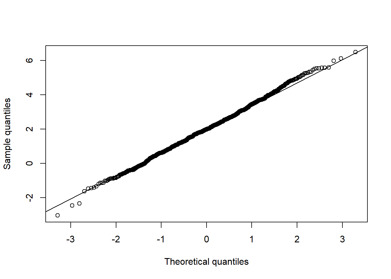

qq_plot(X.N[,3], FUN = qnorm, method = "empirical") # margin 3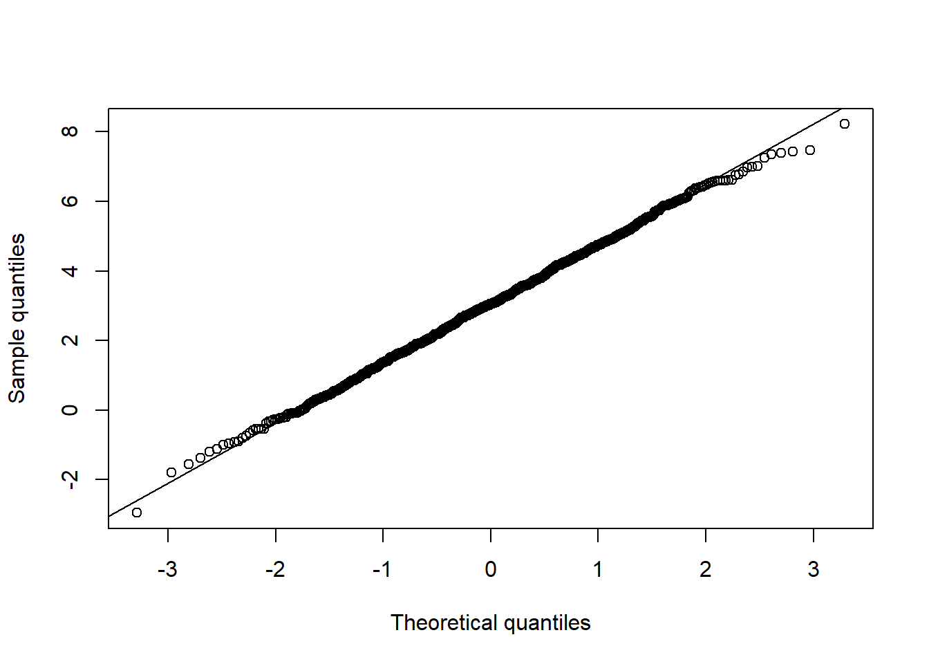

## Joint normality
pairs(X.N, gap = 0, pch = ".") # visual assessment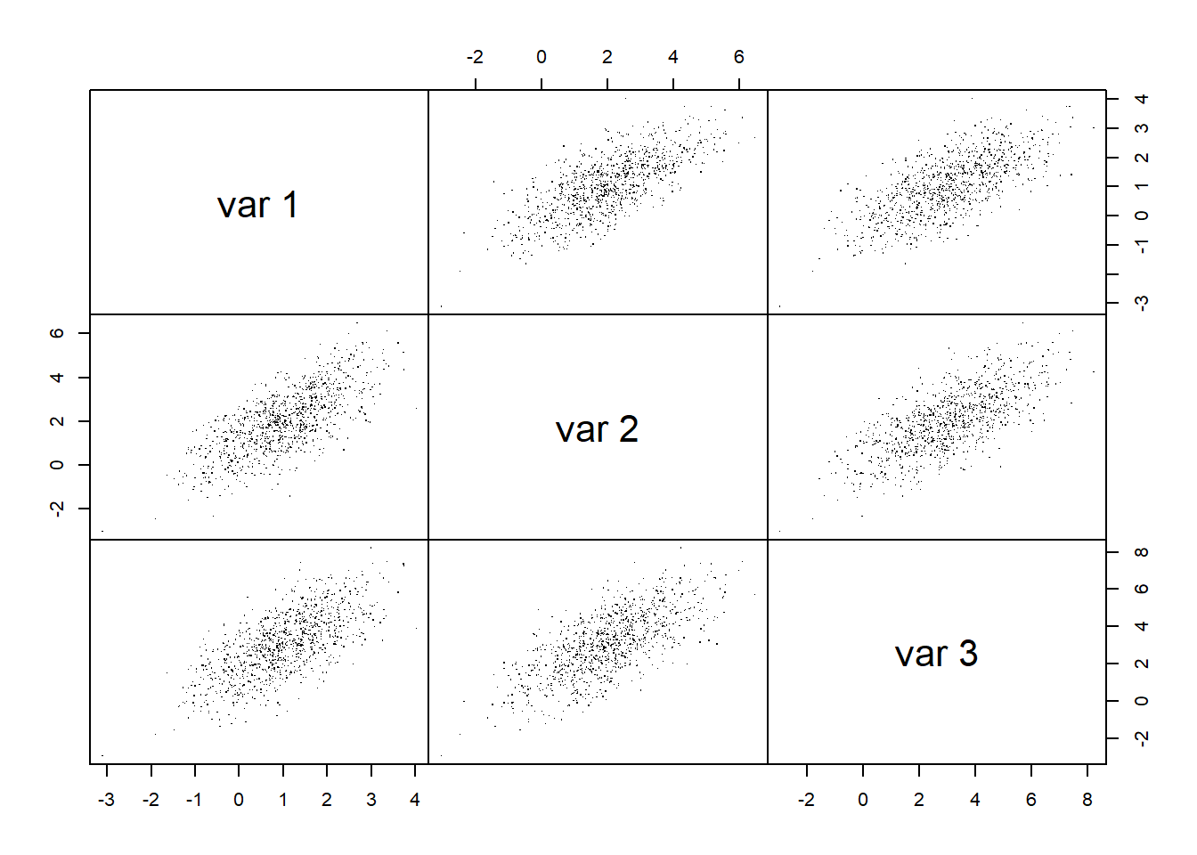

D2.d = mahalanobis(X.N, center = colMeans(X.N), cov = cov(X.N)) # squared Mahalanobis distances
qq_plot(D2.d, FUN = function(p) qchisq(p, df = d)) # => no significant departure visible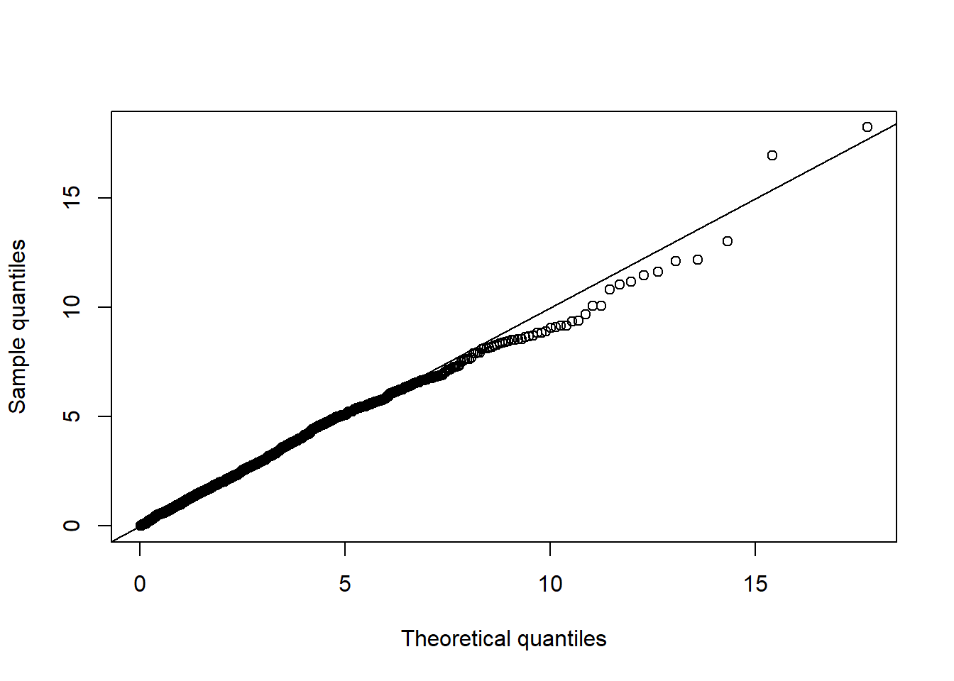

6.3.4 For $t_d(\nu, \boldsymbol{\mu}, \Sigma)$ data

Formal tests

## Univariate normality
stopifnot(apply(X.t, 2, function(x) shapiro.test(x)$p.value) <= 0.05) # Shapiro--Wilk
stopifnot(apply(X.t, 2, function(x) jarque.test(x) $p.value) <= 0.05) # Jarque--Bera
## Note: Careful with 'multiple testing'

## Joint normality
ADmaha2 = maha2_test(X.t) # Anderson--Darling test of squared Mahalanobis distances being chi_d^2
mardiaK = mardia_test(X.t) # Mardia's kurtosis test of joint normality based on squared Mahalanobis distances
mardiaS = mardia_test(X.t, type = "skewness") # Mardia's skewness test of joint normality based on Mahalanobis angles
stopifnot(mardiaS$p.value <= 0.05, mardiaK$p.value <= 0.05, ADmaha2$p.value <= 0.05)

Graphical tests

## Univariate normality
qq_plot(X.t[,1], FUN = qnorm, method = "empirical") # margin 1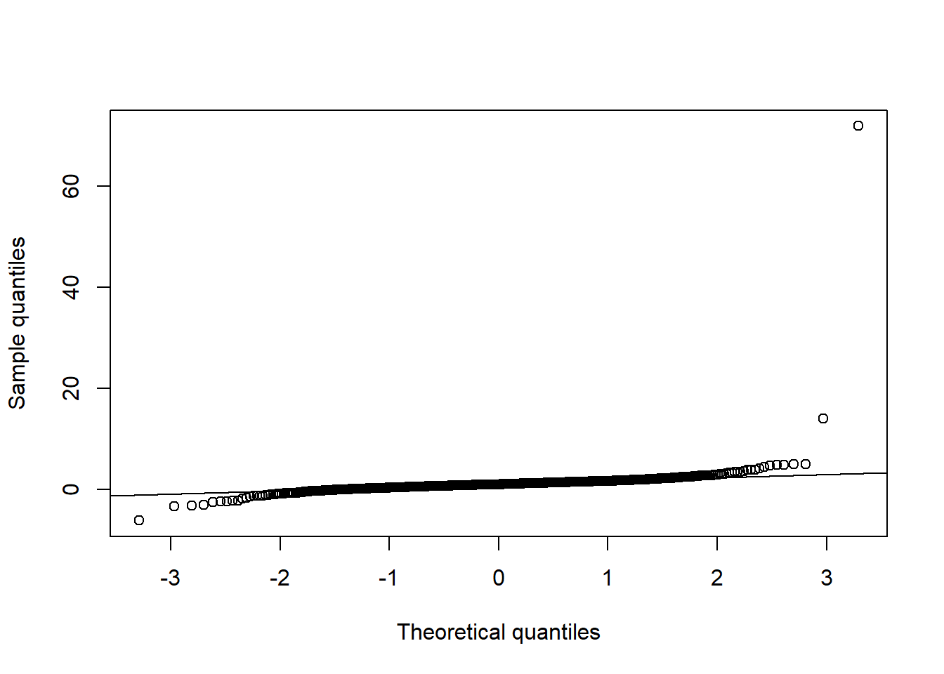

qq_plot(X.t[,2], FUN = qnorm, method = "empirical") # margin 2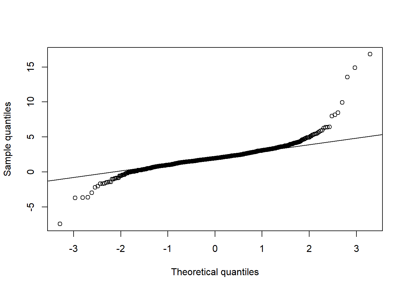

qq_plot(X.t[,3], FUN = qnorm, method = "empirical") # margin 3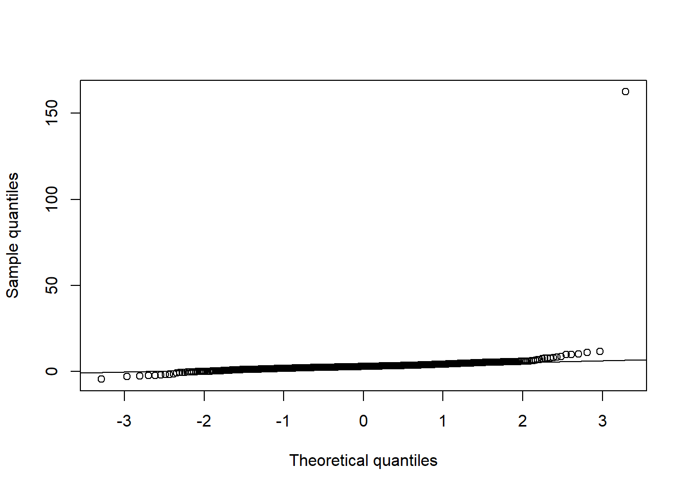

## Joint normality
pairs(X.t, gap = 0, pch = ".") # visual assessment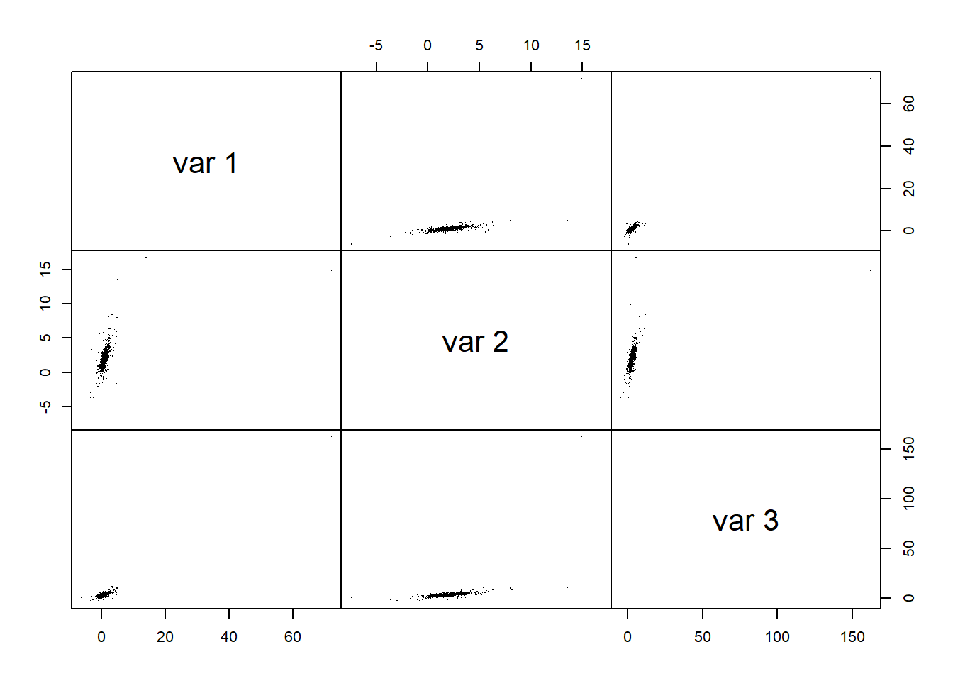

D2.d = mahalanobis(X.t, center = colMeans(X.t), cov = cov(X.t)) # squared Mahalanobis distances
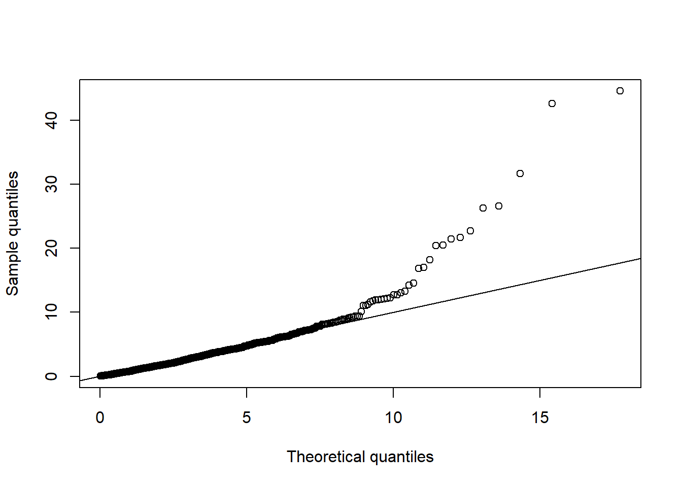
qq_plot(D2.d, FUN = function(p) qchisq(p, df = d)) # => departure clearly visible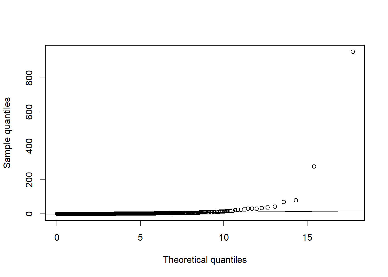

6.3.5 For $t_d(\nu, 0, P)$ dependence but $\mathcal{N}(0, 1)$ margins

Formal tests

## Univariate normality
stopifnot(apply(X.t.N, 2, function(x) shapiro.test(x)$p.value) > 0.05) # Shapiro--Wilk
stopifnot(apply(X.t.N, 2, function(x) jarque.test(x) $p.value) > 0.05) # Jarque--Bera

## Joint normality
ADmaha2 = maha2_test(X.t.N) # Anderson--Darling test of squared Mahalanobis distances being chi_d^2
mardiaK = mardia_test(X.t.N) # Mardia's kurtosis test of joint normality based on squared Mahalanobis distances
mardiaS = mardia_test(X.t.N, type = "skewness") # Mardia's skewness test of joint normality based on Mahalanobis angles
stopifnot(mardiaS$p.value <= 0.05, mardiaK$p.value <= 0.05, ADmaha2$p.value <= 0.05)

Graphical tests

## Univariate normality
qq_plot(X.t.N[,1], FUN = qnorm, method = "empirical") # margin 1

qq_plot(X.t.N[,2], FUN = qnorm, method = "empirical") # margin 2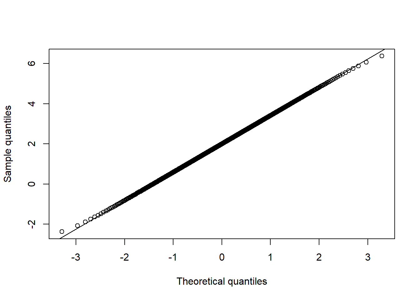

qq_plot(X.t.N[,3], FUN = qnorm, method = "empirical") # margin 3

## Joint normality
pairs(X.t.N, gap = 0, pch = ".") # visual assessment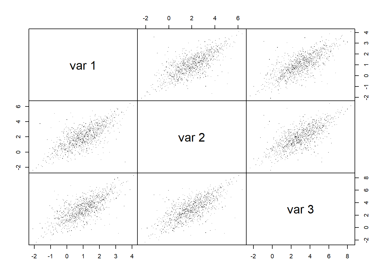

D2.d = mahalanobis(X.t.N, center = colMeans(X.t.N), cov = cov(X.t.N)) # squared Mahalanobis distances
qq_plot(D2.d, FUN = function(p) qchisq(p, df = d)) # => departure clearly visible

R Notes for QRM

Chapter 6 Multivariate Models

6.1 Constructing and sampling multivariate distributions

6.1.1 Basic ‘ingredients’

Building a covariance/correlation matrix

Decomposing a covariance/correlation matrix

6.1.2 Sampling from the multivariate normal distribution

6.1.3 Sampling from the multiv. \(t\) distribution (and other normal variance mixtures)

A sample from a multivariate \(t_\nu\) distribution

A 2-point distribution for \(W\) (= two ‘overlaid’ multiv. normals)

An uncorrelated multivariate \(t_\nu\) distribution vs an independent one

A normal mean-variance mixture

6.2 Fitting a multivariate normal and \(t\)

6.3 Testing multivariate normality

6.3.1 Generate data

6.3.2 Testing for \(\mathcal{N}(\boldsymbol{\mu}, \Sigma)\)

6.3.3 For \(\mathcal{N}(\boldsymbol{\mu}, \Sigma)\) data

Formal tests

Graphical tests

6.3.4 For \(t_d(\nu, \boldsymbol{\mu}, \Sigma)\) data

Formal tests

Graphical tests

6.3.5 For \(t_d(\nu, 0, P)\) dependence but \(\mathcal{N}(0, 1)\) margins

Formal tests

Graphical tests