Chapter 4 Financial Time Series
As a general notational convention in this section and the remainder of the chapter we will denote white noise by \((\varepsilon_t)_{t\in \mathbb{Z}}\) and strict white noise by \((Z_t)_{t \in \mathbb{Z}}\).
4.1 Review
Definition 4.1 (martingale difference) The time series \(\left(X_{t}\right)_{t \in \mathbb{Z}}\) is known as a martingale-difference sequence with respect to the filtration \(\left(\mathcal{F}_{t}\right)_{t \in \mathbb{Z}}\) if \(E\left|X_{t}\right|<\infty\), \(X_{t}\) is \(\mathcal{F}_{t}\) -measurable (adapted) and \[ E\left(X_{t} \mid \mathcal{F}_{t-1}\right)=0, \quad \forall t \in \mathbb{Z} \] Obviously the unconditional mean of such a process is also zero: \[ E\left(X_{t}\right)=E\left(E\left(X_{t} \mid \mathcal{F}_{t-1}\right)\right)=0, \quad \forall t \in \mathbb{Z} \] Moreover, if \(E\left(X_{t}^{2}\right)<\infty\) for all \(t\), then autocovariances satisfy \[ \begin{aligned} \gamma(t, s) &=E\left(X_{t} X_{s}\right) \\ &=\left\{\begin{array}{ll} E\left(E\left(X_{t} X_{s} \mid \mathcal{F}_{s-1}\right)\right)=E\left(X_{t} E\left(X_{s} \mid \mathcal{F}_{s-1}\right)\right)=0, & t<s \\ E\left(E\left(X_{t} X_{s} \mid \mathcal{F}_{t-1}\right)\right)=E\left(X_{s} E\left(X_{t} \mid \mathcal{F}_{t-1}\right)\right)=0, & t>s \end{array}\right. \end{aligned} \] Thus a finite-variance martingale-difference sequence has zero mean and zero covariance. If the variance is constant for all \(t\), it is a white noise process.
MFE (2015, Definition 4.6)\(\blacksquare\)
Definition 4.2 (ARMA process) Let \((\varepsilon_t)_{t\in \mathbb{Z}}\) be \(WN(0,\sigma^2_\varepsilon)\). The process \((X_t)_{t\in \mathbb{Z}}\) is a zero-mean \(\text{ARMA}(p, q)\) process if it is a covariance-stationary process satisfying difference equations of the form \[ X_{t}-\phi_{1} X_{t-1}-\cdots-\phi_{p} X_{t-p}=\varepsilon_{t}+\theta_{1} \varepsilon_{t-1}+\cdots+\theta_{q} \varepsilon_{t-q}, \quad \forall t \in \mathbb{Z} \] \(\left(X_{t}\right)\) is an ARMA process with mean \(\mu\) if the centred series \(\left(X_{t}-\mu\right)_{t \in \mathbb{Z}}\) is a zeromean \(\text{ARMA}(p, q)\) process.
MFE (2015, Definition 4.7)\(\blacksquare\)
Whether the process is strictly stationary or not will depend on the exact nature of the driving white noise, also known as the process of innovations. If the innovations are iid, or themselves form a strictly stationary process, then the ARMA process will also be strictly stationary.
4.1.1 Models for the conditional mean
In practice, the models we fit to real data will be both invertible and causal solutions of the ARMA-defining equations.
Consider a general invertible ARMA model with non-zero mean. For what comes later it will be useful to observe that we can write such models as \[ X_{t}=\mu_{t}+\varepsilon_{t}, \quad \mu_{t}=\mu+\sum_{i=1}^{p} \phi_{i}\left(X_{t-i}-\mu\right)+\sum_{j=1}^{q} \theta_{j} \varepsilon_{t-j} \] Since we have assumed invertibility, the terms \(\varepsilon_{t-j}\), and hence \(\mu_{t}\), can be written in terms of the infinite past of the process up to time \(t-1\) ; \(\mu_{t}\) is said to be measurable with respect to \(\mathcal{F}_{t-1}=\sigma\left(\left\{X_{s}: s \leqslant t-1\right\}\right)\).
If we make the assumption that the white noise \(\left(\varepsilon_{t}\right)_{t \in \mathbb{Z}}\) is a martingale-difference sequence with respect to \(\left(\mathcal{F}_{t}\right)_{t \in \mathbb{Z}}\), then \(E\left(X_{t} \mid \mathcal{F}_{t-1}\right)=\mu_{t}\). In other words, such an ARMA process can be thought of as putting a particular structure on the conditional mean \(\mu_{t}\) of the process. ARCH and GARCH processes will later be seen to put structure on the conditional variance \(Var\left(X_{t} \mid \mathcal{F}_{t-1}\right)\).
4.1.2 ARCH (autoregressive conditionally heteroscedastic) process
Definition 4.3 (ARCH process) Let \(\left(Z_{t}\right)_{t \in \mathbb{Z}}\) be \(\operatorname{SWN}(0,1) .\) The process \(\left(X_{t}\right)_{t \in \mathbb{Z}}\) is an \(\operatorname{ARCH}(p)\) process if it is strictly stationary and if it satisfies, for all \(t \in \mathbb{Z}\) and some strictly positive-valued process \(\left(\sigma_{t}\right)_{t \in \mathbb{Z}}\), the equations \[ \begin{aligned} X_{t}&=\sigma_{t} Z_{t} \\ \sigma_{t}^{2}&=\alpha_{0}+\sum_{i=1}^{p} \alpha_{i} X_{t-i}^{2} \end{aligned} \] where \(\alpha_{0}>0\) and \(\alpha_{i} \geqslant 0, i=1, \ldots, p\)
MFE (2015, Definition 4.16)\(\blacksquare\)
If we simply assume that the process is a covariance-stationary white noise (for which we will give a condition in Proposition 4.1), then \(E\left(X_{t}^{2}\right)<\infty\) and \[ \operatorname{var}\left(X_{t} \mid \mathcal{F}_{t-1}\right)=E\left(\sigma_{t}^{2} Z_{t}^{2} \mid \mathcal{F}_{t-1}\right)=\sigma_{t}^{2} \operatorname{var}\left(Z_{t}\right)=\sigma_{t}^{2} \] Thus the model has the interesting property that its conditional standard deviation \(\sigma_{t}\), or volatility, is a continually changing function of the previous squared values of the process.
The name ARCH refers to this structure: the model is autoregressive, since \(X_t\) clearly depends on previous \(X_{t−i}\) , and conditionally heteroscedastic, since the conditional variance changes continually.
Proposition 4.1 (stationarity of \(\text{ARCH}(1)\)) The \(\text{ARCH}(1)\) process is a covariance-stationary white noise process if and only if \(\alpha_1 < 1\). The variance of the covariance-stationary process is given by \(\alpha_0/(1 − \alpha_1)\).
MFE (2015, Proposition 4.18)\(\blacksquare\)
4.1.3 GARCH (generalized ARCH) process
Definition 4.4 (GARCH process) Let \(\left(Z_{t}\right)_{t \in \mathbb{Z}}\) be \(\operatorname{SWN}(0,1)\). The process \(\left(X_{t}\right)_{t \in \mathbb{Z}}\) is a \(\text{GARCH}(p, q)\) process if it is strictly stationary and if it satisfies, for all \(t \in \mathbb{Z}\) and some strictly positive-valued process \(\left(\sigma_{t}\right)_{t \in \mathbb{Z}}\), the equations \[ X_{t}=\sigma_{t} Z_{t}, \quad \sigma_{t}^{2}=\alpha_{0}+\sum_{i=1}^{p} \alpha_{i} X_{t-i}^{2}+\sum_{j=1}^{q} \beta_{j} \sigma_{t-j}^{2} \] where \(\alpha_{0}>0, \alpha_{i} \geq 0, i=1, \ldots, p\), and \(\beta_{j} \geq 0, j=1, \ldots, q\).
MFE (2015, Definition 4.20)\(\blacksquare\)
The GARCH processes are generalized ARCH processes in the sense that the squared volatility \(\sigma_{t}^{2}\) is allowed to depend on previous squared volatilities, as well as previous squared values of the process.
Proposition 4.2 (stationarity of \(\text{GARCH}(1,1)\)) The \(\text{GARCH}(1, 1)\) process is a covariance-stationary white noise process if and only if \(\alpha_{1}+\beta_{1}<1\). The variance of the covariance-stationary process is given by \(\alpha_{0} /\left(1-\alpha_{1}-\beta_{1}\right)\).
MFE (2015, Proposition 4.21)\(\blacksquare\)
Definition 4.5 (ARMA models with GARCH errors) Let \(\left(Z_{t}\right)_{t \in \mathbb{Z}}\) be \(\operatorname{SWN}(0,1)\). The process \(\left(X_{t}\right)_{t \in \mathbb{Z}}\) is said to be an \(\text{ARMA} \left(p_{1}, q_{1}\right)\) process with \(\text{GARCH}\left(p_{2}, q_{2}\right)\) errors if it is covariance stationary and satisfies difference equations of the form \[ \begin{aligned} X_{t}&=\mu_{t}+\sigma_{t} Z_{t} \\ \mu_{t}&=\mu+\sum_{i=1}^{p_{1}} \phi_{i}\left(X_{t-i}-\mu\right)+\sum_{j=1}^{q_{1}} \theta_{j}\left(X_{t-j}-\mu_{t-j}\right) \\ \sigma_{t}^{2}&=\alpha_{0}+\sum_{i=1}^{p_{2}} \alpha_{i}\left(X_{t-i}-\mu_{t-i}\right)^{2}+\sum_{j=1}^{q_{2}} \beta_{j} \sigma_{t-j}^{2} \end{aligned} \] where \(\alpha_{0}>0, \alpha_{i} \geqslant 0, i=1, \ldots, p_{2}, \beta_{j} \geqslant 0, j=1, \ldots, q_{2}\), and \(\sum_{i=1}^{p_{2}} \alpha_{i}+\sum_{j=1}^{q_{2}} \beta_{j}<1\)
MFE (2015, Definition 4.22)\(\blacksquare\)
4.2 GARCH simulation
Simulating paths, extracting components and plotting of a \(\text{GARCH}(1,1)\) model.
library(rugarch)##
## Attaching package: 'rugarch'## The following object is masked from 'package:stats':
##
## sigmalibrary(qrmtools)4.2.1 Specify the \(\text{GARCH}(1,1)\) model
\(\text{GARCH}(1,1)\) model specification:
(uspec = ugarchspec(variance.model = list(model = "sGARCH", # standard GARCH
                                           garchOrder = c(1, 1)), # GARCH(1,1)
                     mean.model = list(armaOrder = c(0, 0), # no ARMA part
                                       include.mean = FALSE), # no mean included
                     distribution.model = "norm", # normal innovations
                     fixed.pars = list(omega = 0.02, # cond. var. constant (= alpha_0)
                                       alpha1 = 0.15, # alpha_1
                                       beta1 = 0.8))) # beta_1
##
## *---------------------------------*
## * GARCH Model Spec *
## *---------------------------------*
##
## Conditional Variance Dynamics
## ------------------------------------
## GARCH Model : sGARCH(1,1)
## Variance Targeting : FALSE
##
## Conditional Mean Dynamics
## ------------------------------------
## Mean Model : ARFIMA(0,0,0)
## Include Mean : FALSE
## GARCH-in-Mean : FALSE
##
## Conditional Distribution
## ------------------------------------
## Distribution : norm
## Includes Skew : FALSE
## Includes Shape : FALSE
## Includes Lambda : FALSE4.2.2 Generate paths from a specified model
Generate two realizations of length 2000:
m = 2 # number of paths
n = 2000 # sample size
set.seed(271) # set seed (for reproducibility)
(paths = ugarchpath(uspec, n.sim = n, n.start = 50, # burn-in sample size
                     m.sim = m))
##
## *------------------------------------*
## * GARCH Model Path Simulation *
## *------------------------------------*
## Model: sGARCH
## Horizon: 2000
## Simulations: 2
## Seed Sigma2.Mean Sigma2.Min Sigma2.Max Series.Mean Series.Min
## sim1 NA 0.422 0.119 4.43 0.000382 -3.80
## sim2 NA 0.353 0.131 1.87 0.002134 -2.50
## Mean(All) 0 0.388 0.125 3.15 0.001258 -3.15
## Unconditional NA 0.400 NA NA 0.000000 NA
## Series.Max
## sim1 3.10
## sim2 2.75
## Mean(All) 2.92
## Unconditional NAstr(paths) # S4 object of class 'uGARCHpath'## Formal class 'uGARCHpath' [package "rugarch"] with 3 slots
## ..@ path :List of 3
## .. ..$ sigmaSim : num [1:2000, 1:2] 0.459 0.437 0.457 0.453 0.429 ...
## .. ..$ seriesSim: num [1:2000, 1:2] -0.1402 -0.488 -0.346 -0.0421 -0.0622 ...
## .. ..$ residSim : num [1:2000, 1:2] -0.1402 -0.488 -0.346 -0.0421 -0.0622 ...
## ..@ model:List of 10
## .. ..$ modelinc : Named num [1:22] 0 0 0 0 0 0 1 1 1 0 ...
## .. .. ..- attr(*, "names")= chr [1:22] "mu" "ar" "ma" "arfima" ...
## .. ..$ modeldesc :List of 3
## .. .. ..$ distribution: chr "norm"
## .. .. ..$ distno : int 1
## .. .. ..$ vmodel : chr "sGARCH"
## .. ..$ modeldata : list()
## .. ..$ pars : num [1:19, 1:6] 0 0 0 0 0 0 0.02 0.15 0.8 0 ...
## .. .. ..- attr(*, "dimnames")=List of 2
## .. .. .. ..$ : chr [1:19] "mu" "ar" "ma" "arfima" ...
## .. .. .. ..$ : chr [1:6] "Level" "Fixed" "Include" "Estimate" ...
## .. ..$ start.pars: NULL
## .. ..$ fixed.pars:List of 3
## .. .. ..$ omega : num 0.02
## .. .. ..$ alpha1: num 0.15
## .. .. ..$ beta1 : num 0.8
## .. ..$ maxOrder : num 1
## .. ..$ pos.matrix: num [1:21, 1:3] 0 0 0 0 0 0 1 2 3 0 ...
## .. .. ..- attr(*, "dimnames")=List of 2
## .. .. .. ..$ : chr [1:21] "mu" "ar" "ma" "arfima" ...
## .. .. .. ..$ : chr [1:3] "start" "stop" "include"
## .. ..$ fmodel : NULL
## .. ..$ pidx : num [1:19, 1:2] 1 2 3 4 5 6 7 8 9 10 ...
## .. .. ..- attr(*, "dimnames")=List of 2
## .. .. .. ..$ : chr [1:19] "mu" "ar" "ma" "arfima" ...
## .. .. .. ..$ : chr [1:2] "begin" "end"
## ..@ seed : int NAstr(paths@path) # simulated processes X_t, volatilities sigma_t and unstandardized residuals epsilon_t## List of 3
## $ sigmaSim : num [1:2000, 1:2] 0.459 0.437 0.457 0.453 0.429 ...
## $ seriesSim: num [1:2000, 1:2] -0.1402 -0.488 -0.346 -0.0421 -0.0622 ...
## $ residSim : num [1:2000, 1:2] -0.1402 -0.488 -0.346 -0.0421 -0.0622 ...We can use getClass() to see more information about such objects:
getClass("uGARCHpath")## Class "uGARCHpath" [package "rugarch"]
##
## Slots:
##
## Name: path model seed
## Class: vector vector integer
##
## Extends:
## Class "GARCHpath", directly
## Class "rGARCH", by class "GARCHpath", distance 2We can also use getSlots() to see the composition:
getSlots("uGARCHpath")## path model seed
## "vector" "vector" "integer"## EXERCISE: Try simulating paths with different innovation distributions (e.g. Student t)4.2.3 Plotting uGARCHpath objects
Extract the simulated series:
X = fitted(paths) # simulated process X_t = mu_t + epsilon_t for epsilon_t = sigma_t * Z_t
sig = sigma(paths) # volatilities sigma_t (conditional standard deviations)
eps = paths@path$residSim # unstandardized residuals epsilon_t = sigma_t * Z_t
## Note: There are no extraction methods for the unstandardized residuals epsilon_t
## Sanity checks (=> fitted() and sigma() grab out the right quantities)
stopifnot(all.equal(X,   paths@path$seriesSim, check.attributes = FALSE),
          all.equal(sig, paths@path$sigmaSim,  check.attributes = FALSE))
Plot the simulated paths (\(X_t\)):
plot(X[,1], type = "l", ylab = expression(X[1]))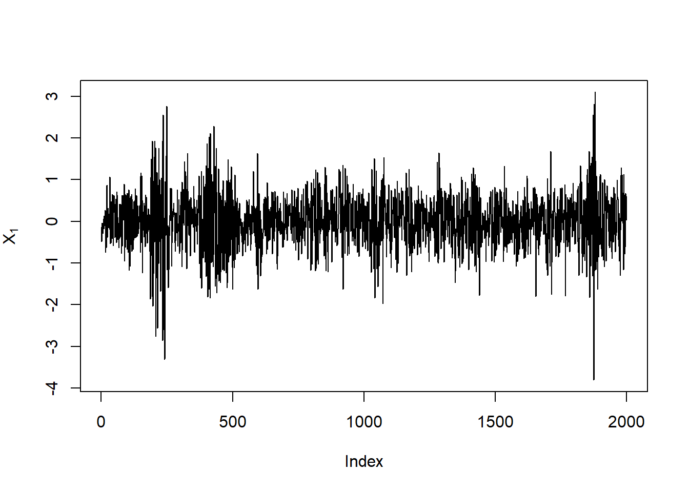
plot(X[,2], type = "l", ylab = expression(X[2]))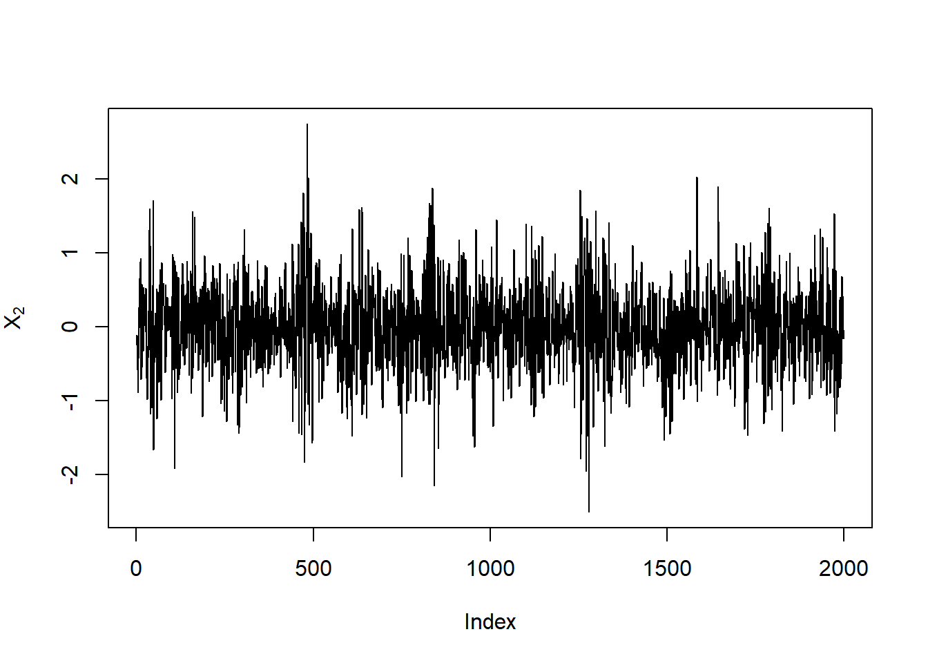
Plot the corresponding volatilities (\(\sigma_t\)):
plot(sig[,1], type = "h", ylab = expression(sigma[1]))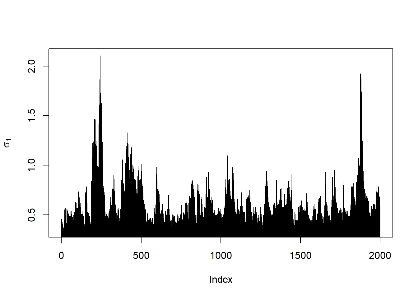
plot(sig[,2], type = "h", ylab = expression(sigma[2]))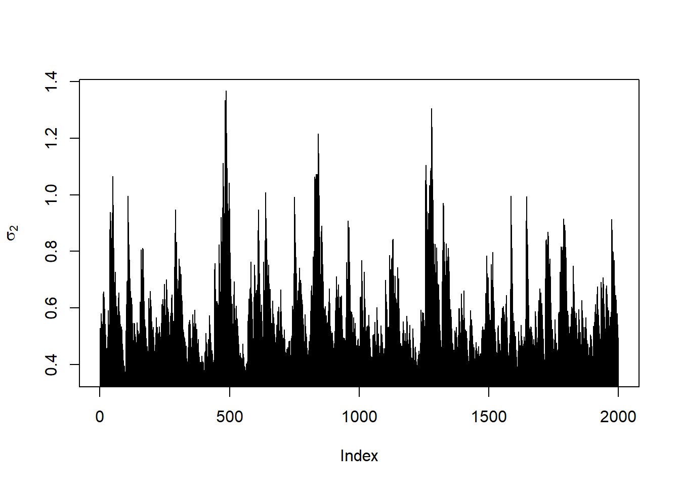
Plot the corresponding unstandardized residuals (\(\varepsilon_t\)):
plot(eps[,1], type = "l", ylab = expression(epsilon[1]))
plot(eps[,2], type = "l", ylab = expression(epsilon[2]))
Compute the standardized residuals (\(Z_t\)):
Z = eps/sig
plot(Z[,1], type = "p", ylab = expression(Z[1]))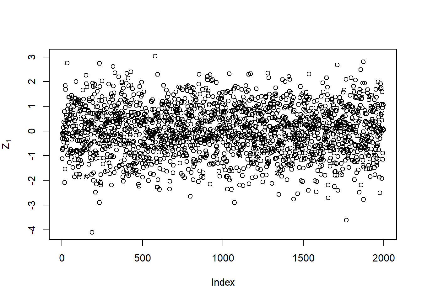
plot(Z[,2], type = "p", ylab = expression(Z[2]))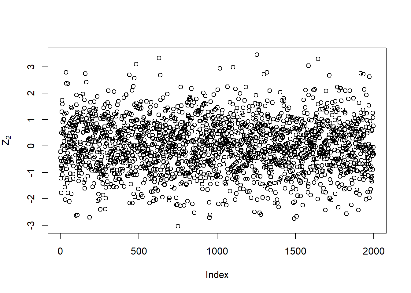
## Check their N(0,1) distribution
qq_plot(Z[,1])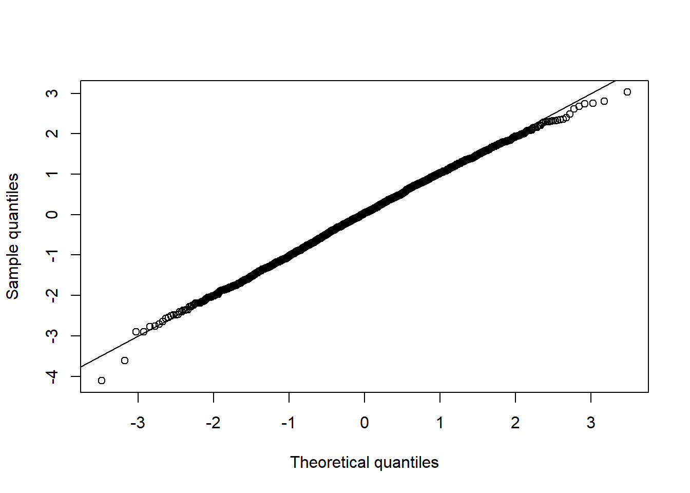
qq_plot(Z[,2])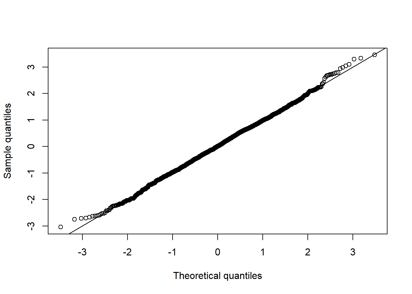
## Check their joint distribution
plot(Z, xlab = expression(Z[1]), ylab = expression(Z[2]))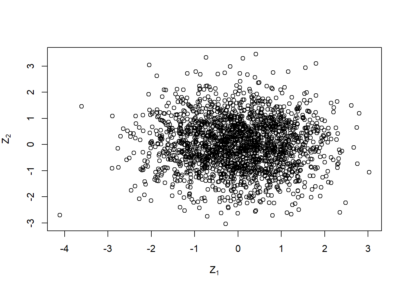
## Note: By doing all of this backwards, one can put different joint distributions
##       on the standard residuals. This will become clear after Chapters 6 and 7.
There are also special plotting functions for ‘uGARCHpath’ objects:
plot(paths, which = 1) # plots sig[,1] (no matter how many 'paths')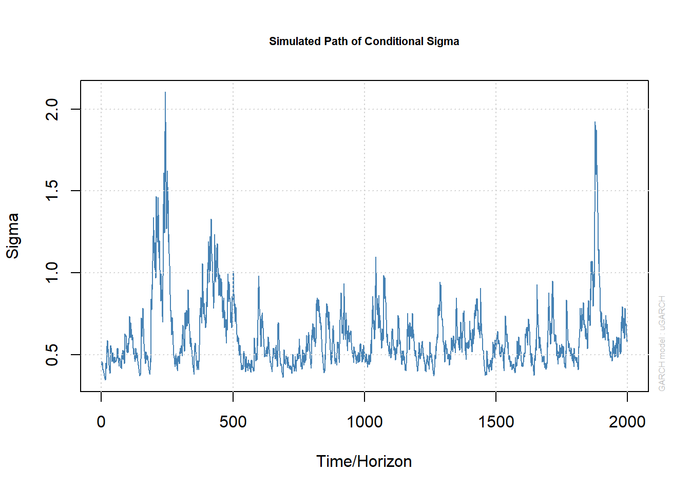
plot(paths, which = 2) # plots X[,1]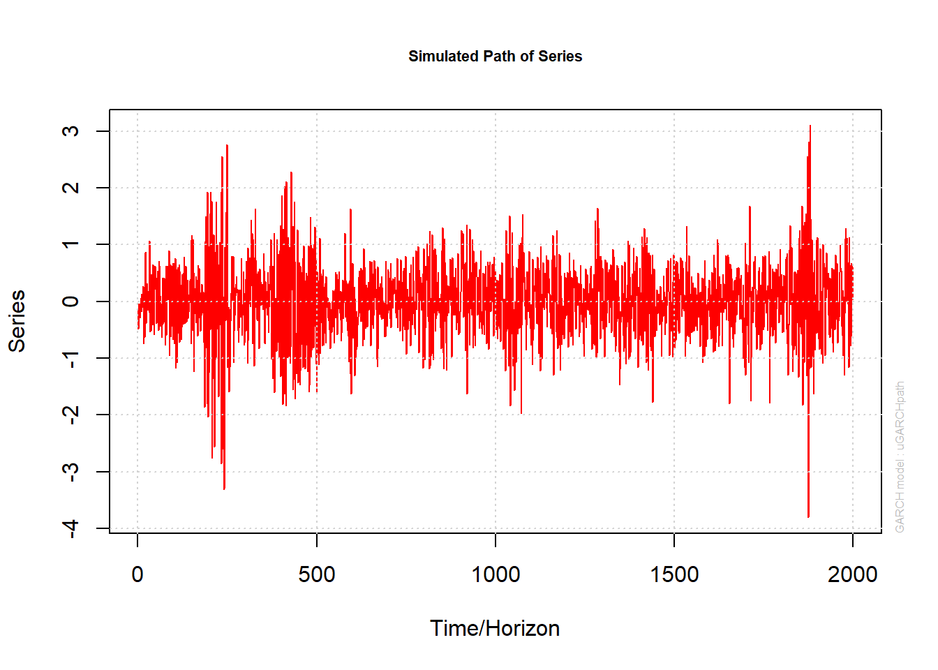
plot(paths, which = 3) # plots kernel density estimate of sig[,1]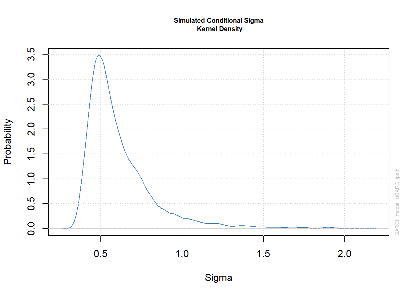
plot(paths, which = 4) # plots kernel density estimate of X[,1]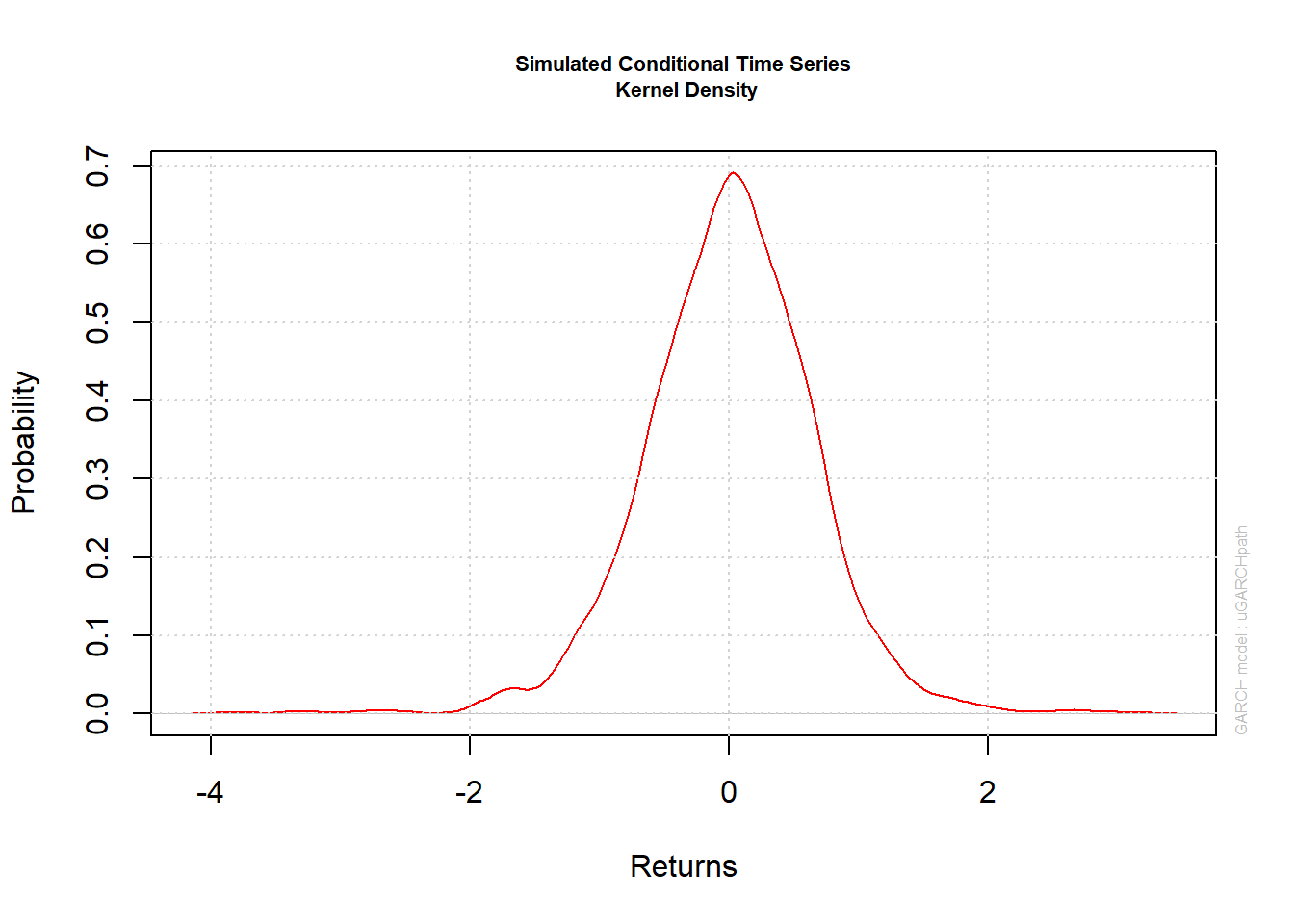
## How to see the documentation of the plot function
showMethods("plot")
## Function: plot (package base)
## x="ANY", y="ANY"
## x="Copula", y="ANY"
## x="density", y="missing"
## (inherited from: x="ANY", y="ANY")
## x="GPDFIT", y="missing"
## x="GPDTAILS", y="missing"
## x="matrix", y="missing"
## (inherited from: x="ANY", y="ANY")
## x="mvdc", y="ANY"
## x="numeric", y="missing"
## (inherited from: x="ANY", y="ANY")
## x="numeric", y="xts"
## (inherited from: x="ANY", y="ANY")
## x="profile.mle", y="missing"
## x="timeDate", y="ANY"
## x="timeSeries", y="ANY"
## x="uGARCHboot", y="missing"
## x="uGARCHdistribution", y="missing"
## x="uGARCHfilter", y="missing"
## x="uGARCHfit", y="missing"
## x="uGARCHforecast", y="missing"
## x="uGARCHpath", y="missing"
## x="uGARCHroll", y="missing"
## x="uGARCHsim", y="missing"getMethod("plot", signature = c(x = "uGARCHpath", y = "missing"))## Method Definition:
##
## function (x, y, ...)
## {
## .local <- function (x, which = "ask", m.sim = 1, ...)
## {
## choices = c("Conditional SD Simulation Path", "Return Series Simulation Path",
## "Conditional SD Simulation Density", "Return Series Simulation Path Density")
## .intergarchpathPlot(x, choices = choices, plotFUN = paste(".plot.garchpath",
## 1:4, sep = "."), which = which, m.sim = m.sim, ...)
## invisible(x)
## }
## .local(x, ...)
## }
## <bytecode: 0x0000000025d19918>
## <environment: namespace:rugarch>
##
## Signatures:
## x y
## target "uGARCHpath" "missing"
## defined "uGARCHpath" "missing"4.2.4 Does the simulated series conform to our univariate stylized facts?
We (only) consider the first path here:
acf(X[,1], main = expression(X[1])) # => no serial correlation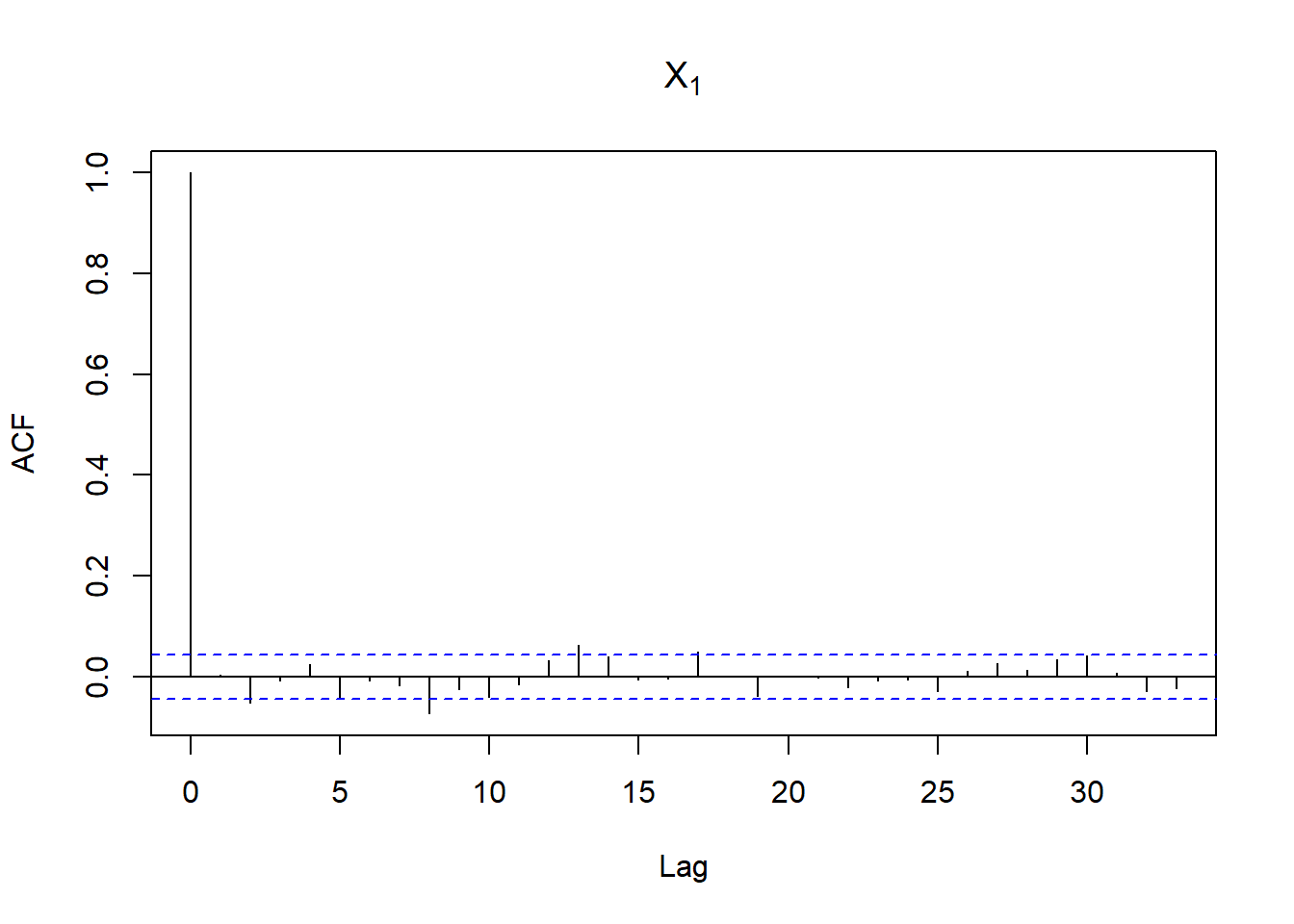
acf(abs(X[,1]), main = expression(group("|",X[1],"|"))) # => profound serial correlation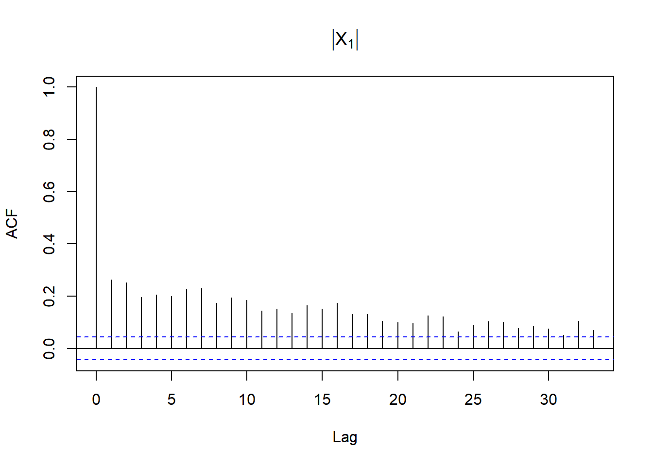
qq_plot(X[,1], method = "empirical", main = "Normal Q-Q plot") # => heavier tailed than normal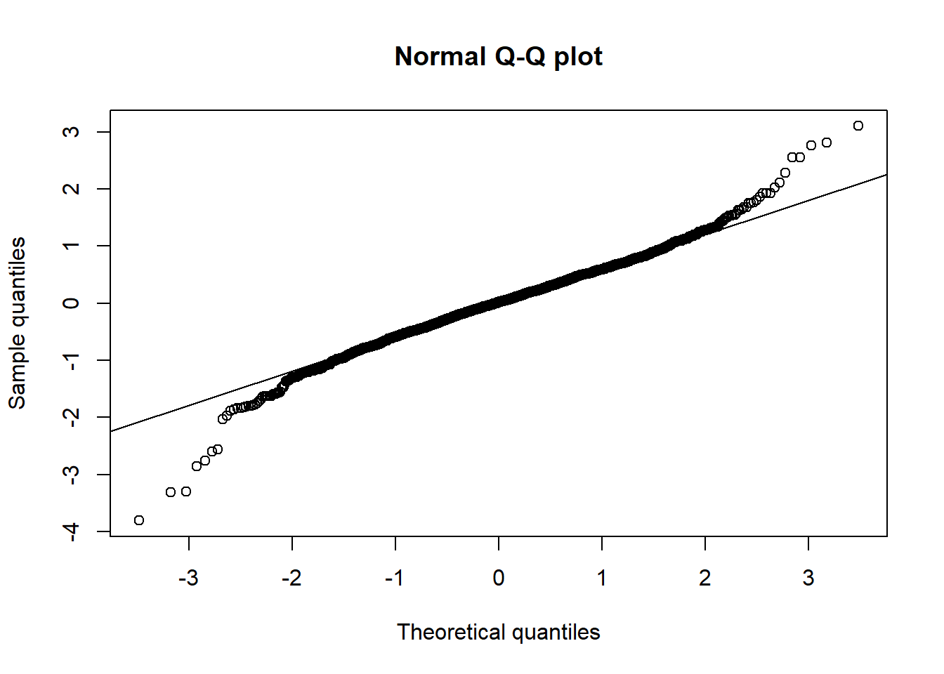
shapiro.test(X[,1]) # Normal rejected##
## Shapiro-Wilk normality test
##
## data: X[, 1]
## W = 0.98056685, p-value = 7.244413e-164.3 GARCH estimation
Estimation of univariate GARCH models
library(rugarch)
library(zoo)
library(ADGofTest) # for ad.test()
library(moments) # for skewness(), kurtosis()
library(qrmdata)
library(qrmtools)
4.3.1 S&P 500 data
Load S&P 500 data:
data("SP500")
plot.zoo(SP500, xlab = "Time")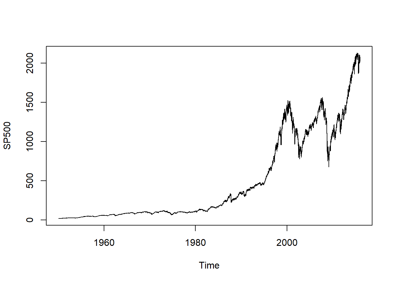
Extract the data we work with and build log-returns:
SPdata = SP500['2006-01-01/2009-12-31'] # 4 years of data
X = returns(SPdata)
plot.zoo(X, xlab = "Time")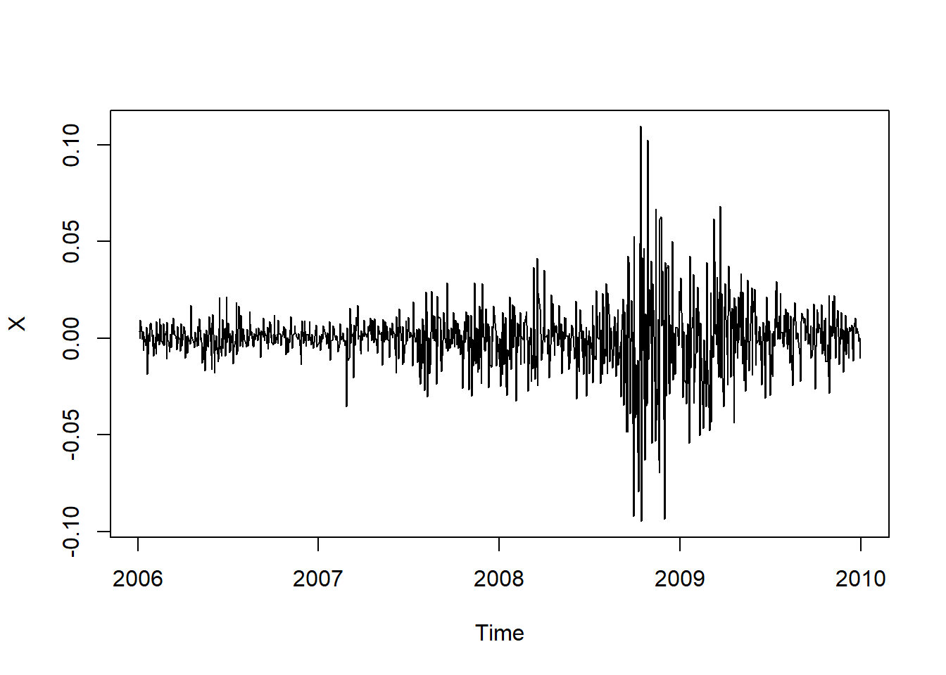
4.3.2 Fit an \(\text{AR}(1)\text{-}\text{GARCH}(1,1)\) model with normal innovations
Model specification (without fixed.pars, so without keeping any parameter fixed during the optimization):
uspec.N = ugarchspec(variance.model = list(model = "sGARCH", garchOrder = c(1,1)),
                      mean.model = list(armaOrder = c(1,0), # AR(1) part
                                        include.mean = TRUE), # with mean
                      distribution.model = "norm") # standard normal innovations
(fit.N = ugarchfit(spec = uspec.N, data = X))
##
## *---------------------------------*
## * GARCH Model Fit *
## *---------------------------------*
##
## Conditional Variance Dynamics
## -----------------------------------
## GARCH Model : sGARCH(1,1)
## Mean Model : ARFIMA(1,0,0)
## Distribution : norm
##
## Optimal Parameters
## ------------------------------------
## Estimate Std. Error t value Pr(>|t|)
## mu 0.000454 0.000261 1.7384 0.08214
## ar1 -0.105319 0.034015 -3.0963 0.00196
## omega 0.000002 0.000001 1.1298 0.25857
## alpha1 0.089398 0.014545 6.1465 0.00000
## beta1 0.903541 0.013916 64.9295 0.00000
##
## Robust Standard Errors:
## Estimate Std. Error t value Pr(>|t|)
## mu 0.000454 0.000200 2.27194 0.023090
## ar1 -0.105319 0.026755 -3.93641 0.000083
## omega 0.000002 0.000011 0.14297 0.886310
## alpha1 0.089398 0.051905 1.72235 0.085007
## beta1 0.903541 0.065681 13.75643 0.000000
##
## LogLikelihood : 3052.050378
##
## Information Criteria
## ------------------------------------
##
## Akaike -6.0578
## Bayes -6.0333
## Shibata -6.0578
## Hannan-Quinn -6.0485
##
## Weighted Ljung-Box Test on Standardized Residuals
## ------------------------------------
## statistic p-value
## Lag[1] 0.04276 0.8362
## Lag[2*(p+q)+(p+q)-1][2] 0.86117 0.8195
## Lag[4*(p+q)+(p+q)-1][5] 1.57982 0.8267
## d.o.f=1
## H0 : No serial correlation
##
## Weighted Ljung-Box Test on Standardized Squared Residuals
## ------------------------------------
## statistic p-value
## Lag[1] 4.896 0.02692
## Lag[2*(p+q)+(p+q)-1][5] 5.511 0.11700
## Lag[4*(p+q)+(p+q)-1][9] 6.546 0.24029
## d.o.f=2
##
## Weighted ARCH LM Tests
## ------------------------------------
## Statistic Shape Scale P-Value
## ARCH Lag[3] 0.1787 0.500 2.000 0.6725
## ARCH Lag[5] 0.9852 1.440 1.667 0.7373
## ARCH Lag[7] 1.0955 2.315 1.543 0.8975
##
## Nyblom stability test
## ------------------------------------
## Joint Statistic: 18.5
## Individual Statistics:
## mu 0.09407
## ar1 0.21794
## omega 3.08931
## alpha1 0.32485
## beta1 0.27671
##
## Asymptotic Critical Values (10% 5% 1%)
## Joint Statistic: 1.28 1.47 1.88
## Individual Statistic: 0.35 0.47 0.75
##
## Sign Bias Test
## ------------------------------------
## t-value prob sig
## Sign Bias 0.627 0.5308
## Negative Sign Bias 0.977 0.3288
## Positive Sign Bias 1.506 0.1324
## Joint Effect 4.253 0.2354
##
##
## Adjusted Pearson Goodness-of-Fit Test:
## ------------------------------------
## group statistic p-value(g-1)
## 1 20 74.64 1.534e-08
## 2 30 89.75 3.984e-08
## 3 40 102.55 1.287e-07
## 4 50 111.89 7.998e-07
##
##
## Elapsed time : 0.1189601421## Note: Fit to 'X', not 'SPdata'!The fit contains a lot of information:
The parameter estimates are the “Optimal Parameters” (at the top)
plot(fit.N)will take us into a menu system (below are the most important ones)
Series with conditional quantiles:
plot(fit.N, which = 2)##
## please wait...calculating quantiles...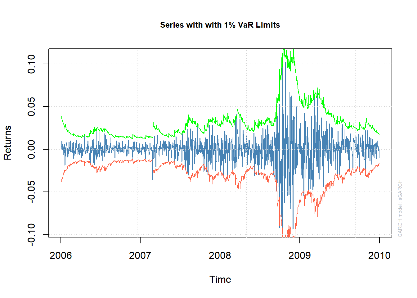
layout(matrix(1:4, ncol = 2, byrow = TRUE)) # specify (2,2)-matrix of plots
plot(fit.N, which = 6) # ACF of absolute data |X_t| (shows serial correlation)
plot(fit.N, which = 9) # Q-Q plot of standardized residuals Z_t (shows leptokurtosis of Z_t; normal assumption not supported)
plot(fit.N, which = 10) # ACF of standardized residuals Z_t (shows AR dynamics do a reasonable job of explaining conditional mean)
plot(fit.N, which = 11) # ACF of squared standardized residuals Z_t^2 (shows GARCH dynamics do a reasonable job of explaining conditional sd)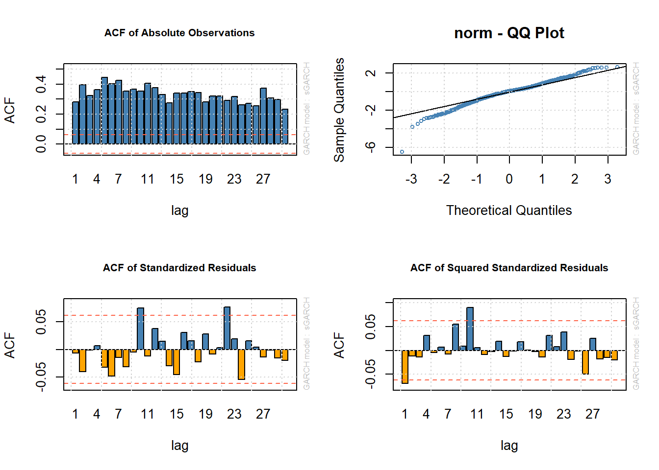
layout(1) # restore layout4.3.3 Fit an \(\text{AR}(1)\text{-}\text{GARCH}(1,1)\) model with Student \(t\) innovations
Now consider \(t\) innovations:
uspec.t = ugarchspec(variance.model = list(model = "sGARCH", garchOrder = c(1,1)),
                      mean.model = list(armaOrder = c(1,0), include.mean = TRUE),
                      distribution.model = "std") # standardized Student t innovations
(fit.t = ugarchfit(spec = uspec.t, data = X))
##
## *---------------------------------*
## * GARCH Model Fit *
## *---------------------------------*
##
## Conditional Variance Dynamics
## -----------------------------------
## GARCH Model : sGARCH(1,1)
## Mean Model : ARFIMA(1,0,0)
## Distribution : std
##
## Optimal Parameters
## ------------------------------------
## Estimate Std. Error t value Pr(>|t|)
## mu 0.000717 0.000238 3.00685 0.002640
## ar1 -0.080433 0.030491 -2.63792 0.008342
## omega 0.000001 0.000002 0.35601 0.721834
## alpha1 0.088331 0.025187 3.50705 0.000453
## beta1 0.910669 0.023094 39.43249 0.000000
## shape 5.676777 1.240099 4.57768 0.000005
##
## Robust Standard Errors:
## Estimate Std. Error t value Pr(>|t|)
## mu 0.000717 0.000167 4.285660 0.000018
## ar1 -0.080433 0.023078 -3.485262 0.000492
## omega 0.000001 0.000012 0.068722 0.945211
## alpha1 0.088331 0.110059 0.802578 0.422219
## beta1 0.910669 0.101817 8.944156 0.000000
## shape 5.676777 3.584508 1.583698 0.113263
##
## LogLikelihood : 3079.257193
##
## Information Criteria
## ------------------------------------
##
## Akaike -6.1099
## Bayes -6.0805
## Shibata -6.1099
## Hannan-Quinn -6.0987
##
## Weighted Ljung-Box Test on Standardized Residuals
## ------------------------------------
## statistic p-value
## Lag[1] 0.607 0.4359
## Lag[2*(p+q)+(p+q)-1][2] 1.399 0.4952
## Lag[4*(p+q)+(p+q)-1][5] 2.140 0.6706
## d.o.f=1
## H0 : No serial correlation
##
## Weighted Ljung-Box Test on Standardized Squared Residuals
## ------------------------------------
## statistic p-value
## Lag[1] 3.469 0.06251
## Lag[2*(p+q)+(p+q)-1][5] 3.941 0.26147
## Lag[4*(p+q)+(p+q)-1][9] 4.673 0.47891
## d.o.f=2
##
## Weighted ARCH LM Tests
## ------------------------------------
## Statistic Shape Scale P-Value
## ARCH Lag[3] 0.1607 0.500 2.000 0.6886
## ARCH Lag[5] 0.6916 1.440 1.667 0.8260
## ARCH Lag[7] 0.8583 2.315 1.543 0.9355
##
## Nyblom stability test
## ------------------------------------
## Joint Statistic: 75.3735
## Individual Statistics:
## mu 0.07419
## ar1 0.13886
## omega 22.91513
## alpha1 0.33557
## beta1 0.30392
## shape 0.60982
##
## Asymptotic Critical Values (10% 5% 1%)
## Joint Statistic: 1.49 1.68 2.12
## Individual Statistic: 0.35 0.47 0.75
##
## Sign Bias Test
## ------------------------------------
## t-value prob sig
## Sign Bias 0.5119 0.6088
## Negative Sign Bias 1.1340 0.2571
## Positive Sign Bias 1.6187 0.1058
## Joint Effect 4.6098 0.2027
##
##
## Adjusted Pearson Goodness-of-Fit Test:
## ------------------------------------
## group statistic p-value(g-1)
## 1 20 47.52 0.0003009
## 2 30 57.18 0.0013666
## 3 40 69.39 0.0019542
## 4 50 92.51 0.0001714
##
##
## Elapsed time : 0.1659948826## The pictures are similar, but the Q-Q plot looks "better"
layout(matrix(1:4, ncol = 2, byrow = TRUE)) # specify (2,2)-matrix of plots
plot(fit.t, which = 6) # ACF of |X_t|
plot(fit.t, which = 9) # Q-Q plot of Z_t against a normal
plot(fit.t, which = 10) # ACF of Z_t
plot(fit.t, which = 11) # ACF of Z_t^2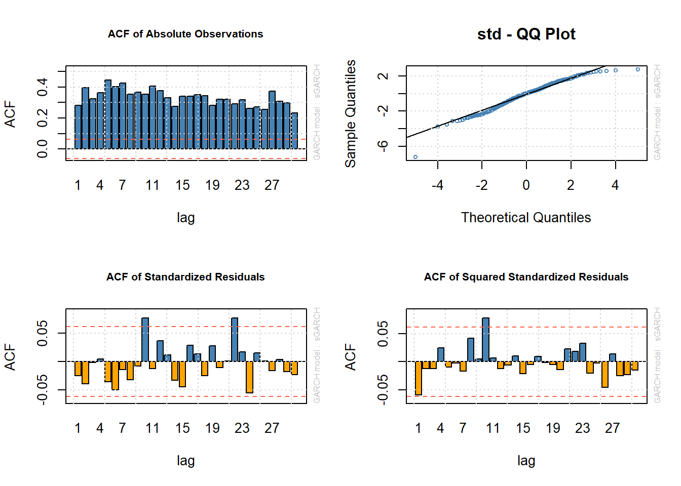
layout(1)4.3.4 Likelihood-ratio test for comparing the two models
The normal model is “nested within” the \(t\) model (appears from the \(t\) as special (limiting) case). The likelihood-ratio test tests:
\(H_0\): normal innovations are good enough
\(H_1\): \(t\) innovations necessary
Decision: We reject the null (in favor of the alternative) if the likelihood-ratio test statistic exceeds the 0.95 quantile of a chi-squared distribution with 1 degree of freedom (1 here as that’s the difference in the number of parameters for the two models)
The likelihood ratio statistic is twice the difference between the log-likelihoods:
LL.N = fit.N@fit$LLH # log-likelihood of the model based on normal innovations
LL.t = fit.t@fit$LLH # log-likelihood of the model based on t innovations
LRT = 2*(fit.t@fit$LLH-fit.N@fit$LLH) # likelihood-ratio test statistic
LRT > qchisq(0.95, 1) # => H0 is rejected
## [1] TRUE1-pchisq(LRT, df = 1) # p-value (probability of such an extreme result if normal hypothesis were true)## [1] 1.624256285e-134.3.5 Using Akaike’s information criterion to compare the two models
Akaike’s information criterion (AIC) can be used for model comparison.
Favor the model with smallest AIC.
Note: \(\text{AIC} = 2 \cdot \text{number of estimated parameters} - 2 \cdot \text{log-likelihood}\)
(AIC.N = 2*length(fit.N@fit$coef) - 2*LL.N)## [1] -6094.100756(AIC.t = 2*length(fit.t@fit$coef) - 2*LL.t)## [1] -6146.514386## => t model is preferred4.3.6 Exploring the structure of the fitted model object
Basic components:
class(fit.t)## [1] "uGARCHfit"
## attr(,"package")
## [1] "rugarch"getClass("uGARCHfit")## Class "uGARCHfit" [package "rugarch"]
##
## Slots:
##
## Name: fit model
## Class: vector vector
##
## Extends:
## Class "GARCHfit", directly
## Class "rGARCH", by class "GARCHfit", distance 2getSlots("uGARCHfit")## fit model
## "vector" "vector"fit.t.fit = fit.t@fit
names(fit.t.fit)## [1] "hessian" "cvar" "var" "sigma"
## [5] "condH" "z" "LLH" "log.likelihoods"
## [9] "residuals" "coef" "robust.cvar" "A"
## [13] "B" "scores" "se.coef" "tval"
## [17] "matcoef" "robust.se.coef" "robust.tval" "robust.matcoef"
## [21] "fitted.values" "convergence" "kappa" "persistence"
## [25] "timer" "ipars" "solver"fit.t.model = fit.t@model
names(fit.t.model)## [1] "modelinc" "modeldesc" "modeldata" "pars" "start.pars"
## [6] "fixed.pars" "maxOrder" "pos.matrix" "fmodel" "pidx"
## [11] "n.start"fit.t.model$modeldesc## $distribution
## [1] "std"
##
## $distno
## [1] 3
##
## $vmodel
## [1] "sGARCH"fit.t.model$pars## Level Fixed Include Estimate LB
## mu 7.165107918e-04 0 1 1 -1.283574006e-02
## ar1 -8.043335513e-02 0 1 1 -9.999999900e-01
## ma 0.000000000e+00 0 0 0 NA
## arfima 0.000000000e+00 0 0 0 NA
## archm 0.000000000e+00 0 0 0 NA
## mxreg 0.000000000e+00 0 0 0 NA
## omega 7.943575537e-07 0 1 1 2.220446049e-16
## alpha1 8.833096073e-02 0 1 1 0.000000000e+00
## beta1 9.106690144e-01 0 1 1 0.000000000e+00
## gamma 0.000000000e+00 0 0 0 NA
## eta1 0.000000000e+00 0 0 0 NA
## eta2 0.000000000e+00 0 0 0 NA
## delta 0.000000000e+00 0 0 0 NA
## lambda 0.000000000e+00 0 0 0 NA
## vxreg 0.000000000e+00 0 0 0 NA
## skew 0.000000000e+00 0 0 0 NA
## shape 5.676777036e+00 0 1 1 2.100000000e+00
## ghlambda 0.000000000e+00 0 0 0 NA
## xi 0.000000000e+00 0 0 0 NA
## UB
## mu 0.01283574006
## ar1 1.00000001000
## ma NA
## arfima NA
## archm NA
## mxreg NA
## omega 0.27724024905
## alpha1 0.99999999000
## beta1 0.99999999000
## gamma NA
## eta1 NA
## eta2 NA
## delta NA
## lambda NA
## vxreg NA
## skew NA
## shape 100.00000000000
## ghlambda NA
## xi NATo find out about extraction methods, see ?ugarchfit. Then follow a link to documentation for “uGARCHfit” object
Some extraction methods:
(param = coef(fit.t)) # estimated coefficients## mu ar1 omega alpha1
## 7.165107918e-04 -8.043335513e-02 7.943575537e-07 8.833096073e-02
## beta1 shape
## 9.106690144e-01 5.676777036e+00sig = sigma(fit.t) # estimated volatility
VaR.99 = quantile(fit.t, probs = 0.99) # estimated VaR at level 99%
Z = residuals(fit.t, standardize = TRUE) # estimated standardized residuals Z_tPlots:
plot.zoo(sig, xlab = "Time", ylab = expression(hat(sigma)[t]))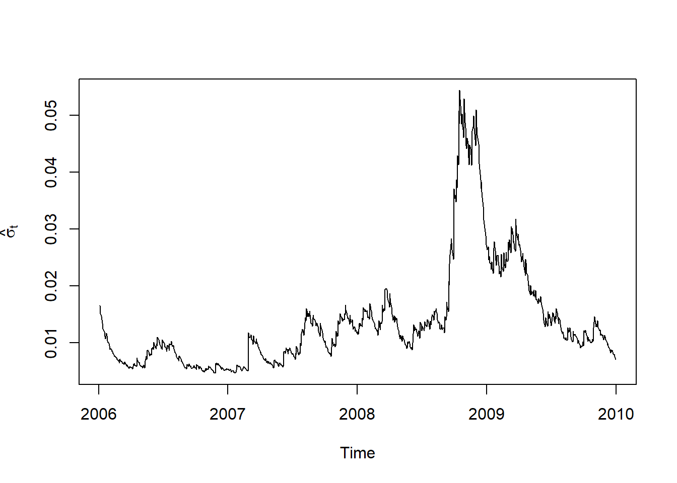
plot.zoo(VaR.99, xlab = "Time", ylab = expression(widehat(VaR)[0.99]))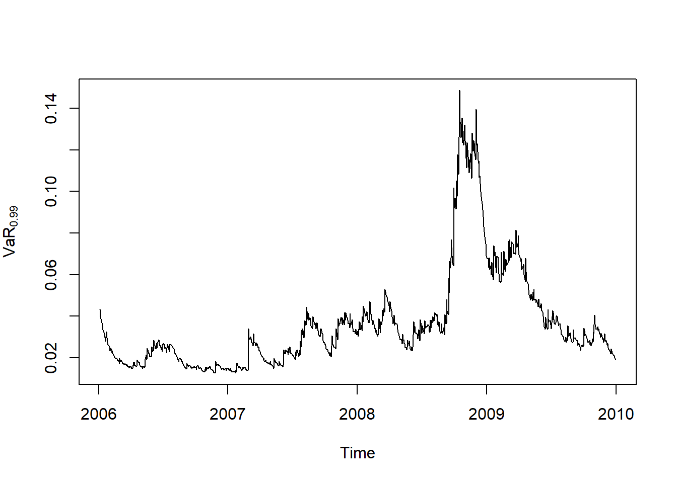
plot.zoo(Z, xlab = "Time", ylab = expression(hat(Z)[t]))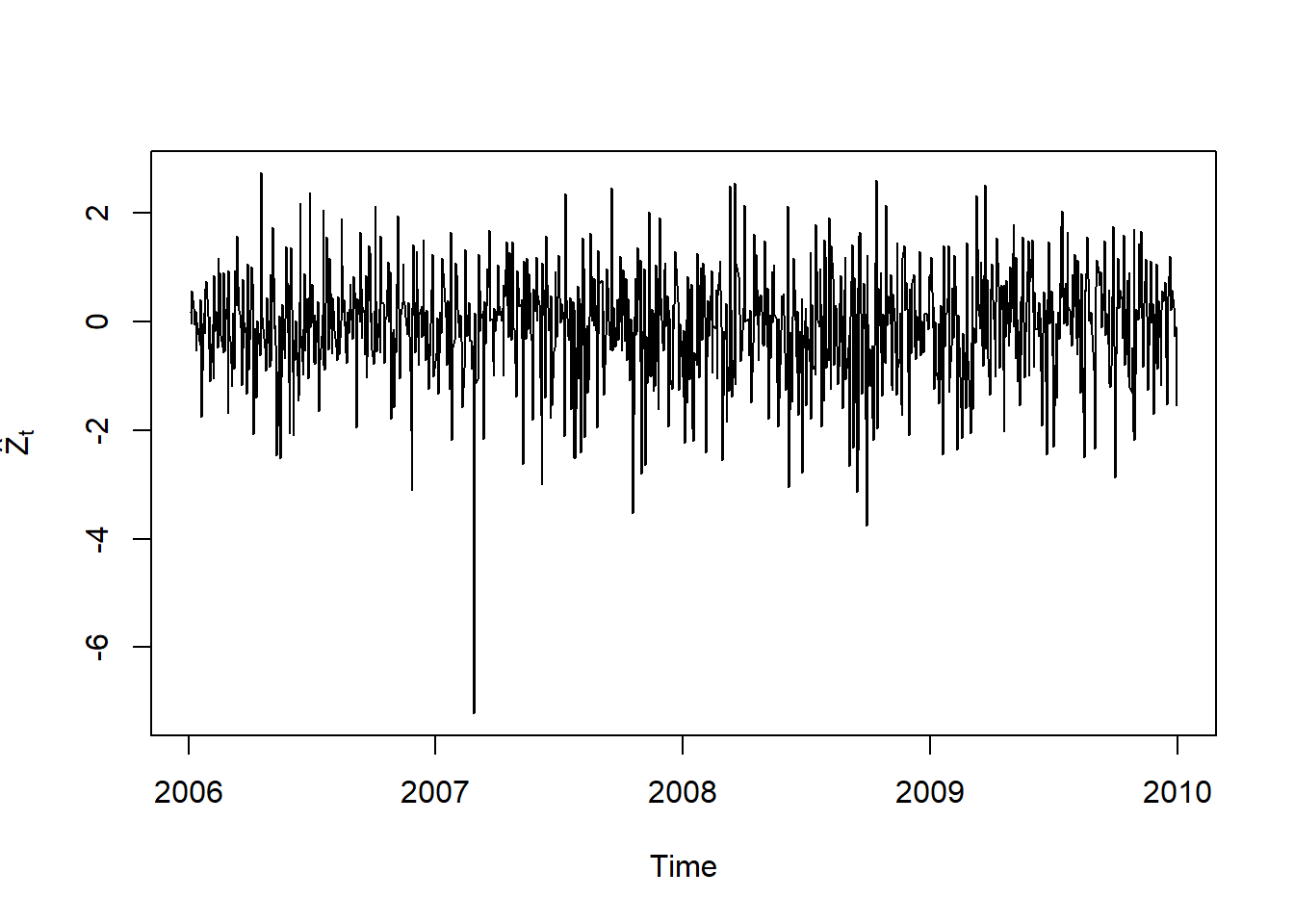
More residual checks:
(mu.Z = mean(Z)) # ok (should be ~= 0)## [1] -0.07232435396(sd.Z = as.vector(sd(Z))) # ok (should be ~= 1)## [1] 1.001556818skewness(Z) # should be 0 (is < 0 => left skewed)## X
## -0.6850474723hist(Z) # => left skewed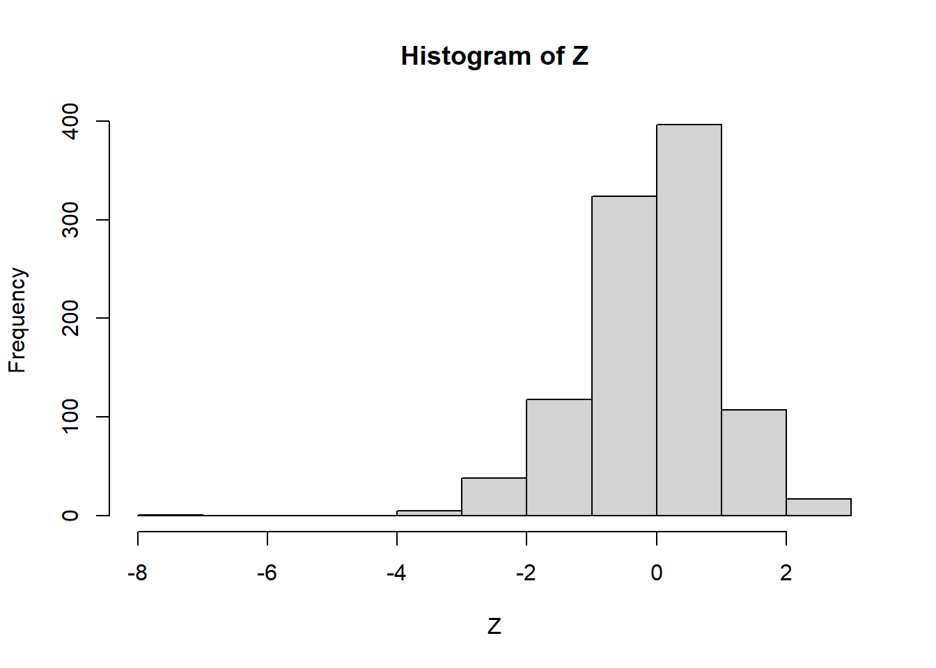
kurtosis(Z) # should be 6/(nu-4)## X
## 5.889080386nu = param[["shape"]] # estimated degrees-of-freedom
6/(nu-4) # => sample kurtosis larger than it should be## [1] 3.57829328pt.hat = function(q) pt((q-mu.Z)/sd.Z, df = nu) # estimated t distribution for Z
## Z ~ t_{hat(nu)}(hat(mu), hat(sig)^2) -> F_Z(z) = t_{hat(nu)}((z-hat(mu))/hat(sig))
ad.test(as.numeric(Z), distr.fun = pt.hat) # AD test##
## Anderson-Darling GoF Test
##
## data: as.numeric(Z) and pt.hat
## AD = 10.699031, p-value = 2.114166e-06
## alternative hypothesis: NA## => Anderson--Darling test rejects the estimated t distributionPossible things to try:
A GARCH model with asymmetric dynamics - GJR-GARCH
A GARCH model with asymmetric innovation distribution
Different ARMA specifications for the conditional mean
4.3.7 Forecasting/predicting from the fitted model
(forc = ugarchforecast(fit.t, n.ahead = 10))##
## *------------------------------------*
## * GARCH Model Forecast *
## *------------------------------------*
## Model: sGARCH
## Horizon: 10
## Roll Steps: 0
## Out of Sample: 0
##
## 0-roll forecast [T0=2009-12-31]:
## Series Sigma
## T+1 0.0015866 0.007513
## T+2 0.0006465 0.007562
## T+3 0.0007221 0.007611
## T+4 0.0007161 0.007659
## T+5 0.0007165 0.007707
## T+6 0.0007165 0.007754
## T+7 0.0007165 0.007802
## T+8 0.0007165 0.007848
## T+9 0.0007165 0.007895
## T+10 0.0007165 0.007941plot(forc, which = 1) # prediction of X_t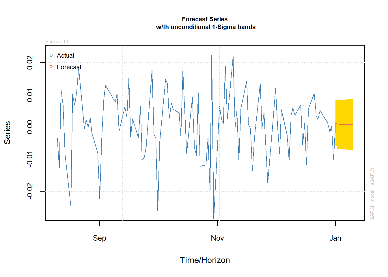
plot(forc, which = 3) # prediction of sigma_t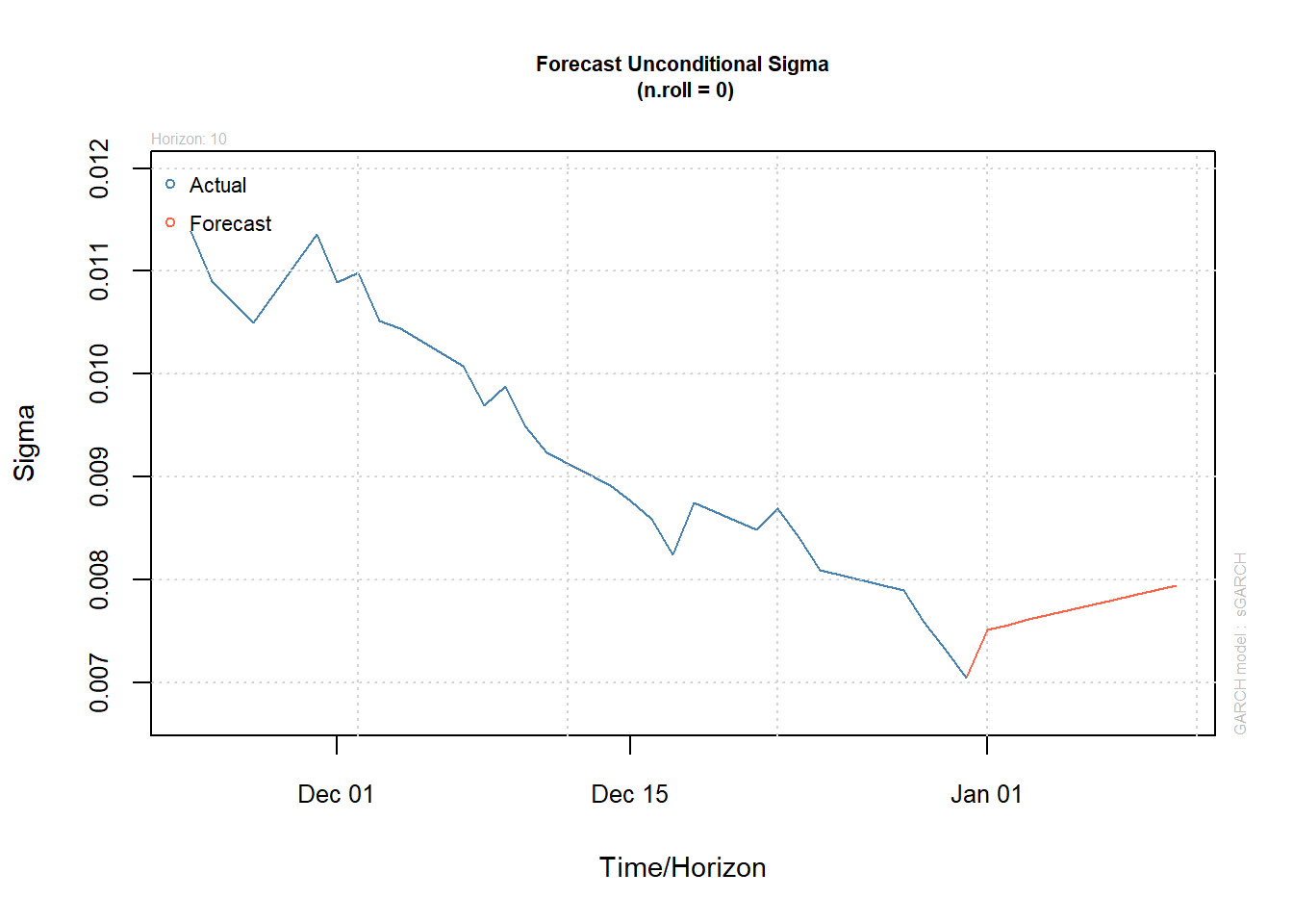
4.4 Simulate fit predict VaR under ARMA GARCH
Simulate an \(\text{ARMA}(1,1)\text{-}\text{GARCH}(1,1)\) process, fit such a process to the simulated data, estimate and backtest VaR, predict, simulate \(B\) paths, and compute corresponding VaR prediction with confidence intervals.
library(rugarch)
library(qrmtools)
4.4.1 Simulation
Model specification (for simulation):
armaOrder = c(1,1) # ARMA order
garchOrder = c(1,1) # GARCH order
nu = 3 # d.o.f. of the standardized distribution of Z_t
fixed.p = list(mu = 0, # our mu (intercept)
                ar1 = 0.5, # our phi_1 (AR(1) parameter of mu_t)
                ma1 = 0.3, # our theta_1 (MA(1) parameter of mu_t)
                omega = 4, # our alpha_0 (intercept)
                alpha1 = 0.4, # our alpha_1 (ARCH(1) parameter of sigma_t^2)
                beta1 = 0.2, # our beta_1 (GARCH(1) parameter of sigma_t^2)
                shape = nu) # d.o.f. nu for standardized t_nu innovations
varModel = list(model = "sGARCH", garchOrder = garchOrder)
spec = ugarchspec(varModel, mean.model = list(armaOrder = armaOrder),
                   fixed.pars = fixed.p, distribution.model = "std") # t standardized residuals
Simulate (\(X_t\)):
n = 1000 # sample size (= length of simulated paths)
x = ugarchpath(spec, n.sim = n, m.sim = 1, rseed = 271) # n.sim length of simulated path; m.sim = number of paths
## Note the difference:
## - ugarchpath(): simulate from a specified model
## - ugarchsim():  simulate from a fitted object
Extract the resulting series:
X = fitted(x) # simulated process X_t = mu_t + epsilon_t for epsilon_t = sigma_t * Z_t
sig = sigma(x) # volatilities sigma_t (conditional standard deviations)
eps = x@path$residSim # unstandardized residuals epsilon_t = sigma_t * Z_t
## Note: There are no extraction methods for the unstandardized residuals epsilon_t
Sanity checks (=> fitted() and sigma() grab out the right quantities):
stopifnot(all.equal(X,   x@path$seriesSim, check.attributes = FALSE),
          all.equal(sig, x@path$sigmaSim,  check.attributes = FALSE))
Plots:
plot(X, type = "l", xlab = "t", ylab = expression(X[t]))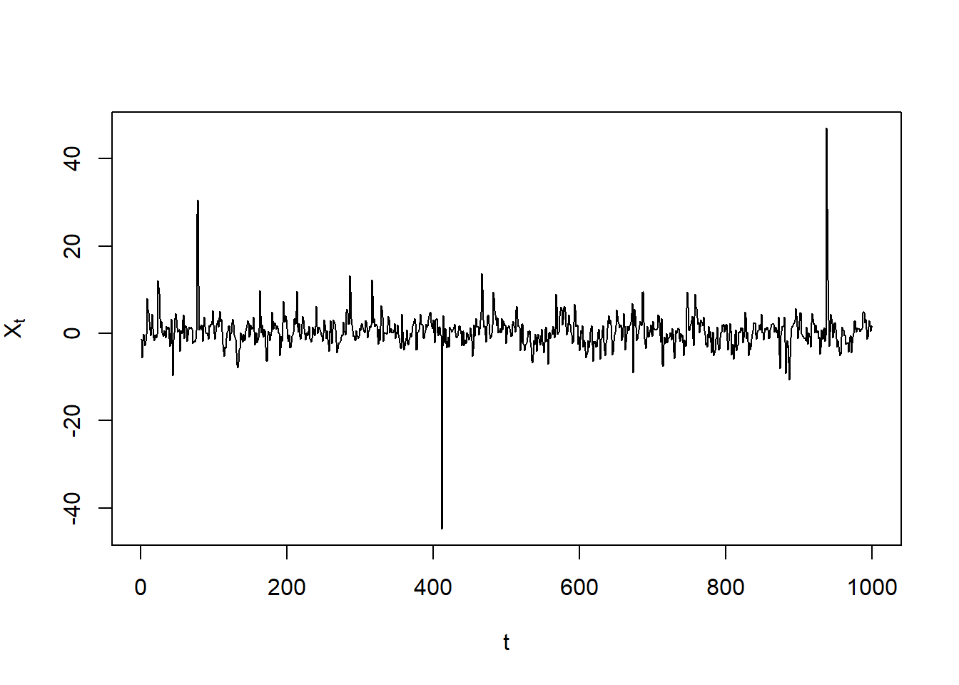
plot(sig, type = "h", xlab = "t", ylab = expression(sigma[t]))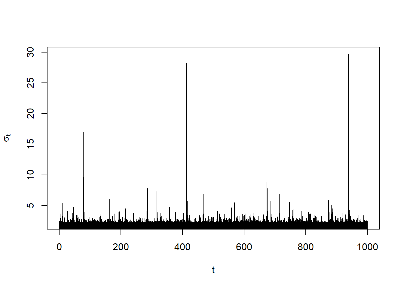
plot(eps, type = "l", xlab = "t", ylab = expression(epsilon[t]))
4.4.2 Fitting and checks
Now we do as if we don’t know the data-generating model. One would then normally fit models of various orders and decide which one to take. This step is omitted here for the sake of simplicity.
Fit an \(\text{ARMA}(1,1)\text{-}\text{GARCH}(1,1)\) model:
spec = ugarchspec(varModel, mean.model = list(armaOrder = armaOrder),
                   distribution.model = "std") # without fixed parameters here
fit = ugarchfit(spec, data = X) # fit
Extract the resulting seriesd:
mu. = fitted(fit) # fitted hat{mu}_t (= hat{X}_t)
sig. = sigma(fit) # fitted hat{sigma}_t
Sanity checks (=> fitted() and sigma() grab out the right quantities):
stopifnot(all.equal(as.numeric(mu.),  fit@fit$fitted.values),
          all.equal(as.numeric(sig.), fit@fit$sigma))
Plot data \(X_t\) and fitted \(\hat{\mu}_t\)
plot(X, type = "l", xlab = "t",
     ylab = expression("Data"~X[t]~"and fitted values"~hat(mu)[t]))
lines(as.numeric(mu.), col = adjustcolor("blue", alpha.f = 0.5))
legend("bottomright", bty = "n", lty = c(1,1),
       col = c("black", adjustcolor("blue", alpha.f = 0.5)),
       legend = c(expression(X[t]), expression(hat(mu)[t])))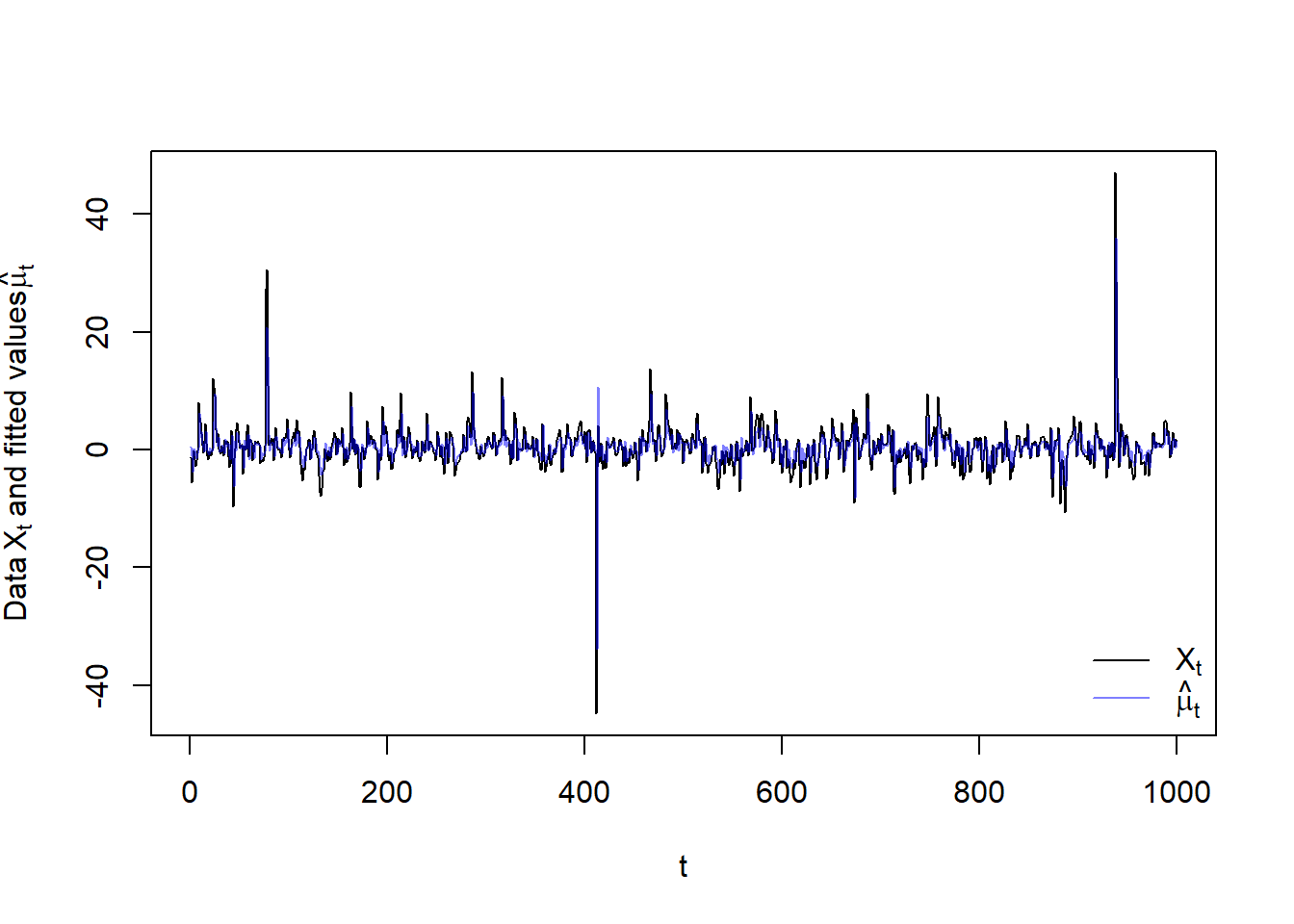
Plot the unstandardized residuals \(\varepsilon_t\):
resi = as.numeric(residuals(fit))
stopifnot(all.equal(fit@fit$residuals, resi))
plot(resi, type = "l", xlab = "t", ylab = expression(epsilon[t])) # check residuals epsilon_t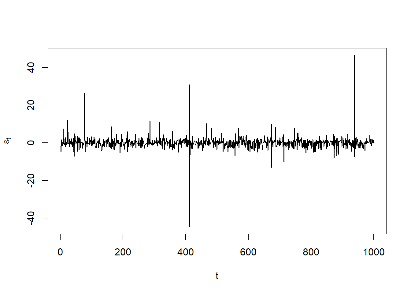
Q-Q plot of the standardized residuals \(Z_t\) against their specified \(t\) (\(t_\nu\) with variance \(1\)); as we generated the data, we know the exact \(t\) innovation distribution:
Z = fit@fit$z
stopifnot(all.equal(Z, as.numeric(resi/sig.)))
qq_plot(Z, FUN = function(p) sqrt((nu-2)/nu) * qt(p, df = nu),
        main = substitute("Q-Q plot of ("*Z[t]*") against the (here: correct) standardized"~
                              t[nu.], list(nu. = nu)))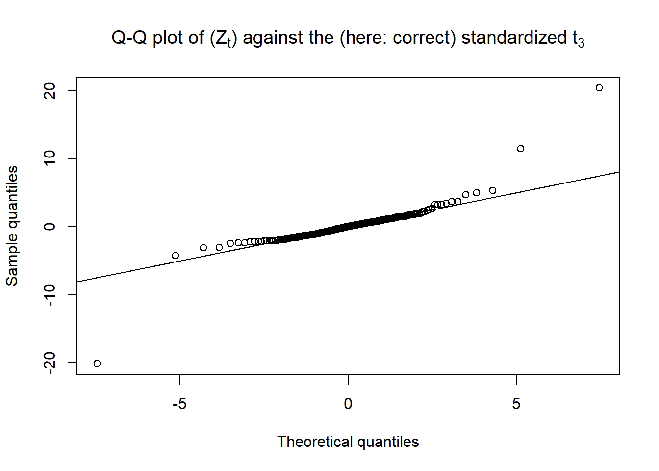
4.4.3 VaR estimates, checks and backtest
VaR confidence level we consider here:
alpha = 0.99Compute \(\text{VaR}_\alpha\) based on fitted \(\mu_t\) and \(\sigma_t\)
VaR. = as.numeric(quantile(fit, probs = alpha))
## Build manually and compare the two
nu. = fit@fit$coef["shape"] # extract (fitted) d.o.f. nu
VaR.. = as.numeric(mu. + sig. * sqrt((nu.-2)/nu.) * qt(alpha, df = nu.)) # VaR_alpha computed manually
stopifnot(all.equal(VaR.., VaR.))
## => quantile(<rugarch object>, probs = alpha) provides VaR_alpha = hat{mu}_t + hat{sigma}_t * q_Z(alpha)
4.4.4 Backtest VaR estimates
## Note: VaRTest() is written for the lower tail (not sign-adjusted losses)
##       (hence the complicated call here, requiring to refit the process to -X)
btest = VaRTest(1-alpha, actual = -X,
                 VaR = quantile(ugarchfit(spec, data = -X), probs = 1-alpha))
btest$expected.exceed # number of expected exceedances = (1-alpha) * n
## [1] 10btest$actual.exceed # actual exceedances## [1] 12## Unconditional test
btest$uc.H0 # corresponding null hypothesis## [1] "Correct Exceedances"btest$uc.Decision # test decision## [1] "Fail to Reject H0"## Conditional test
btest$cc.H0 # corresponding null hypothesis## [1] "Correct Exceedances & Independent"btest$cc.Decision # test decision## [1] "Fail to Reject H0"4.4.5 Predict (\(X_t\)) and \(\text{VaR}_\alpha\)
Predict from the fitted process:
fspec = getspec(fit) # specification of the fitted process
setfixed(fspec) = as.list(coef(fit)) # set the parameters to the fitted ones
m = ceiling(n / 10) # number of steps to forecast (roll/iterate m-1 times forward with frequency 1)
pred = ugarchforecast(fspec, data = X, n.ahead = 1, n.roll = m-1, out.sample = m) # predict from the fitted process
Extract the resulting series:
mu.predict = fitted(pred) # extract predicted X_t (= conditional mean mu_t; note: E[Z] = 0)
sig.predict = sigma(pred) # extract predicted sigma_t
VaR.predict = as.numeric(quantile(pred, probs = alpha)) # corresponding predicted VaR_alpha
Sanity checks:
stopifnot(all.equal(mu.predict, pred@forecast$seriesFor, check.attributes = FALSE),
          all.equal(sig.predict, pred@forecast$sigmaFor, check.attributes = FALSE)) # sanity check
Build predicted \(\text{VaR}_\alpha\) manually and compare the two:
VaR.predict. = as.numeric(mu.predict + sig.predict * sqrt((nu.-2)/nu.) *
                           qt(alpha, df = nu.)) # VaR_alpha computed manually
stopifnot(all.equal(VaR.predict., VaR.predict))
4.4.6 Simulate \(B\) paths from the fitted model
Simulate \(B\) paths:
B = 1000
set.seed(271)
X.sim.obj = ugarchpath(fspec, n.sim = m, m.sim = B) # simulate future paths
Compute simulated \(\text{VaR}_\alpha\) and corresponding (simulated) confidence intervals:
## Note: Each series is now an (m, B) matrix (each column is one path of length m)
X.sim = fitted(X.sim.obj) # extract simulated X_t
sig.sim = sigma(X.sim.obj) # extract sigma_t
eps.sim = X.sim.obj@path$residSim # extract epsilon_t
VaR.sim = (X.sim - eps.sim) + sig.sim * sqrt((nu.-2)/nu.) * qt(alpha, df = nu.) # (m, B) matrix
VaR.CI = apply(VaR.sim, 1, function(x) quantile(x, probs = c(0.025, 0.975)))
4.4.7 Plot
yran = range(X, # simulated path
              mu., VaR., # fitted conditional mean and VaR_alpha
              mu.predict, VaR.predict, VaR.CI) # predicted mean, VaR and CIs
myran = max(abs(yran))
yran = c(-myran, myran) # y-range for the plot
xran = c(1, length(X) + m) # x-range for the plot

## Simulated (original) data (X_t), fitted conditional mean mu_t and VaR_alpha
plot(X, type = "l", xlim = xran, ylim = yran, xlab = "Time t", ylab = "",
     main = "Simulated ARMA-GARCH, fit, VaR, VaR predictions and CIs")
lines(as.numeric(mu.), col = adjustcolor("darkblue", alpha.f = 0.5)) # hat{\mu}_t
lines(VaR., col = "darkred") # estimated VaR_alpha
mtext(paste0("Expected exceed.: ",btest$expected.exceed,"   ",
             "Actual exceed.: ",btest$actual.exceed,"   ",
             "Test: ", btest$cc.Decision),
      side = 4, adj = 0, line = 0.5, cex = 0.9) # label

## Predictions
t. = length(X) + seq_len(m) # future time points
lines(t., mu.predict, col = "blue") # predicted process X_t (or mu_t)
lines(t., VaR.predict, col = "red") # predicted VaR_alpha
lines(t., VaR.CI[1,], col = "orange") # lower 95%-CI for VaR_alpha
lines(t., VaR.CI[2,], col = "orange") # upper 95%-CI for VaR_alpha
legend("bottomright", bty = "n", lty = rep(1, 6), lwd = 1.6,
       col = c("black", adjustcolor("darkblue", alpha.f = 0.5), "blue",
               "darkred", "red", "orange"),
       legend = c(expression(X[t]), expression(hat(mu)[t]),
                  expression("Predicted"~mu[t]~"(or"~X[t]*")"),
                  substitute(widehat(VaR)[a], list(a = alpha)),
                  substitute("Predicted"~VaR[a], list(a = alpha)),
                  substitute("Simulated 95%-CI for"~VaR[a], list(a = alpha))))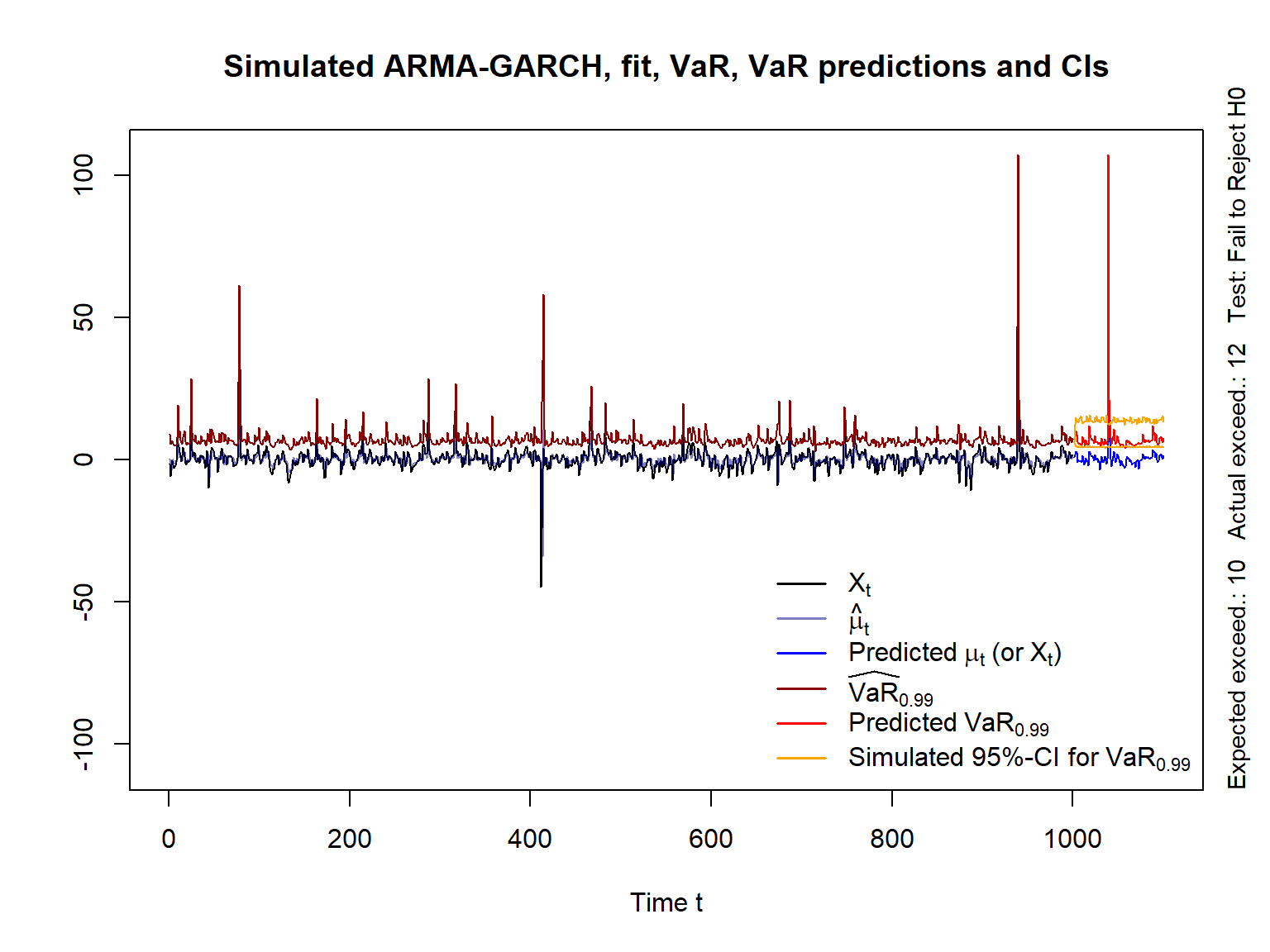
4.5 Exercises
library(xts)
library(rugarch)
library(qrmdata)
library(qrmtools)
options(digits = 10)
Exercise 4.1 (Fitting GARCH models to equity index return data) Take the set of closing prices of the S&P 500 index from 2006 to 2009 including the financial crisis; see the dataset SP500 of the R package qrmdata.
Fit \(\text{GARCH}(1, 1)\) models with standard normal, standardized \(t\) and standardized skewed \(t\) innovations to the negative log-returns; see the functions
ugarchspec()andugarchfit()in the R packagerugarch. Plot the resulting standardized residuals and Q-Q plots against the fitted innovation distributions.Add \(\text{AR}(1)\), \(\text{MA}(1)\) and \(\text{ARMA}(1, 1)\) models for the conditional mean and investigate whether this improves the resulting fit of the models.
Use your favourite model to calculate an in-sample estimate of volatility and an in-sample estimate of the 99% value-at-risk for the period.
## Data preparation
data(SP500)
S = SP500['2006-01-01/2019-12-31'] # pick out the data we work with
X.d = -returns(S)
## a)##' @title Scatterplot and Q-Q Plot of the Residuals for GARCH(1,1) Model Fit Assessment
##' @param x data
##' @param armaOrder ARMA (p,q) order
##' @param distribution.model innovation distribution (standardized)
##' @return fitted ARMA-GARCH(1,1) object (invisibly)
##' @author Marius Hofert
GARCH11_check = function(x, armaOrder, distribution.model = c("norm", "std", "sstd"))
{
## Check
distribution.model = match.arg(distribution.model)
## Model fit
uspec = ugarchspec(variance.model = list(model = "sGARCH", garchOrder = c(1, 1)),
mean.model = list(armaOrder = armaOrder, include.mean = TRUE),
distribution.model = distribution.model)
fit = ugarchfit(spec = uspec, data = x) # fit
resi = as.numeric(residuals(fit, standardize = TRUE)) # standardized residuals (equivalent to fit@fit$z)
## Quantile function of fitted innovation distribution
switch(distribution.model,
"norm" = {
qF = function(p) qdist("norm", p = p)
lab = c(distr = "Standard normal", info = NA)
},
"std" = {
nu = coef(fit)[["shape"]] # fitted degrees of freedom
qF = function(p) qdist("std", p = p, shape = nu)
## Note: As ./src/distributions.c -> qstd() reveals, this t distribution
## is already standardized to have variance 1 (so t_nu(0, (nu-2)/nu))
## when sigma = 1 (the default).
lab = c(distr = "Standardized t",
info = paste("Fitted degrees of freedom:", round(nu, 2)))
},
"sstd" = {
sk = coef(fit)[["skew"]] # fitted skewness parameter
nu = coef(fit)[["shape"]] # fitted degrees of freedom
qF = function(p) qdist("sstd", p = p, skew = sk, shape = nu)
## Note: Also this (skewed t) distribution is already standardized.
## This can also be quickly verified via:
## set.seed(271); var(rdist("sstd", n = 1e6, skew = 3.5, shape = 5.5))
lab = c(distr = "Standardized skewed t",
info = paste0("Fitted skewness: ",round(sk, 2),
"; fitted degrees of freedom: ",round(nu, 2)))
},
stop("Wrong 'distribution.model'"))
## Plots
layout(t(1:2))
plot(resi, ylab = paste("Residuals of GARCH(1,1) with",
tolower(lab["distr"]), "innovations")) # Scatterplot
mtext(lab["info"], side = 4, adj = 0, line = 0.5)
qq_plot(resi, FUN = qF, xlab = paste(lab["distr"], "quantiles")) # Q-Q plot
mtext(lab["info"], side = 4, adj = 0, line = 0.5)
layout(1)
invisible(fit)
}## Pure GARCH(1,1)GARCH11_check(X.d, armaOrder = c(0, 0), distribution.model = "norm") # standard normal innovations
GARCH11_check(X.d, armaOrder = c(0, 0), distribution.model = "std") # standardized t innovations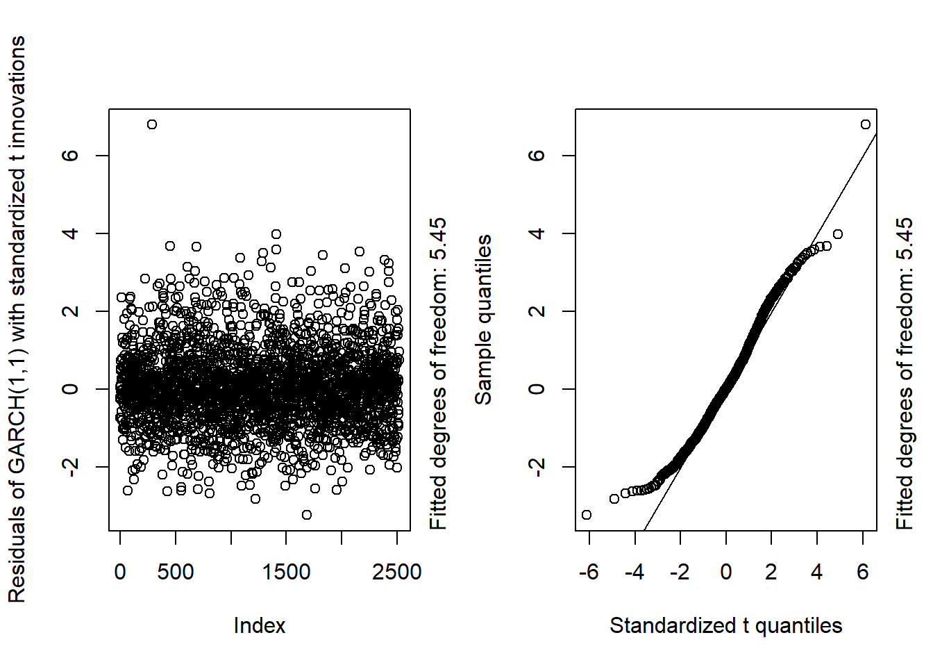
GARCH11_check(X.d, armaOrder = c(0, 0), distribution.model = "sstd") # standardized skewed t innovations
## By a small margin, the best seem to be the standardized skewed t distribution as
## innovation distribution.
## b)## AR(1)-GARCH(1,1)GARCH11_check(X.d, armaOrder = c(1, 0), distribution.model = "norm") # standard normal innovations
GARCH11_check(X.d, armaOrder = c(1, 0), distribution.model = "std") # standardized t innovations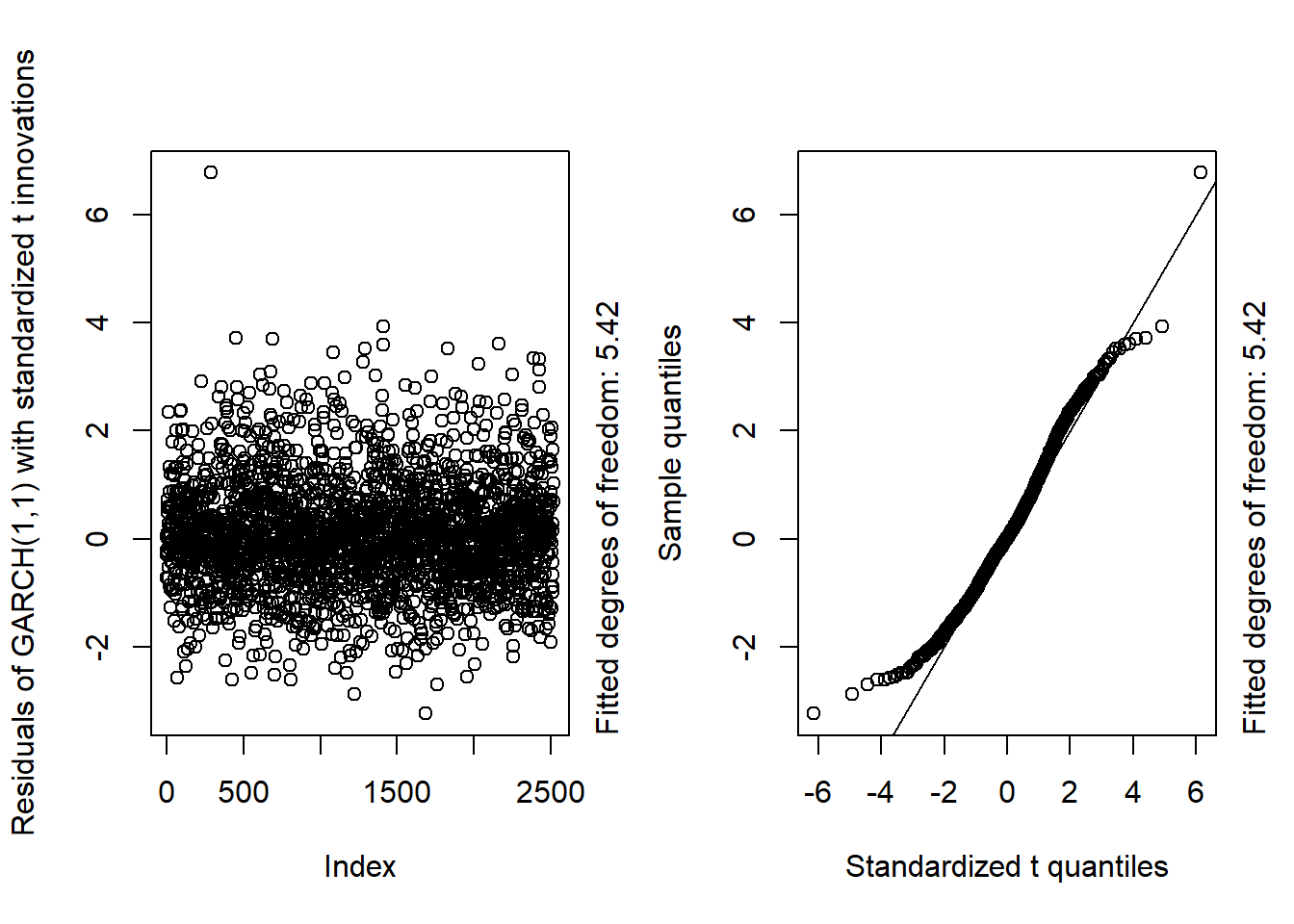
GARCH11_check(X.d, armaOrder = c(1, 0), distribution.model = "sstd") # standardized skewed t innovations
## MA(1)-GARCH(1,1)GARCH11_check(X.d, armaOrder = c(0, 1), distribution.model = "norm") # standard normal innovations
GARCH11_check(X.d, armaOrder = c(0, 1), distribution.model = "std") # standardized t innovations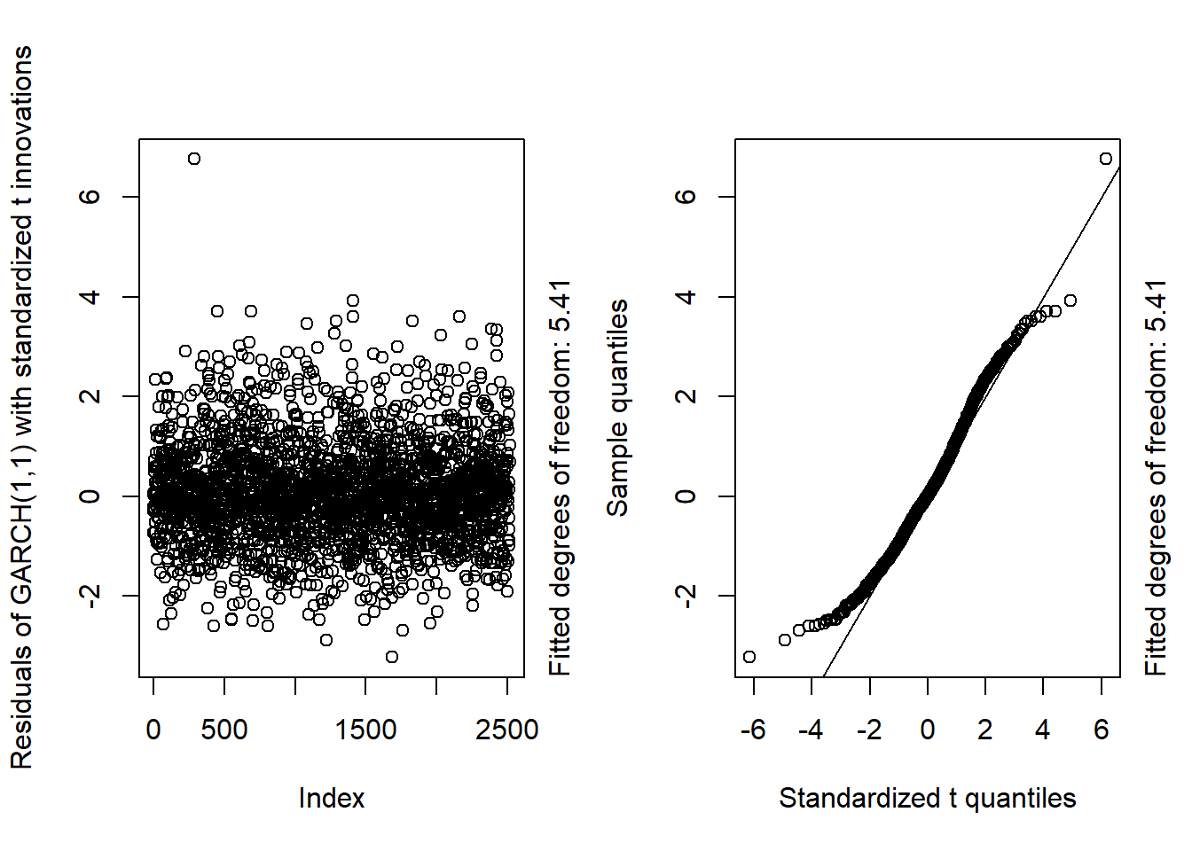
GARCH11_check(X.d, armaOrder = c(0, 1), distribution.model = "sstd") # standardized skewed t innovations
## ARMA(1,1)-GARCH(1,1)GARCH11_check(X.d, armaOrder = c(1, 1), distribution.model = "norm") # standard normal innovations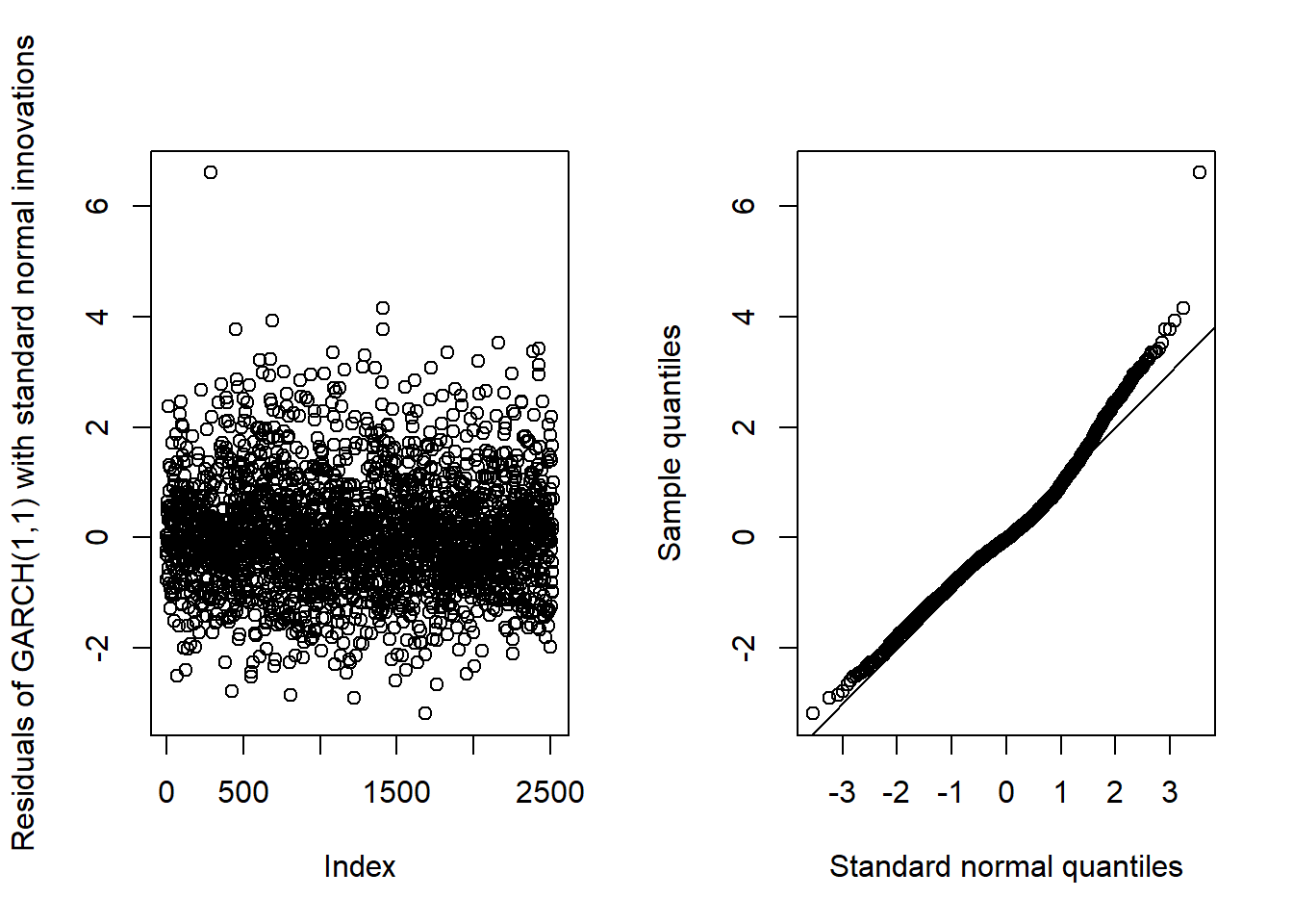
GARCH11_check(X.d, armaOrder = c(1, 1), distribution.model = "std") # standardized t innovations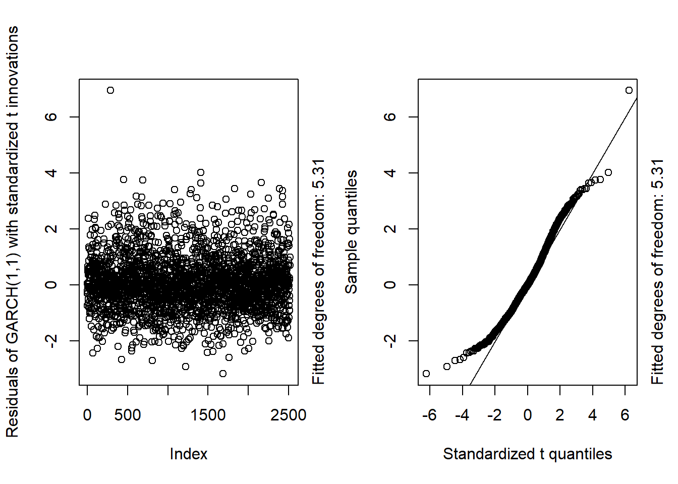
GARCH11_check(X.d, armaOrder = c(1, 1), distribution.model = "sstd") # standardized skewed t innovations
## Overall, we see that the resulting fit of the models cannot be improved by adding
## a low-order ARMA model for the conditional mean.
## c)## We work with the GARCH(1,1) model with skewed t innovations.
fit = GARCH11_check(X.d, armaOrder = c(0, 0), distribution.model = "sstd") # get fitted model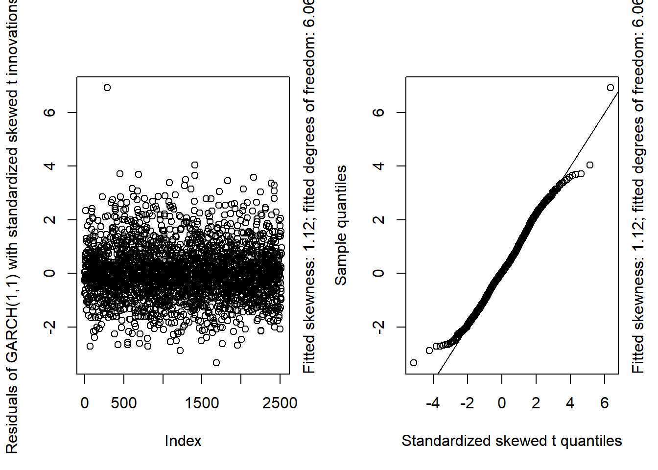
vola = sigma(fit) # = fit@fit$sigma = sqrt(fit@fit$var); in-sample (sigma_t) estimate
alpha = 0.99 # confidence level
mu = fitted(fit) # fitted conditional mean (here: constant, as armaOrder = c(0, 0))
VaR = mu + vola * qdist("sstd", p = alpha, # in-sample VaR_alpha estimate
                         skew = coef(fit)[["skew"]], shape = coef(fit)[["shape"]]) # manually computed
VaR. = quantile(fit, probs = alpha) # via rugarch()'s quantile method
stopifnot(all.equal(VaR, VaR., check.attributes = FALSE)) # comparison