Chapter 9 Market Risk
9.1 Standard methods for market risk
Estimating the risk measures VaR and ES with standard methods based on (BMW, Siemens) data from 2000-01-03 to 2009-12-31.
library(nvmix) # for rNorm(), fitStudent(), rStudent()
library(xts) # for na.fill()
library(qrmdata) # for the data
library(qrmtools) # for the data analysis
9.1.1 Working with the (BMW, Siemens) data
Load the data:
data(EURSTX_const)
db <- EURSTX_const
str(db) # check the *str*ucture of 'db'
## An 'xts' object on 2000-01-03/2015-12-31 containing:
## Data: num [1:4174, 1:50] NA NA NA NA NA NA NA NA NA NA ...
## - attr(*, "dimnames")=List of 2
## ..$ : NULL
## ..$ : chr [1:50] "ABI.BR" "AI.PA" "AIR.PA" "ALV.DE" ...
## Indexed by objects of class: [Date] TZ: UTC
## xts Attributes:
## List of 2
## $ src : chr "yahoo"
## $ updated: POSIXct[1:1], format: "2016-01-03 03:53:56"Pick out the sub-database of stock prices we work with and fill gaps:
time <- c("2000-01-03", "2009-12-31")
S <- db[paste0(time, collapse = "/"), c("BMW.DE", "SIE.DE")] # pick out data (data.frame)
str(S)
## An 'xts' object on 2000-01-03/2009-12-31 containing:
## Data: num [1:2609, 1:2] 16.1 15.5 15.2 15.1 15.1 ...
## - attr(*, "dimnames")=List of 2
## ..$ : NULL
## ..$ : chr [1:2] "BMW.DE" "SIE.DE"
## Indexed by objects of class: [Date] TZ: UTC
## xts Attributes:
## List of 2
## $ src : chr "yahoo"
## $ updated: POSIXct[1:1], format: "2016-01-03 03:53:56"head(S) # show the beginning## BMW.DE SIE.DE
## 2000-01-03 16.110 72.4512
## 2000-01-04 15.460 69.5241
## 2000-01-05 15.154 67.1715
## 2000-01-06 15.105 66.3500
## 2000-01-07 15.077 69.0192
## 2000-01-10 15.678 73.1262tail(S) # show the end## BMW.DE SIE.DE
## 2009-12-24 NA NA
## 2009-12-25 NA NA
## 2009-12-28 27.200 48.8042
## 2009-12-29 27.414 48.6317
## 2009-12-30 27.200 48.1666
## 2009-12-31 NA NAS <- na.fill(S, fill = "extend") # fill NAs (see also NA_plot(S))
tail(S)## BMW.DE SIE.DE
## 2009-12-24 27.38266667 48.23413333
## 2009-12-25 27.29133333 48.51916667
## 2009-12-28 27.20000000 48.80420000
## 2009-12-29 27.41400000 48.63170000
## 2009-12-30 27.20000000 48.16660000
## 2009-12-31 27.20000000 48.16660000colnames(S) <- c("BMW", "SIE")Use scatter plots of each time series to check if anything is ‘suspicious’:
plot.zoo(S[,"BMW"], main = "BMW stock data",
         xlab = "Date t", ylab = expression(Stock~price~S[t]))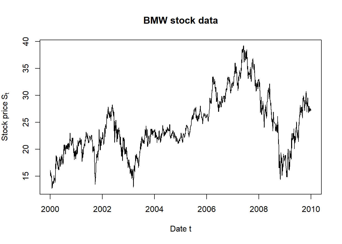
plot.zoo(S[,"SIE"], main = "SIEMENS stock data",
         xlab = "Date t", ylab = expression(Stock~price~S[t]))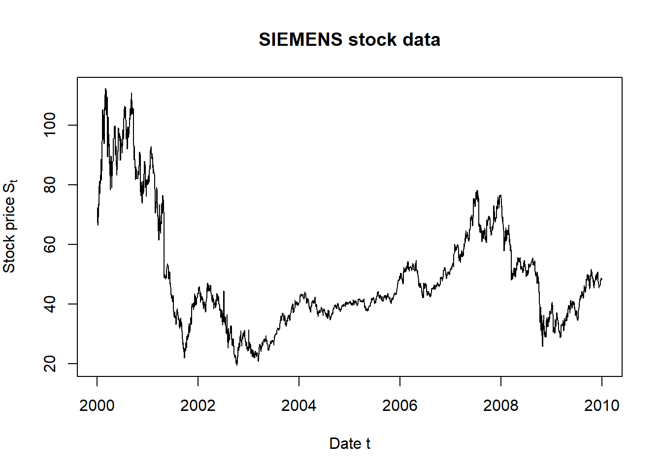
Compute the risk-factor changes and plot them (here: against each other):
X <- returns(S) # compute log-returns (sign-adjustment in loss operator below)
plot.zoo(X[,"BMW"], main = "BMW log-return data",
         xlab = "Date t", ylab = expression(Log-returns~X[t]))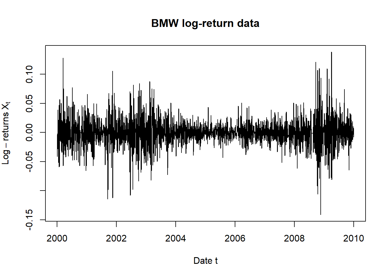
plot.zoo(X[,"SIE"], main = "SIE log-return data",
         xlab = "Date t", ylab = expression(Log-returns~X[t]))
X <- as.matrix(X)
plot(X, cex = 0.4)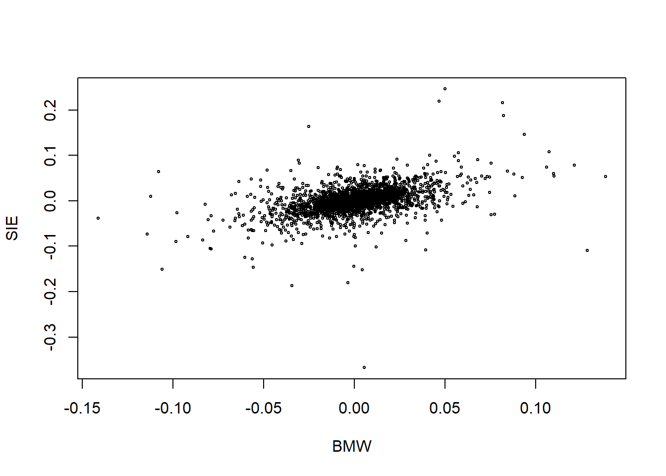
9.2 Implement (and document) some auxiliary functions
##' @title Compute the Loss Operator
##' @param x matrix of risk-factor changes
##' @param weights weights tilde{w}_{t,j} = lambda_j * S_{t,j}
##' @return losses -sum_{j=1}^d(tilde{w}_{t,j}(exp(X_{t+1,j})-1))
##' @author Marius Hofert
loss_operator <- function(x, weights)
    -rowSums(expm1(x) * matrix(weights, nrow = nrow(x), ncol = length(weights), byrow = TRUE))
##' @title Estimate VaR and ES
##' @param S stock data, an (n, d)-matrix
##' @param lambda number of shares of each stock
##' @param alpha confidence level for VaR and ES
##' @param method character string specifying the estimator
##' @param ... additional arguments passed to the various methods
##' @return list containing the estimated risk measures VaR and ES, and
##' possibly other results (depending on the estimator)
##' @author Marius Hofert
risk_measure <- function(S, lambda, alpha,
method = c("Var.Cov", "hist.sim", "MC.N", "MC.t", "POT"),
...)
{
## Input checks and conversions
if(!is.matrix(S)) S <- rbind(S, deparse.level = 0L) # guarantees that ncol() works
stopifnot(0 < alpha, alpha < 1, # check whether alpha is in (0,1)
length(lambda) == ncol(S), lambda > 0) # check length and sign of lambda
method <- match.arg(method) # match correct method if not fully provided
## Ingredients required for *all* methods
X <- returns(S) # compute risk-factor changes
if(!length(X)) stop("'S' should have more than just one line") # check
S. <- as.numeric(tail(S, n = 1)) # pick out last available stock prices ("today")
w. <- lambda * S. # weights tilde{w} today
## Method switch (now consider the various methods)
switch(method,
"Var.Cov" = { # variance-covariance method
## Estimate a multivariate normal distribution
mu.hat <- colMeans(X) # estimate the mean vector mu
Sigma.hat <- var(X) # estimate the covariance matrix Sigma
L.delta.mean <- -sum(w. * mu.hat) # mean of the approx. normal df of the linearized loss L^{Delta}
L.delta.sd <- sqrt(t(w.) %*% Sigma.hat %*% w.) # corresponding standard deviation
## Compute VaR and ES and return
qa <- qnorm(alpha)
list(VaR = L.delta.mean + L.delta.sd * qa,
ES = L.delta.mean + L.delta.sd * dnorm(qa) / (1-alpha),
## => We could just return a vector here, but for other methods,
## we might want to return additional auxiliary results,
## and we should *always* return similar objects (here: lists)
## Additional quantities returned here
mu = mu.hat, # fitted mean vector
Sigma = Sigma.hat) # fitted covariance matrix
},
"hist.sim" = { # historical simulation method
## Using nonparametrically estimated risk measures
L <- loss_operator(X, weights = w.) # compute historical losses
## Nonparametrically estimate VaR and ES and return
list(VaR = VaR_np(L, alpha),
ES = ES_np(L, alpha))
},
"MC.N" = { # Monte Carlo based on a fitted multivariate normal
stopifnot(hasArg(N)) # check if the number 'N' of MC replications has been provided (via '...')
N <- list(...)$N # pick out N from '...'
mu.hat <- colMeans(X) # estimate the mean vector mu
Sigma.hat <- var(X) # estimate the covariance matrix Sigma
X. <- rNorm(N, loc = mu.hat, scale = Sigma.hat) # simulate risk-factor changes
L <- loss_operator(X., weights = w.) # compute corresponding (simulated) losses
## Compute VaR and ES and return
list(VaR = VaR_np(L, alpha), # nonparametrically estimate VaR
ES = ES_np(L, alpha), # nonparametrically estimate ES
## Additional quantities returned here
mu = mu.hat, # fitted mean vector
Sigma = Sigma.hat) # fitted covariance matrix
},
"MC.t" = { # Monte Carlo based on a fitted multivariate t
stopifnot(hasArg(N)) # check if the number 'N' of MC replications has been provided (via '...')
N <- list(...)$N # pick out N from '...'
fit <- fitStudent(X) # fit a multivariate t distribution
X. <- rStudent(N, df = fit$df, loc = fit$loc, scale = fit$scale) # simulate risk-factor changes
L <- loss_operator(X., weights = w.) # compute corresponding (simulated) losses
## Compute VaR and ES and return
list(VaR = VaR_np(L, alpha), # nonparametrically estimate VaR
ES = ES_np(L, alpha), # nonparametrically estimate ES
## Additional quantities returned here
mu = fit$loc, # fitted location vector
sigma = fit$scale, # fitted dispersion matrix
df = fit$df) # fitted degrees of freedom
},
"POT" = { # simulate losses from a fitted Generalized Pareto distribution (GPD); this is underlying the peaks-over-threshold (POT) method
stopifnot(hasArg(q)) # check if the quantile-threshold 'q' has been provided
L. <- loss_operator(X, weights = w.) # historical losses
u <- quantile(L., probs = list(...)$q, names = FALSE) # determine the threshold as the q-quantile of the historical losses
excess <- L.[L. > u] - u
fit <- fit_GPD_MLE(excess) # fit a GPD to the excesses
xi <- fit$par[["shape"]] # fitted xi
beta <- fit$par[["scale"]] # fitted beta
if(xi <= 0) stop("Risk measures only implemented for xi > 0.")
## Now compute semi-parametric VaR and ES estimates
## G_{xi,beta}(x) = 1-(1+xi*x/beta)^{-1/xi} if xi != 0
Fbu <- length(excess) / length(L.) # number of excesses / number of losses = N_u / n
VaR <- u + (beta/xi)*(((1-alpha)/Fbu)^(-xi)-1) # see MFE (2015, Section 5.2.3)
ES <- (VaR + beta-xi*u) / (1-xi) # see MFE (2015, Section 5.2.3)
if(xi >= 1) ES <- Inf # adjust to be Inf if xi >= 1 (i.e., ES < 0)
## Return
list(VaR = VaR, # parametrically estimate VaR
ES = ES, # parametrically estimate ES
## Additional quantities returned here
xi = xi, # fitted xi
beta = beta, # fitted beta
converged = fit$converged, # did the fitting algorithm converge?
u = u, # threshold
excess = excess) # excesses over u
},
stop("Wrong 'method'"))
}Compute VaR and ES for the standard methods:
lambda <- c(1, 10) # (example) number of shares of the two stocks
alpha <- 0.99 # confidence levels for computing the risk measures
N <- 1e4 # Monte Carlo sample size
Estimate VaR and ES with the various methods:
set.seed(271) # set a seed so that all simulation results are reproducible; see ?set.seed
var.cov  <- risk_measure(S, lambda = lambda, alpha = alpha, method = "Var.Cov")
hist.sim <- risk_measure(S, lambda = lambda, alpha = alpha, method = "hist.sim")
MC.N     <- risk_measure(S, lambda = lambda, alpha = alpha, method = "MC.N", N = N)
POT      <- risk_measure(S, lambda = lambda, alpha = alpha, method = "POT",  N = N, q = 0.9)
MC.t     <- risk_measure(S, lambda = lambda, alpha = alpha, method = "MC.t", N = N)
Pick out VaR and ES for all methods:
(rm <- rbind("MC (normal)"    = unlist(MC.N[c("VaR", "ES")]),
             "Var.-cov."      = unlist(var.cov[c("VaR", "ES")]),
             "Hist. sim."     = unlist(hist.sim[c("VaR", "ES")]),
             "POT"            = unlist(POT [c("VaR", "ES")]),
             "MC (Student t)" = unlist(MC.t[c("VaR", "ES")])))
## VaR ES
## MC (normal) 31.72221071 36.25425024
## Var.-cov. 32.86321958 37.64003754
## Hist. sim. 37.60294752 55.57791777
## POT 38.47970202 55.84002645
## MC (Student t) 39.43609570 59.11692214Graphical assessment of the fitted GPD:
Transform the excesses with the fitted GPD distribution function.
The resulting sample should roughly follow a standard uniform distribution.
excess <- POT$excess # excesses over the threshold
xi.hat <- POT$xi # estimated xi
beta.hat <- POT$beta # estimated beta
z <- pGPD(excess, shape = xi.hat, scale = beta.hat) # should be U[0,1]
plot(z, ylab = "Fitted GPD applied to the excesses") # looks fine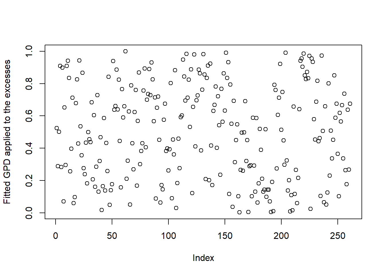
We can also consider a (more sophisticated) Q-Q plot for this task:
qq_plot(excess, FUN = function(p) qGPD(p, shape = xi.hat, scale = beta.hat),
        main = paste0("Q-Q plot for the fitted GPD(", round(xi.hat, 2),", ",
                      round(beta.hat, 2),") distribution")) # looks fine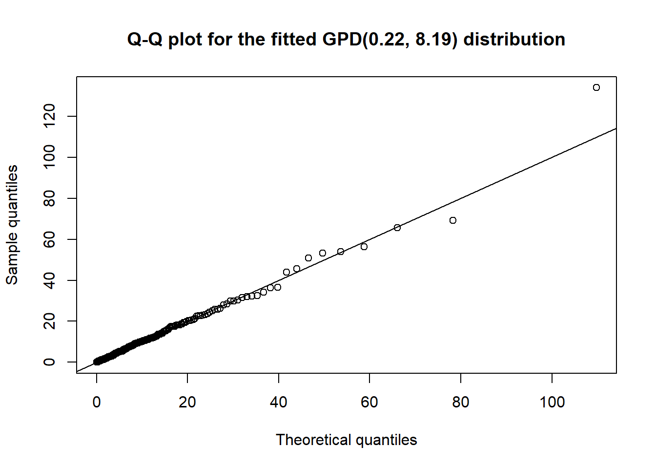
9.3 Graphical analysis
Compute historical losses (for creating a histogram); see risk.measure():
S. <- as.numeric(tail(S, n = 1)) # pick out last available stock prices ("today")
w. <- lambda * S. # weights tilde{w}
L <- loss_operator(X, weights = w.) # historical losses
summary(L) # get important statistics about the losses
## Min. 1st Qu. Median Mean 3rd Qu. Max.
## -135.7818406 -5.9714697 0.0000000 -0.1341209 5.8797401 147.9356414Plot a histogram of the losses including the VaR and ES estimates:
hist(L, breaks = "Scott", probability = TRUE, xlim = c(0, max(L, rm)), main = "",
     xlab = substitute("Losses L > 0 from"~sd~"to"~ed~"with"~
                                         widehat(VaR)[a] <= widehat(ES)[a],
                       list(sd = time[1], ed = time[2], a = alpha)), col = "gray90"); box() # histogram
lty <- c(3, 2, 1, 4, 5)
lwd <- c(1.6, 2, 1, 1.2, 1.2)
for(k in seq_len(nrow(rm)))
    abline(v = rm[k,], lty = lty[k], lwd = lwd[k]) # colored vertical lines indicating VaR and ES
legend("topright", bty = "n", inset = 0.02, lty = lty, lwd = lwd, legend = rownames(rm),
       title = as.expression(substitute(widehat(VaR)[a] <= widehat(ES)[a], list(a = alpha)))) # legend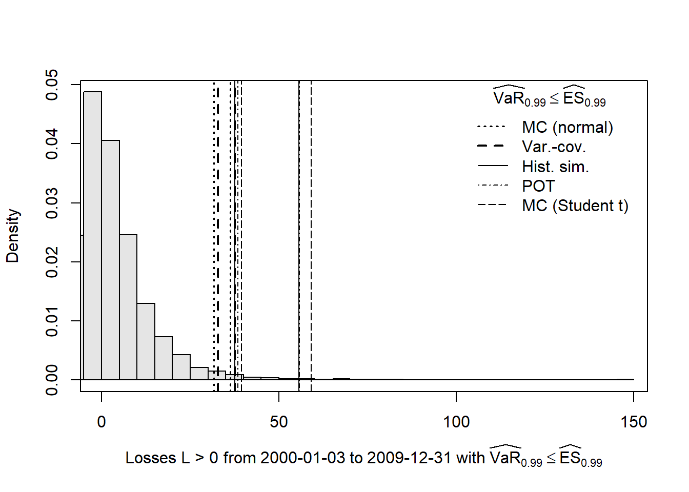
Results:
The Monte Carlo method based on a fitted multivariate normal distribution and the variance-covariance method lead to similar results (they both assume multivariate normal distributed risk-factor changes but differ in the computation of the loss distribution (analytical vs empirical)).
Both underestimate VaR and ES as estimated by historical simulation.
The historical simulation method implies that the loss distribution is more heavy-tailed. This is captured quite well by POT method and (possibly too well by) the Monte Carlo method for multivariate t distributed risk-factor changes (degrees of freedom are
MC.t$df\(\approx 2.4\)).It’s overall reassuring that several methods (historical simulation, POT method and – with slight departure for ES – MC for a Student \(t\)) lead to similar results. Somewhere in this range, one can then determine an adequate amount of risk capital.
9.4 Backtesting
Illustration of backtesting for a portfolio consisting of option on SP500 index
library(xts)
library(rugarch)
library(qrmtools)
library(qrmdata)

set.seed(271)

data(SP500)
data(VIX)

SP500.r = diff(log(SP500))['1990-01-03/']
VIX.r = diff(log(VIX))['1990-01-03/']
length(SP500.r)
## [1] 6552length(VIX.r)## [1] 6552X.d = merge(SP500.r, VIX.r)
X.w = apply.weekly(X.d, FUN = colSums)9.4.1 Backtesting Section
Recall key risk-factor changes for option price:
plot(as.matrix(X.d))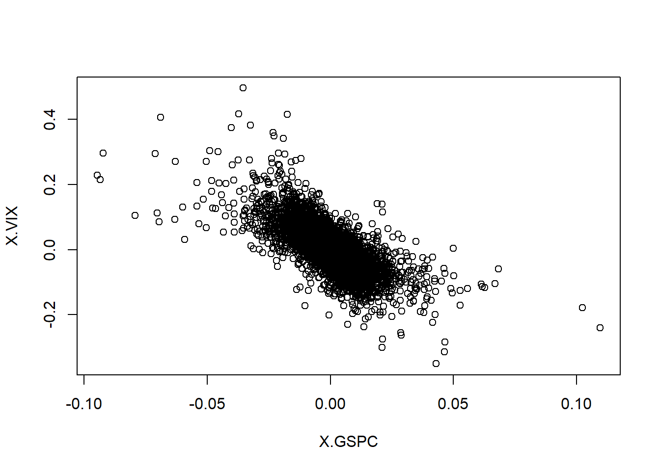
plot(as.matrix(X.w))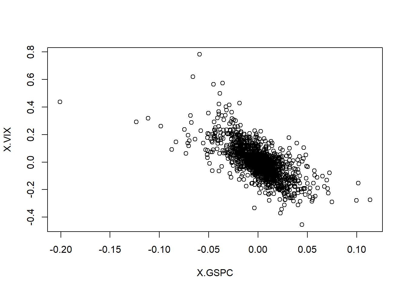
## Consider these as history of risk-factor changes up to present time.A bank is short a put option:
## Put option characteristics
K = 100
## Option currently "in the money": (K - S > 0) for put
S = 80
r = 0.03
sigma = 0.25
T = 1(Vt = -Black_Scholes(0, S, r, sigma, K, T, "put"))## [1] -19.81022858Vtplus1.d = -Black_Scholes(1/250, exp(log(S)+X.d[,1]), r, exp(log(sigma)+X.d[,2]), K, T, "put")
Vtplus1.w = -Black_Scholes(1/52, exp(log(S)+X.w[,1]), r, exp(log(sigma)+X.w[,2]), K, T, "put")
gains.d = Vtplus1.d-Vt
gains.w = Vtplus1.w-Vt
## The above time series are historically simulated "gains"
plot(gains.d)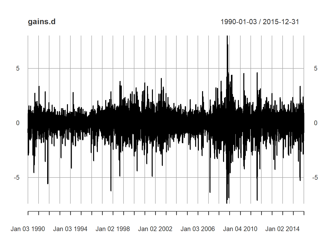
qqnorm(gains.d)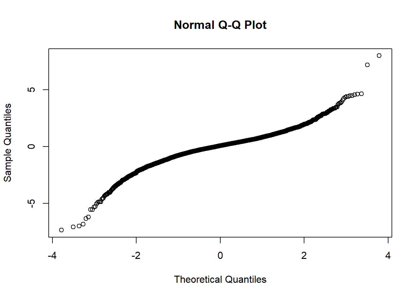
plot(gains.w)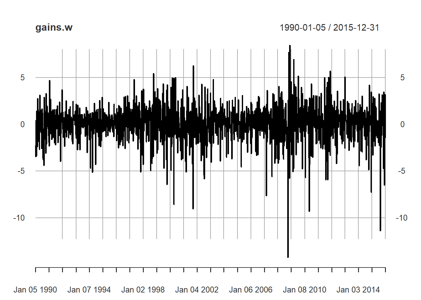
qqnorm(gains.w)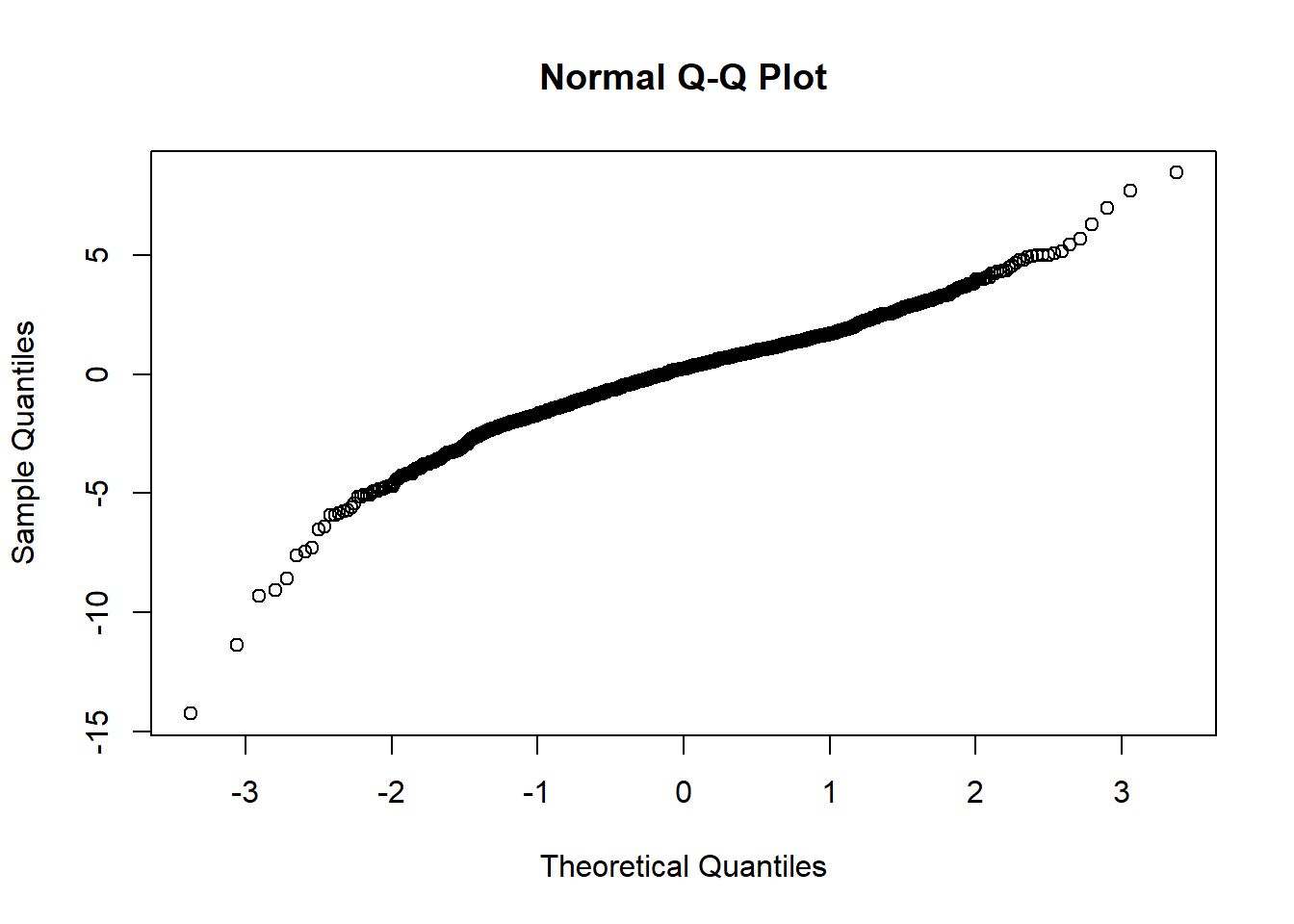
## These series bear all the signs of stochastic volatility
acf(gains.d)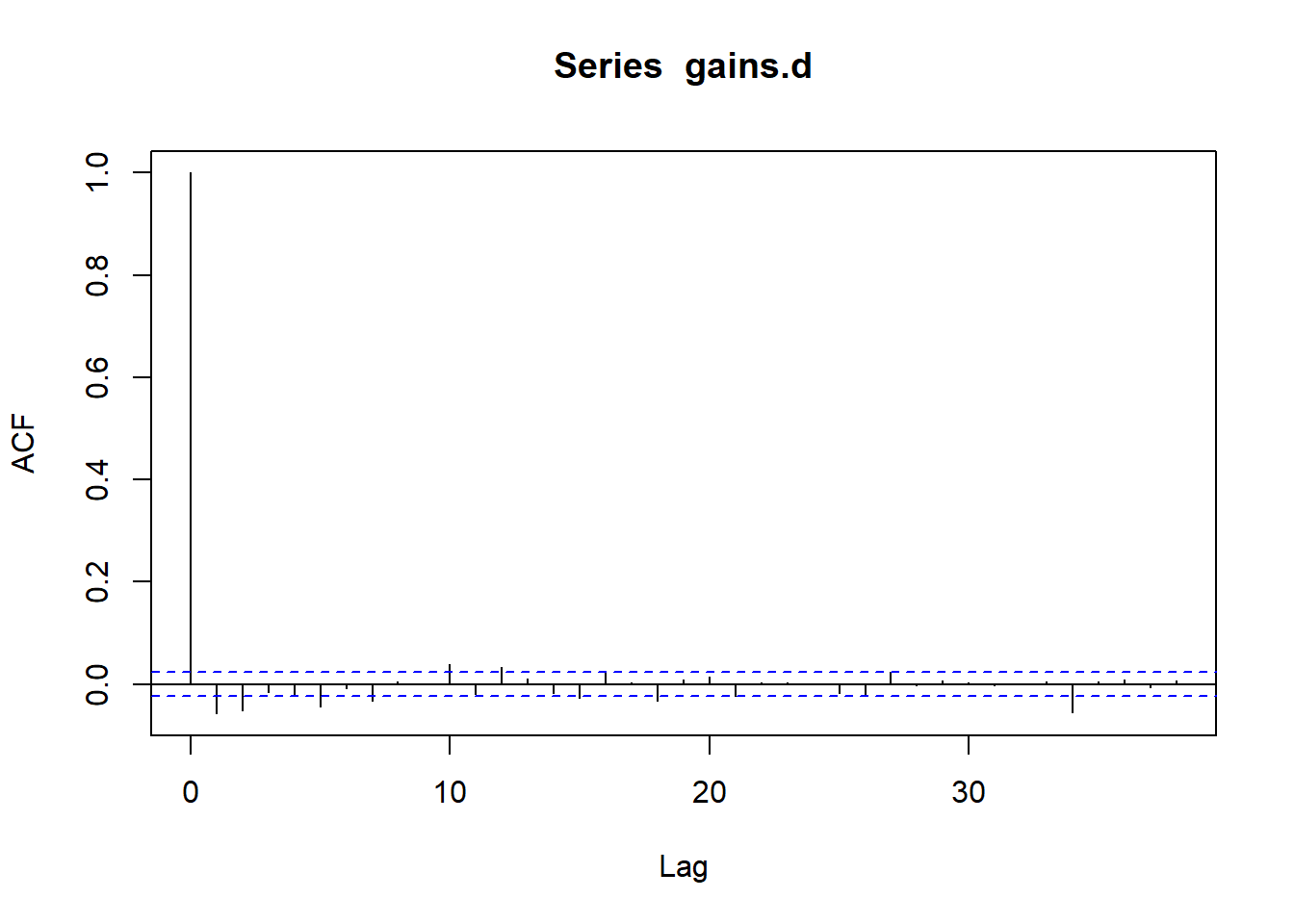
acf(abs(gains.d))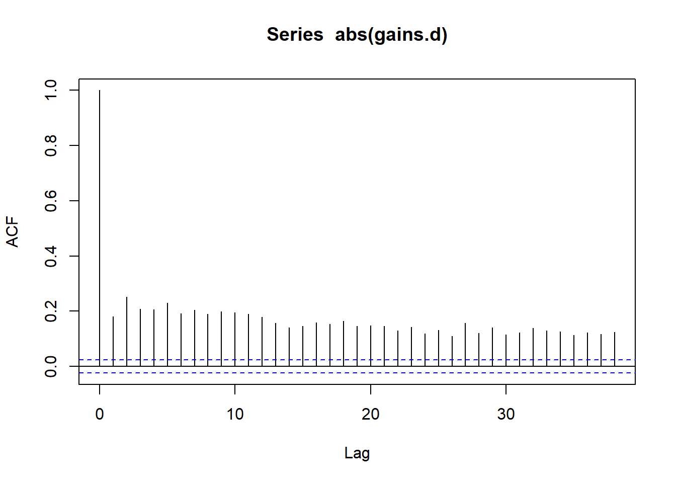
spec.n = ugarchspec(variance.model = list(model = "sGARCH", garchOrder = c(1,1)),
                     mean.model = list(armaOrder = c(1,1), include.mean = TRUE),
                     distribution.model = "norm")
spec.t = ugarchspec(variance.model = list(model = "sGARCH", garchOrder = c(1,1)),
                     mean.model = list(armaOrder = c(1,1), include.mean = TRUE), distribution.model = "std")
spec.tskew = ugarchspec(variance.model = list(model = "sGARCH", garchOrder = c(1,1)),
                         mean.model = list(armaOrder = c(1,1), include.mean = TRUE), distribution.model = "sstd")
## We now carry out a series of rolling out-of-sample VaR predictions
## We refit the model every 10 dayssystem.time(
roll.n <- ugarchroll(spec.n, gains.d, n.start = 1000, window.size = 1000, refit.every = 10,
refit.window = "moving", solver = "hybrid", calculate.VaR = TRUE,
VaR.alpha = c(0.05, 0.01))
) # ~= 1.5min## Warning in arima(data, order = c(modelinc[2], 0, modelinc[3]), include.mean =
## modelinc[1], : possible convergence problem: optim gave code = 1
## Warning in arima(data, order = c(modelinc[2], 0, modelinc[3]), include.mean =
## modelinc[1], : possible convergence problem: optim gave code = 1
## Warning in arima(data, order = c(modelinc[2], 0, modelinc[3]), include.mean =
## modelinc[1], : possible convergence problem: optim gave code = 1
## Warning in arima(data, order = c(modelinc[2], 0, modelinc[3]), include.mean =
## modelinc[1], : possible convergence problem: optim gave code = 1
## Warning in arima(data, order = c(modelinc[2], 0, modelinc[3]), include.mean =
## modelinc[1], : possible convergence problem: optim gave code = 1
## Warning in arima(data, order = c(modelinc[2], 0, modelinc[3]), include.mean =
## modelinc[1], : possible convergence problem: optim gave code = 1
## Warning in arima(data, order = c(modelinc[2], 0, modelinc[3]), include.mean =
## modelinc[1], : possible convergence problem: optim gave code = 1
## Warning in arima(data, order = c(modelinc[2], 0, modelinc[3]), include.mean =
## modelinc[1], : possible convergence problem: optim gave code = 1
## Warning in arima(data, order = c(modelinc[2], 0, modelinc[3]), include.mean =
## modelinc[1], : possible convergence problem: optim gave code = 1
## Warning in arima(data, order = c(modelinc[2], 0, modelinc[3]), include.mean =
## modelinc[1], : possible convergence problem: optim gave code = 1
## Warning in arima(data, order = c(modelinc[2], 0, modelinc[3]), include.mean =
## modelinc[1], : possible convergence problem: optim gave code = 1
## Warning in arima(data, order = c(modelinc[2], 0, modelinc[3]), include.mean =
## modelinc[1], : possible convergence problem: optim gave code = 1
## Warning in arima(data, order = c(modelinc[2], 0, modelinc[3]), include.mean =
## modelinc[1], : possible convergence problem: optim gave code = 1
## Warning in arima(data, order = c(modelinc[2], 0, modelinc[3]), include.mean =
## modelinc[1], : possible convergence problem: optim gave code = 1
## Warning in arima(data, order = c(modelinc[2], 0, modelinc[3]), include.mean =
## modelinc[1], : possible convergence problem: optim gave code = 1## user system elapsed
## 126.52 0.02 126.95show(roll.n)##
## *-------------------------------------*
## * GARCH Roll *
## *-------------------------------------*
## No.Refits : 556
## Refit Horizon : 10
## No.Forecasts : 5552
## GARCH Model : sGARCH(1,1)
## Distribution : norm
##
## Forecast Density:
## Mu Sigma Skew Shape Shape(GIG) Realized
## 1993-12-15 -0.0434 0.5675 0 0 0 -0.0961
## 1993-12-16 0.0308 0.5654 0 0 0 0.2723
## 1993-12-17 0.0031 0.5638 0 0 0 0.2813
## 1993-12-20 0.0202 0.5622 0 0 0 0.1254
## 1993-12-21 0.0027 0.5603 0 0 0 0.3256
## 1993-12-22 0.0224 0.5589 0 0 0 0.7490
##
## ..........................
## Mu Sigma Skew Shape Shape(GIG) Realized
## 2015-12-23 0.1627 1.0888 0 0 0 1.1434
## 2015-12-24 0.1040 1.0399 0 0 0 -0.1618
## 2015-12-28 0.1122 0.9298 0 0 0 -0.6115
## 2015-12-29 0.1428 0.8953 0 0 0 0.9527
## 2015-12-30 0.1079 0.8817 0 0 0 -0.9107
## 2015-12-31 0.1600 0.9134 0 0 0 -0.8966
##
## Elapsed: 2.115734883 minsplot(roll.n, which = 4)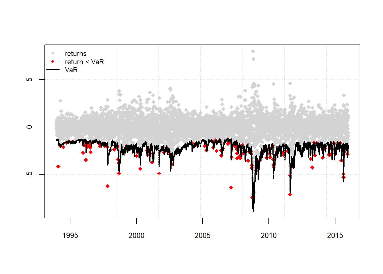
report(roll.n, type = "VaR", VaR.alpha = 0.01, conf.level = 0.95)## VaR Backtest Report
## ===========================================
## Model: sGARCH-norm
## Backtest Length: 5552
## Data:
##
## ==========================================
## alpha: 1%
## Expected Exceed: 55.5
## Actual VaR Exceed: 146
## Actual %: 2.6%
##
## Unconditional Coverage (Kupiec)
## Null-Hypothesis: Correct Exceedances
## LR.uc Statistic: 102.862
## LR.uc Critical: 3.841
## LR.uc p-value: 0
## Reject Null: YES
##
## Conditional Coverage (Christoffersen)
## Null-Hypothesis: Correct Exceedances and
## Independence of Failures
## LR.cc Statistic: 103.964
## LR.cc Critical: 5.991
## LR.cc p-value: 0
## Reject Null: YES## A little more detail on how VaR numbers are extracted
VaR.table.n = as.data.frame(roll.n, which = "VaR")
names(VaR.table.n)## [1] "alpha(5%)" "alpha(1%)" "realized"realized = VaR.table.n[,"realized"]
VaR05.n = VaR.table.n[,1]
VaR01.n = VaR.table.n[,2]
VaRTest(alpha = 0.01, actual = realized, VaR = VaR01.n)## $expected.exceed
## [1] 55
##
## $actual.exceed
## [1] 146
##
## $uc.H0
## [1] "Correct Exceedances"
##
## $uc.LRstat
## [1] 102.8617574
##
## $uc.critical
## [1] 3.841458821
##
## $uc.LRp
## [1] 0
##
## $uc.Decision
## [1] "Reject H0"
##
## $cc.H0
## [1] "Correct Exceedances & Independent"
##
## $cc.LRstat
## [1] 103.9640285
##
## $cc.critical
## [1] 5.991464547
##
## $cc.LRp
## [1] 0
##
## $cc.Decision
## [1] "Reject H0"par.n = as.data.frame(roll.n, which = "density")
names(par.n)## [1] "Mu" "Sigma" "Skew" "Shape" "Shape(GIG)"
## [6] "Realized"ES05.n = par.n$Mu - par.n$Sigma * ES_t(0.95, df = Inf)
ES01.n = par.n$Mu - par.n$Sigma * ES_t(0.99, df = Inf)
ESTest(alpha = 0.05, actual = realized, ES = ES05.n, VaR = VaR05.n)## $expected.exceed
## [1] 277
##
## $actual.exceed
## [1] 351
##
## $H1
## [1] "Mean of Excess Violations of VaR is greater than zero"
##
## $boot.p.value
## [1] NA
##
## $p.value
## [1] 4.329869796e-15
##
## $Decision
## [1] "Reject H0"ESTest(alpha = 0.01, actual = realized, ES = ES01.n, VaR = VaR01.n)## $expected.exceed
## [1] 55
##
## $actual.exceed
## [1] 146
##
## $H1
## [1] "Mean of Excess Violations of VaR is greater than zero"
##
## $boot.p.value
## [1] NA
##
## $p.value
## [1] 5.096204903e-09
##
## $Decision
## [1] "Reject H0"## Now try fitting the Student t Model
system.time(
roll.t <- ugarchroll(spec.t, gains.d, n.start = 1000, window.size = 1000, refit.every = 10,
refit.window = "moving", solver = "hybrid", calculate.VaR = TRUE,
VaR.alpha = c(0.05, 0.01))
) # ~= 2.5min## Warning in arima(data, order = c(modelinc[2], 0, modelinc[3]), include.mean =
## modelinc[1], : possible convergence problem: optim gave code = 1
## Warning in arima(data, order = c(modelinc[2], 0, modelinc[3]), include.mean =
## modelinc[1], : possible convergence problem: optim gave code = 1
## Warning in arima(data, order = c(modelinc[2], 0, modelinc[3]), include.mean =
## modelinc[1], : possible convergence problem: optim gave code = 1
## Warning in arima(data, order = c(modelinc[2], 0, modelinc[3]), include.mean =
## modelinc[1], : possible convergence problem: optim gave code = 1
## Warning in arima(data, order = c(modelinc[2], 0, modelinc[3]), include.mean =
## modelinc[1], : possible convergence problem: optim gave code = 1
## Warning in arima(data, order = c(modelinc[2], 0, modelinc[3]), include.mean =
## modelinc[1], : possible convergence problem: optim gave code = 1
## Warning in arima(data, order = c(modelinc[2], 0, modelinc[3]), include.mean =
## modelinc[1], : possible convergence problem: optim gave code = 1
## Warning in arima(data, order = c(modelinc[2], 0, modelinc[3]), include.mean =
## modelinc[1], : possible convergence problem: optim gave code = 1
## Warning in arima(data, order = c(modelinc[2], 0, modelinc[3]), include.mean =
## modelinc[1], : possible convergence problem: optim gave code = 1
## Warning in arima(data, order = c(modelinc[2], 0, modelinc[3]), include.mean =
## modelinc[1], : possible convergence problem: optim gave code = 1
## Warning in arima(data, order = c(modelinc[2], 0, modelinc[3]), include.mean =
## modelinc[1], : possible convergence problem: optim gave code = 1
## Warning in arima(data, order = c(modelinc[2], 0, modelinc[3]), include.mean =
## modelinc[1], : possible convergence problem: optim gave code = 1
## Warning in arima(data, order = c(modelinc[2], 0, modelinc[3]), include.mean =
## modelinc[1], : possible convergence problem: optim gave code = 1
## Warning in arima(data, order = c(modelinc[2], 0, modelinc[3]), include.mean =
## modelinc[1], : possible convergence problem: optim gave code = 1
## Warning in arima(data, order = c(modelinc[2], 0, modelinc[3]), include.mean =
## modelinc[1], : possible convergence problem: optim gave code = 1## user system elapsed
## 198.64 0.01 198.95show(roll.t)##
## *-------------------------------------*
## * GARCH Roll *
## *-------------------------------------*
## No.Refits : 556
## Refit Horizon : 10
## No.Forecasts : 5552
## GARCH Model : sGARCH(1,1)
## Distribution : std
##
## Forecast Density:
## Mu Sigma Skew Shape Shape(GIG) Realized
## 1993-12-15 0.0257 0.5673 0 4.43 0 -0.0961
## 1993-12-16 0.0673 0.5634 0 4.43 0 0.2723
## 1993-12-17 0.0478 0.5599 0 4.43 0 0.2813
## 1993-12-20 0.0611 0.5567 0 4.43 0 0.1254
## 1993-12-21 0.0486 0.5527 0 4.43 0 0.3256
## 1993-12-22 0.0615 0.5499 0 4.43 0 0.7490
##
## ..........................
## Mu Sigma Skew Shape Shape(GIG) Realized
## 2015-12-23 0.1987 1.1239 0 4.8900 0 1.1434
## 2015-12-24 0.1236 1.0645 0 4.8900 0 -0.1618
## 2015-12-28 0.1351 0.9394 0 4.8900 0 -0.6115
## 2015-12-29 0.1752 0.9081 0 4.8900 0 0.9527
## 2015-12-30 0.1272 0.8927 0 4.8923 0 -0.9107
## 2015-12-31 0.1919 0.9403 0 4.8923 0 -0.8966
##
## Elapsed: 3.315772251 minsplot(roll.t, which = 4)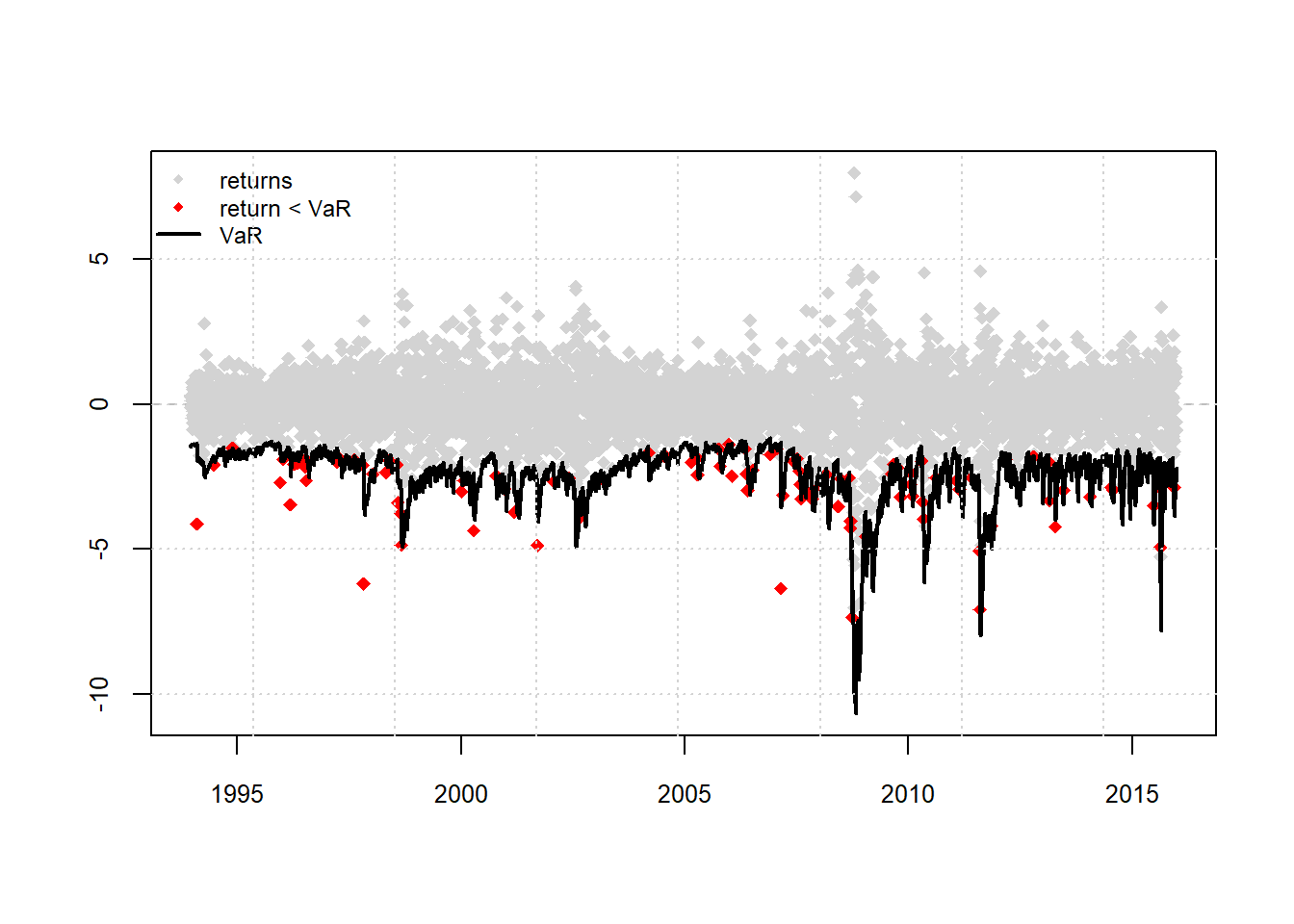
report(roll.t, type = "VaR", VaR.alpha = 0.01, conf.level = 0.95)## VaR Backtest Report
## ===========================================
## Model: sGARCH-std
## Backtest Length: 5552
## Data:
##
## ==========================================
## alpha: 1%
## Expected Exceed: 55.5
## Actual VaR Exceed: 105
## Actual %: 1.9%
##
## Unconditional Coverage (Kupiec)
## Null-Hypothesis: Correct Exceedances
## LR.uc Statistic: 35.302
## LR.uc Critical: 3.841
## LR.uc p-value: 0
## Reject Null: YES
##
## Conditional Coverage (Christoffersen)
## Null-Hypothesis: Correct Exceedances and
## Independence of Failures
## LR.cc Statistic: 35.769
## LR.cc Critical: 5.991
## LR.cc p-value: 0
## Reject Null: YESVaR.table.t = as.data.frame(roll.t, which = "VaR")
names(VaR.table.t)## [1] "alpha(5%)" "alpha(1%)" "realized"realized = VaR.table.t[,"realized"]
VaR05.t = VaR.table.t[,1]
VaR01.t = VaR.table.t[,2]par.t = as.data.frame(roll.t, which = "density")
names(par.t)## [1] "Mu" "Sigma" "Skew" "Shape" "Shape(GIG)"
## [6] "Realized"ES05.t = par.t$Mu - par.t$Sigma * ES_t(0.95, df = par.t$Shape, scale = TRUE)
ES01.t = par.t$Mu - par.t$Sigma * ES_t(0.99, df = par.t$Shape, scale = TRUE)
ESTest(alpha = 0.05, actual = realized, ES = ES05.t, VaR = VaR05.t)## $expected.exceed
## [1] 277
##
## $actual.exceed
## [1] 406
##
## $H1
## [1] "Mean of Excess Violations of VaR is greater than zero"
##
## $boot.p.value
## [1] NA
##
## $p.value
## [1] 1
##
## $Decision
## [1] "Fail to Reject H0"ESTest(alpha = 0.01, actual = realized, ES = ES01.t, VaR = VaR01.t)## $expected.exceed
## [1] 55
##
## $actual.exceed
## [1] 105
##
## $H1
## [1] "Mean of Excess Violations of VaR is greater than zero"
##
## $boot.p.value
## [1] NA
##
## $p.value
## [1] 1
##
## $Decision
## [1] "Fail to Reject H0"## Now try skew-t innovations. Caution: slow
system.time(
roll.tskew <- ugarchroll(spec.tskew, gains.d, n.start = 1000, window.size = 1000, refit.every = 10,
refit.window = "moving", solver = "hybrid", calculate.VaR = TRUE,
VaR.alpha = c(0.05, 0.01))
) # ~= 4min## Warning in arima(data, order = c(modelinc[2], 0, modelinc[3]), include.mean =
## modelinc[1], : possible convergence problem: optim gave code = 1
## Warning in arima(data, order = c(modelinc[2], 0, modelinc[3]), include.mean =
## modelinc[1], : possible convergence problem: optim gave code = 1
## Warning in arima(data, order = c(modelinc[2], 0, modelinc[3]), include.mean =
## modelinc[1], : possible convergence problem: optim gave code = 1
## Warning in arima(data, order = c(modelinc[2], 0, modelinc[3]), include.mean =
## modelinc[1], : possible convergence problem: optim gave code = 1
## Warning in arima(data, order = c(modelinc[2], 0, modelinc[3]), include.mean =
## modelinc[1], : possible convergence problem: optim gave code = 1
## Warning in arima(data, order = c(modelinc[2], 0, modelinc[3]), include.mean =
## modelinc[1], : possible convergence problem: optim gave code = 1
## Warning in arima(data, order = c(modelinc[2], 0, modelinc[3]), include.mean =
## modelinc[1], : possible convergence problem: optim gave code = 1
## Warning in arima(data, order = c(modelinc[2], 0, modelinc[3]), include.mean =
## modelinc[1], : possible convergence problem: optim gave code = 1
## Warning in arima(data, order = c(modelinc[2], 0, modelinc[3]), include.mean =
## modelinc[1], : possible convergence problem: optim gave code = 1
## Warning in arima(data, order = c(modelinc[2], 0, modelinc[3]), include.mean =
## modelinc[1], : possible convergence problem: optim gave code = 1
## Warning in arima(data, order = c(modelinc[2], 0, modelinc[3]), include.mean =
## modelinc[1], : possible convergence problem: optim gave code = 1
## Warning in arima(data, order = c(modelinc[2], 0, modelinc[3]), include.mean =
## modelinc[1], : possible convergence problem: optim gave code = 1
## Warning in arima(data, order = c(modelinc[2], 0, modelinc[3]), include.mean =
## modelinc[1], : possible convergence problem: optim gave code = 1
## Warning in arima(data, order = c(modelinc[2], 0, modelinc[3]), include.mean =
## modelinc[1], : possible convergence problem: optim gave code = 1
## Warning in arima(data, order = c(modelinc[2], 0, modelinc[3]), include.mean =
## modelinc[1], : possible convergence problem: optim gave code = 1## user system elapsed
## 333.88 0.06 334.28show(roll.tskew)##
## *-------------------------------------*
## * GARCH Roll *
## *-------------------------------------*
## No.Refits : 556
## Refit Horizon : 10
## No.Forecasts : 5552
## GARCH Model : sGARCH(1,1)
## Distribution : sstd
##
## Forecast Density:
## Mu Sigma Skew Shape Shape(GIG) Realized
## 1993-12-15 -0.0006 0.5614 0.8506 4.7558 0 -0.0961
## 1993-12-16 0.0323 0.5573 0.8506 4.7558 0 0.2723
## 1993-12-17 0.0163 0.5539 0.8506 4.7558 0 0.2813
## 1993-12-20 0.0274 0.5508 0.8506 4.7558 0 0.1254
## 1993-12-21 0.0171 0.5468 0.8506 4.7558 0 0.3256
## 1993-12-22 0.0276 0.5442 0.8506 4.7558 0 0.7490
##
## ..........................
## Mu Sigma Skew Shape Shape(GIG) Realized
## 2015-12-23 0.1662 1.0671 0.7457 5.9171 0 1.1434
## 2015-12-24 0.0639 1.0218 0.7457 5.9171 0 -0.1618
## 2015-12-28 0.0799 0.9096 0.7457 5.9171 0 -0.6115
## 2015-12-29 0.1347 0.8737 0.7457 5.9171 0 0.9527
## 2015-12-30 0.0699 0.8650 0.7417 6.0082 0 -0.9107
## 2015-12-31 0.1536 0.8932 0.7417 6.0082 0 -0.8966
##
## Elapsed: 5.571302915 minsplot(roll.tskew, which = 4)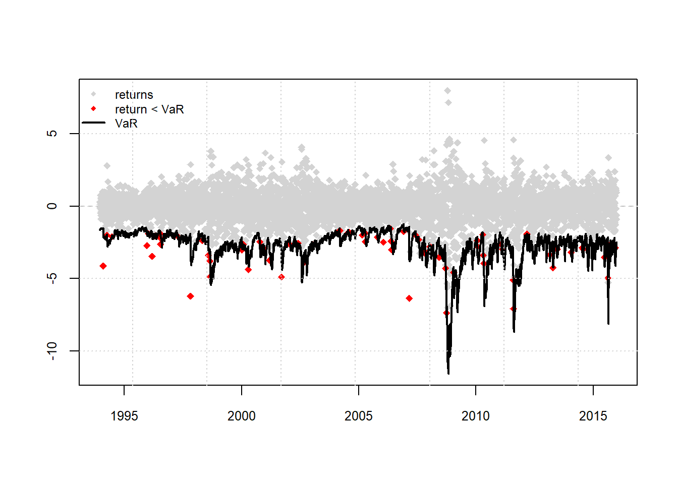
report(roll.tskew, type = "VaR", VaR.alpha = 0.01, conf.level = 0.95)## VaR Backtest Report
## ===========================================
## Model: sGARCH-sstd
## Backtest Length: 5552
## Data:
##
## ==========================================
## alpha: 1%
## Expected Exceed: 55.5
## Actual VaR Exceed: 72
## Actual %: 1.3%
##
## Unconditional Coverage (Kupiec)
## Null-Hypothesis: Correct Exceedances
## LR.uc Statistic: 4.518
## LR.uc Critical: 3.841
## LR.uc p-value: 0.034
## Reject Null: YES
##
## Conditional Coverage (Christoffersen)
## Null-Hypothesis: Correct Exceedances and
## Independence of Failures
## LR.cc Statistic: 5.465
## LR.cc Critical: 5.991
## LR.cc p-value: 0.065
## Reject Null: NO