Chapter 3 Empirical Properties of Financial Data
3.1 Exploring financial time series
Loading, exploring, merging, aggregating and presenting financial time series.
library(xts)
library(qrmdata)
library(qrmtools)
we denote a return series by \(X_1,..., X_n\) and assume that the returns have been formed by logarithmic differencing of a price, index or exchange-rate series \((S_t)_{t=0,1,...,n}\), so \(X_t = \ln(S_t/S_{t−1}), \ t = 1,...,n\).
3.1.1 Stock prices
Dow Jones stock price data:
data("DJ_const")
str(DJ_const)
## An 'xts' object on 1962-01-02/2015-12-31 containing:
## Data: num [1:13595, 1:30] NA NA NA NA NA NA NA NA NA NA ...
## - attr(*, "dimnames")=List of 2
## ..$ : NULL
## ..$ : chr [1:30] "AAPL" "AXP" "BA" "CAT" ...
## Indexed by objects of class: [Date] TZ: UTC
## xts Attributes:
## List of 2
## $ src : chr "yahoo"
## $ updated: POSIXct[1:1], format: "2016-01-03 03:51:40"We extract a time period and take the first 10 stocks:
DJdata = DJ_const['2006-12-29/2015-12-31', 1:10]Use plot for zoo objects to get multiple plots:
plot.zoo(DJdata, xlab = "Time", main = "DJ (10 component series)")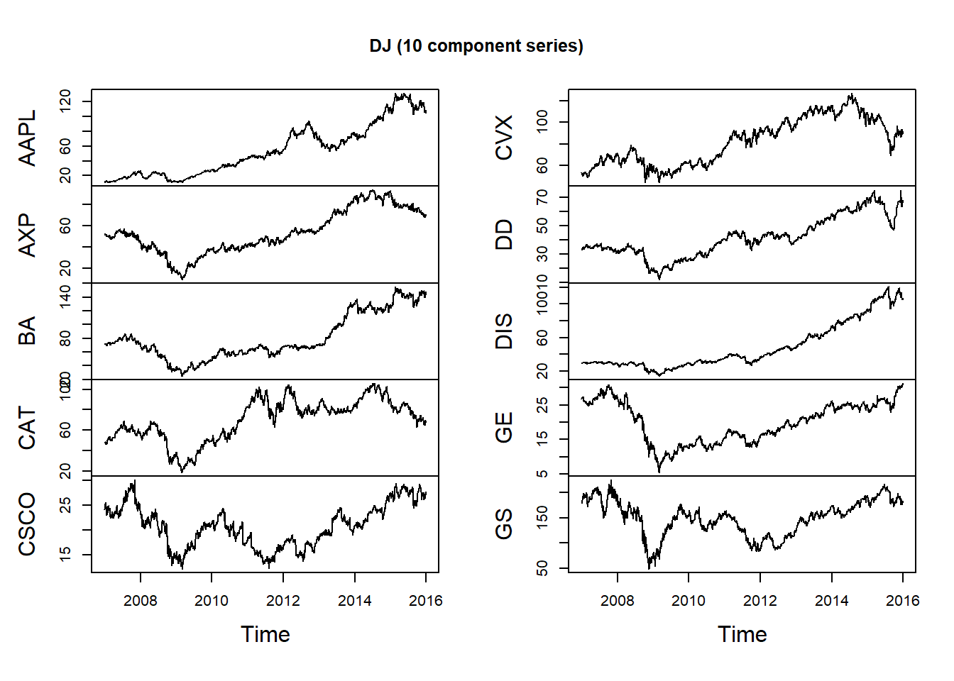
X = returns(DJdata) # or diff(log(DJdata))[-1,]
head(X)
## AAPL AXP BA CAT
## 2007-01-03 -0.012334120897 -0.0026472451560 0.003707673683 -0.002775765300
## 2007-01-04 0.021952926933 -0.0073163443921 0.004029116838 -0.002619510253
## 2007-01-05 -0.007146655399 -0.0132718850725 -0.004253386164 -0.012869324130
## 2007-01-08 0.004926129847 0.0094260573927 -0.002358358218 0.001161734403
## 2007-01-09 0.079799667183 -0.0063865234723 -0.010625198954 0.005458576326
## 2007-01-10 0.046745828277 -0.0006746670108 0.014328641844 -0.004961130145
## CSCO CVX DD DIS
## 2007-01-03 0.0145298305107 -0.035436194360 0.0067520100735 -0.002044583519
## 2007-01-04 0.0259847195971 -0.009770024128 -0.0069572791680 0.007863637421
## 2007-01-05 0.0003513138828 0.003834480727 -0.0134369575441 -0.008156047838
## 2007-01-08 0.0056042225031 0.012676130506 0.0004161386786 0.009026136834
## 2007-01-09 -0.0056042225031 -0.011542923051 0.0064282683029 -0.001450278326
## 2007-01-10 0.0073491451876 -0.017423932059 -0.0024834283353 0.001160410990
## GE GS
## 2007-01-03 0.0202188821092 0.006848800109
## 2007-01-04 -0.0058109041379 -0.009360107362
## 2007-01-05 -0.0050457874538 0.001005264216
## 2007-01-08 -0.0002663387811 0.023239502819
## 2007-01-09 0.0000000000000 0.001716517333
## 2007-01-10 0.0002663387811 0.019554703696plot.zoo(X, xlab = "Time", main = "Log-returns of 10 DJ component series")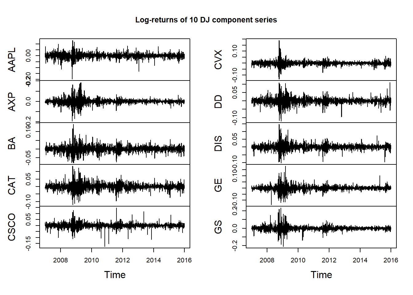
Volatility clustering is the tendency for extreme returns to be followed by other extreme returns, although not necessarily with the same sign.
Aggregating log returns by summation for each column:
## Weekly
X.w = apply.weekly(X, FUN = colSums)
dim(X.w)
## [1] 470 10plot.zoo(X.w, type = "h", xlab = "Time", main = "Weekly log-returns") # 'h' = histogram = vertical lines only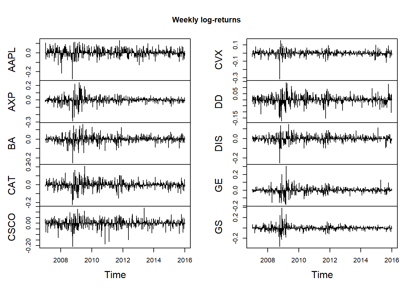
## Monthly
X.m = apply.monthly(X, FUN = colSums)
dim(X.m)
## [1] 108 10plot.zoo(X.m, type = "h", xlab = "Time", main = "Monthly log-returns")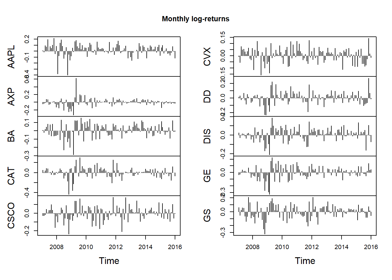
## Quarterly
X.q = apply.quarterly(X, FUN = colSums)
dim(X.q)
## [1] 36 10plot.zoo(X.q, type = "h", xlab = "Time", main = "Quarterly log-returns")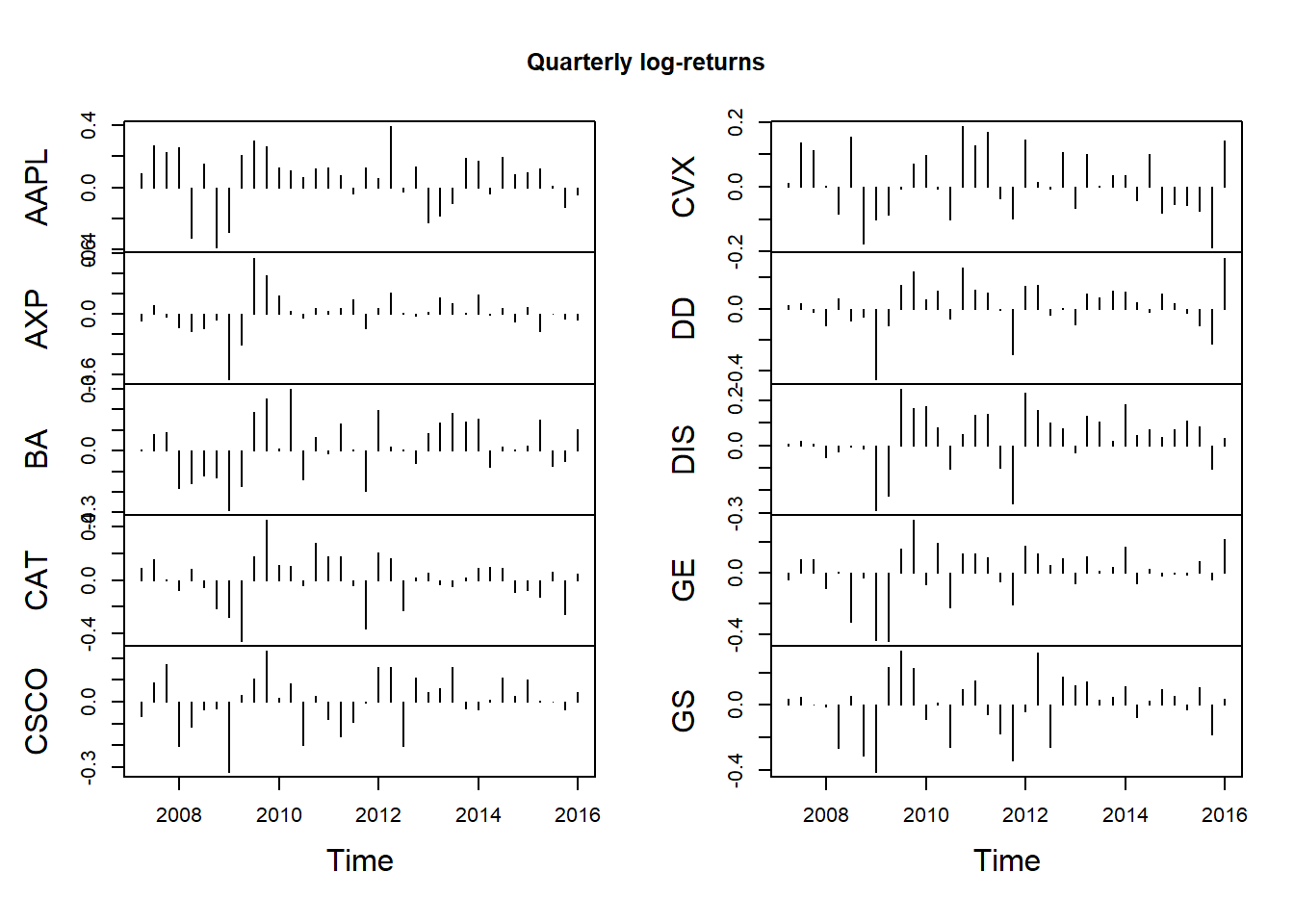
3.1.2 Stock indexes
Load stock index data:
data("SP500") # S&P 500
data("FTSE") # FTSE
data("SMI") # SMI
plot.zoo(SP500, xlab = "Time", ylab = "S&P 500")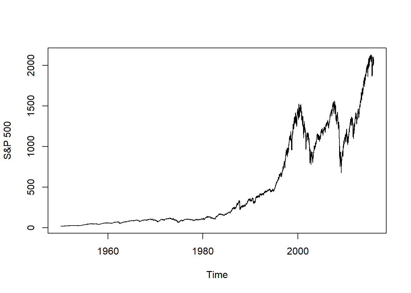
Merge the three time series:
all = merge(SP500, FTSE, SMI)
nms = c("S&P 500", "FTSE", "SMI")
colnames(all) = nms
plot.zoo(all, xlab = "Time", main = "All")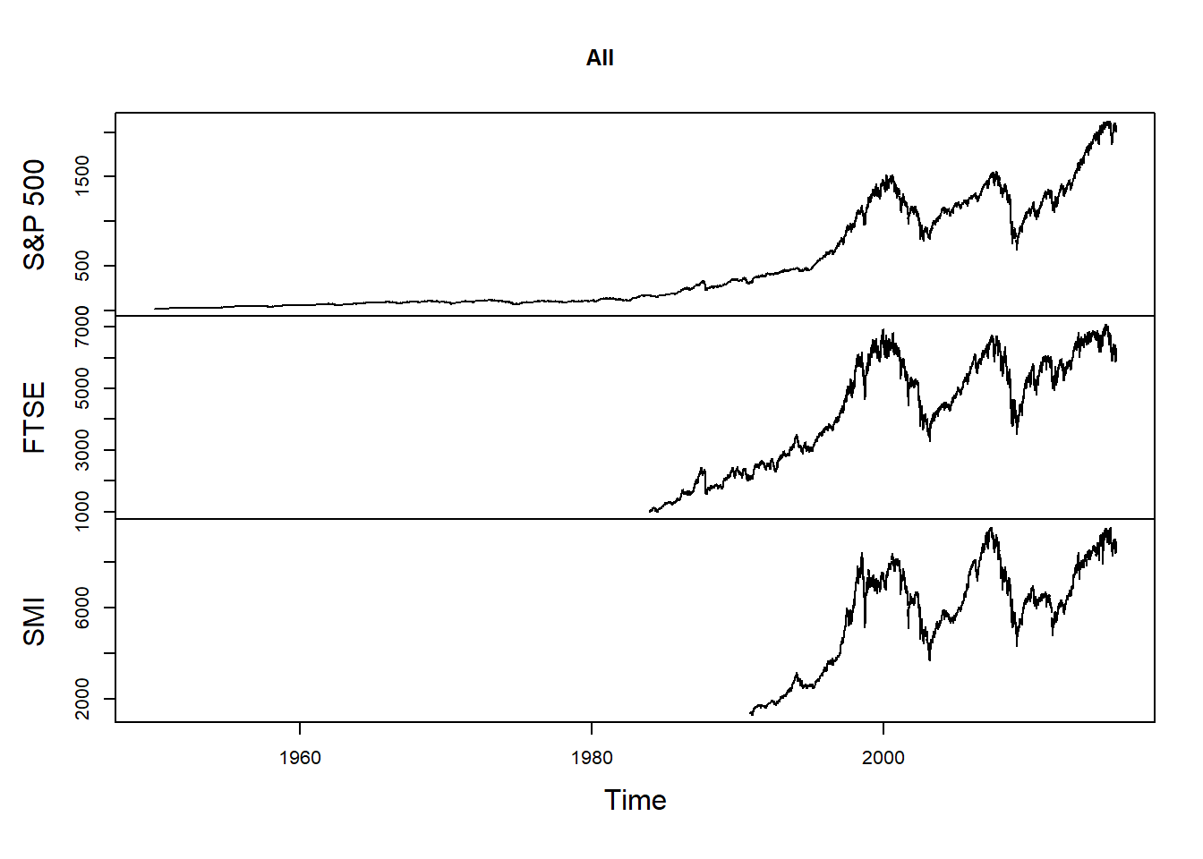
Merge and retain only days where all three time series are available:
all.avail = merge(SP500, FTSE, SMI, all = FALSE)
colnames(all.avail) = nms
plot.zoo(all.avail, xlab = "Time", main = "All available")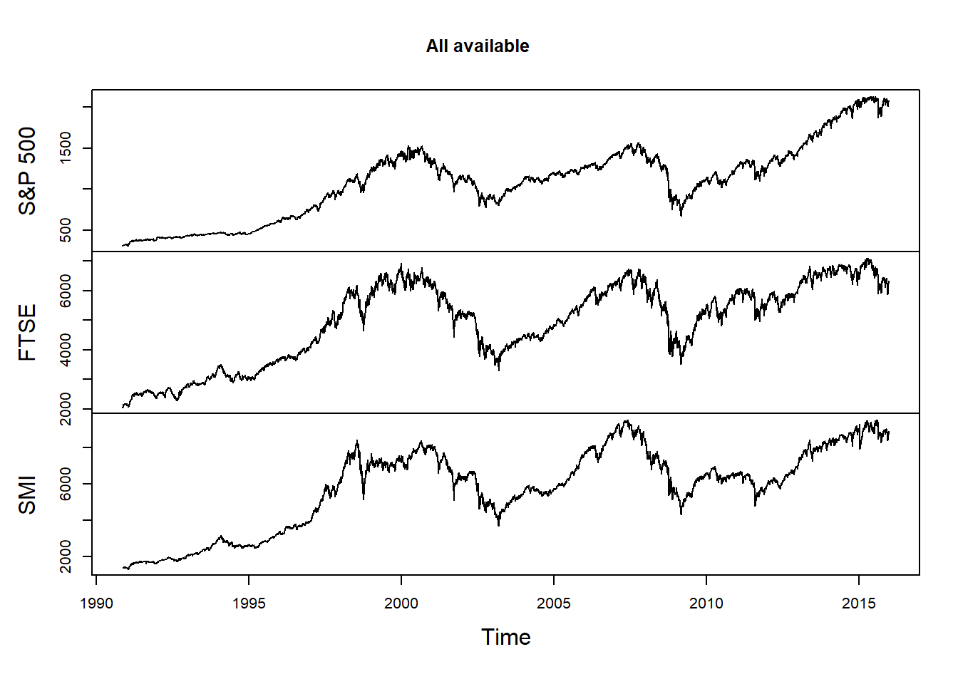
Compute returns:
SP500.X = returns(SP500)
FTSE.X  = returns(FTSE)
SMI.X   = returns(SMI)
X = merge(SP500.X, FTSE.X, SMI.X, all = FALSE)
colnames(X) = nms
plot.zoo(X, xlab = "Time", main = "Log-returns")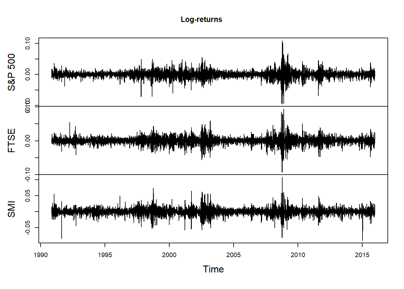
pairs(as.zoo(X), gap = 0, cex = 0.4)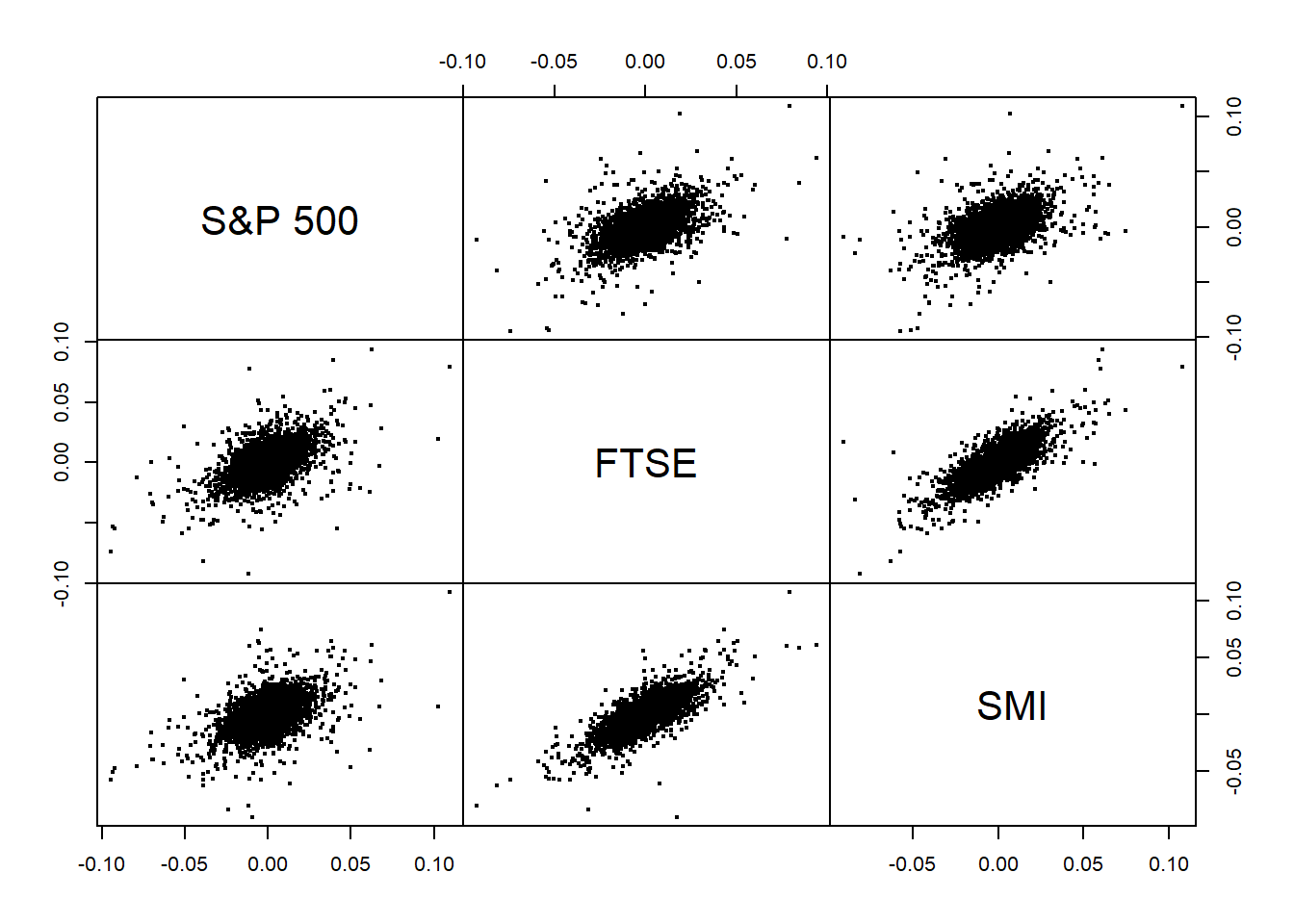
Aggregating:
## By week
X.w = apply.weekly(X, FUN = colSums)
plot.zoo(X.w, xlab = "Time", main = "Weekly log-returns", type = "h")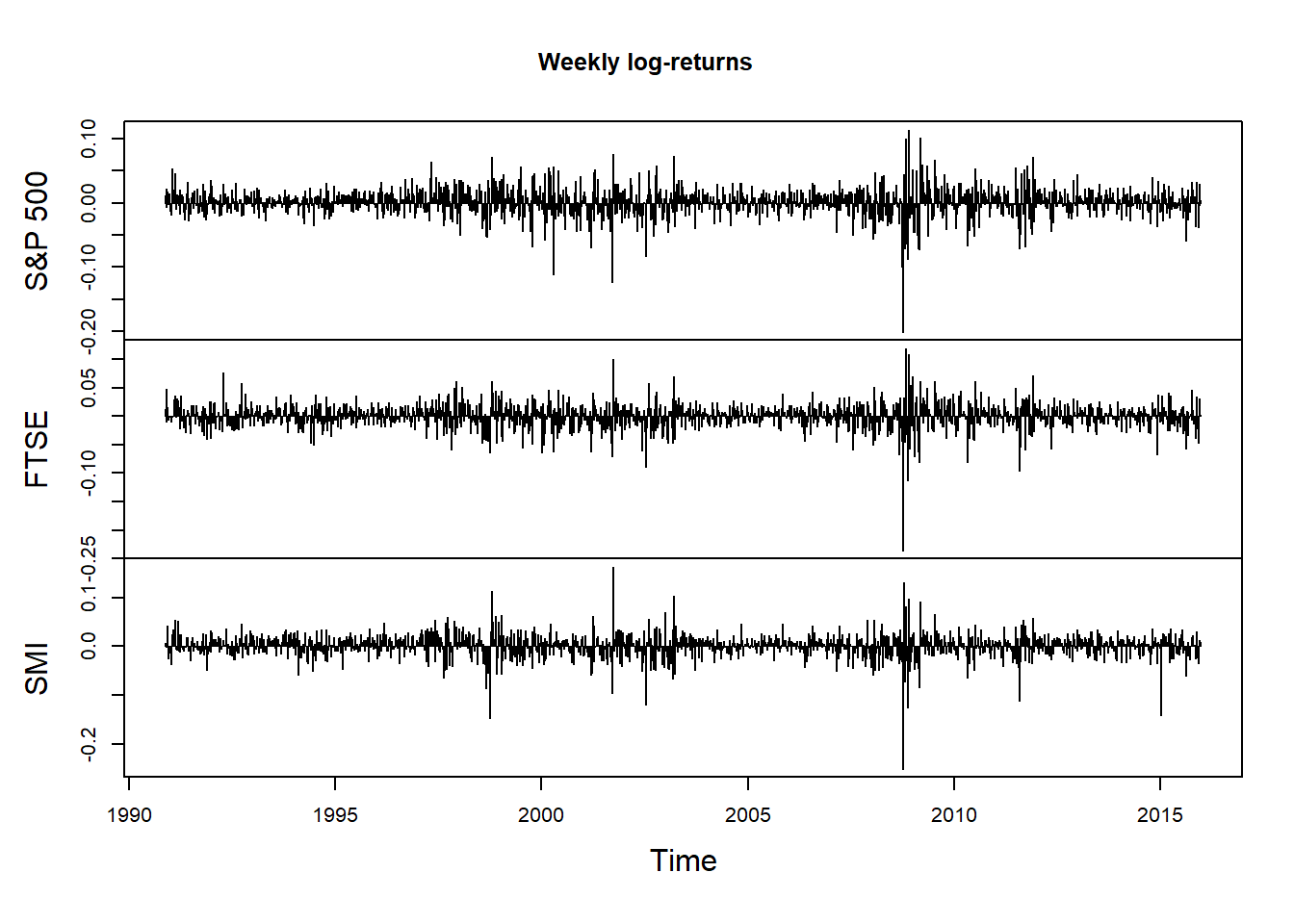
## By month
X.m = apply.monthly(X, FUN = colSums)
plot.zoo(X.m, xlab = "Time", main = "Monthly log-returns", type = "h")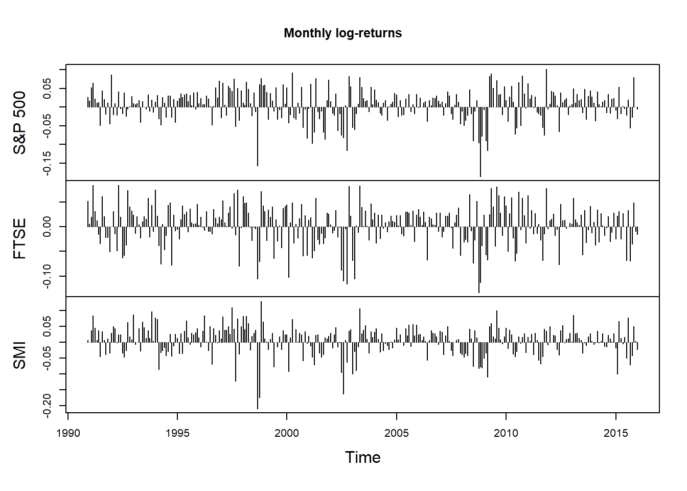
3.1.3 Exchange rates
Load exchange rate data:
data("GBP_USD") # 1 GBP in USD
data("EUR_USD") # 1 EUR in USD
data("JPY_USD") # 1 JPY in USD
data("CHF_USD") # 1 CHF in USD
FX = merge(GBP_USD, EUR_USD, JPY_USD, CHF_USD)
head(FX)
## GBP.USD EUR.USD JPY.USD CHF.USD
## 2000-01-01 1.6170 1.0057 0.009785693316 0.6285
## 2000-01-02 1.6170 1.0055 0.009789525208 0.6272
## 2000-01-03 1.6370 1.0258 0.009838646202 0.6392
## 2000-01-04 1.6357 1.0309 0.009682416731 0.6427
## 2000-01-05 1.6418 1.0322 0.009588647042 0.6432
## 2000-01-06 1.6466 1.0318 0.009502090460 0.6431plot.zoo(FX, xlab = "Time", main = "Exchange rates to USD")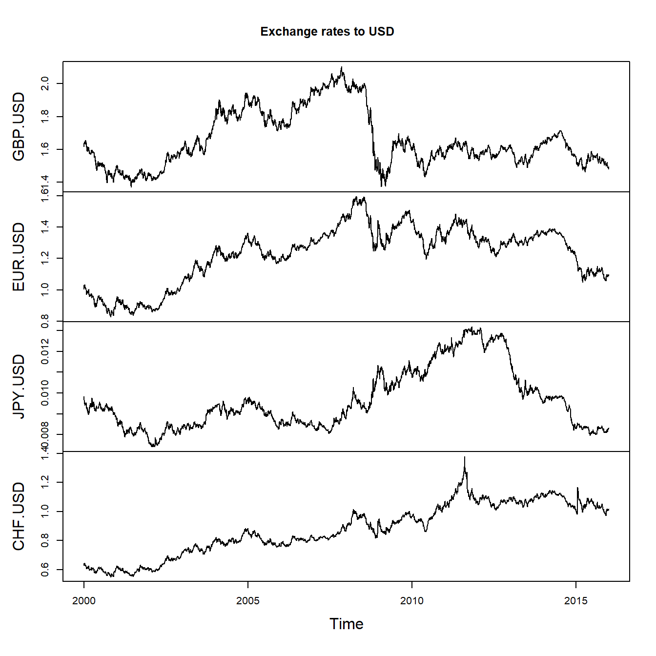
X = returns(FX)
plot.zoo(X, xlab = "Time", main = "Log-returns of exchange rates to USD",
         col = c("black", "royalblue3", "maroon3", "darkorange2"))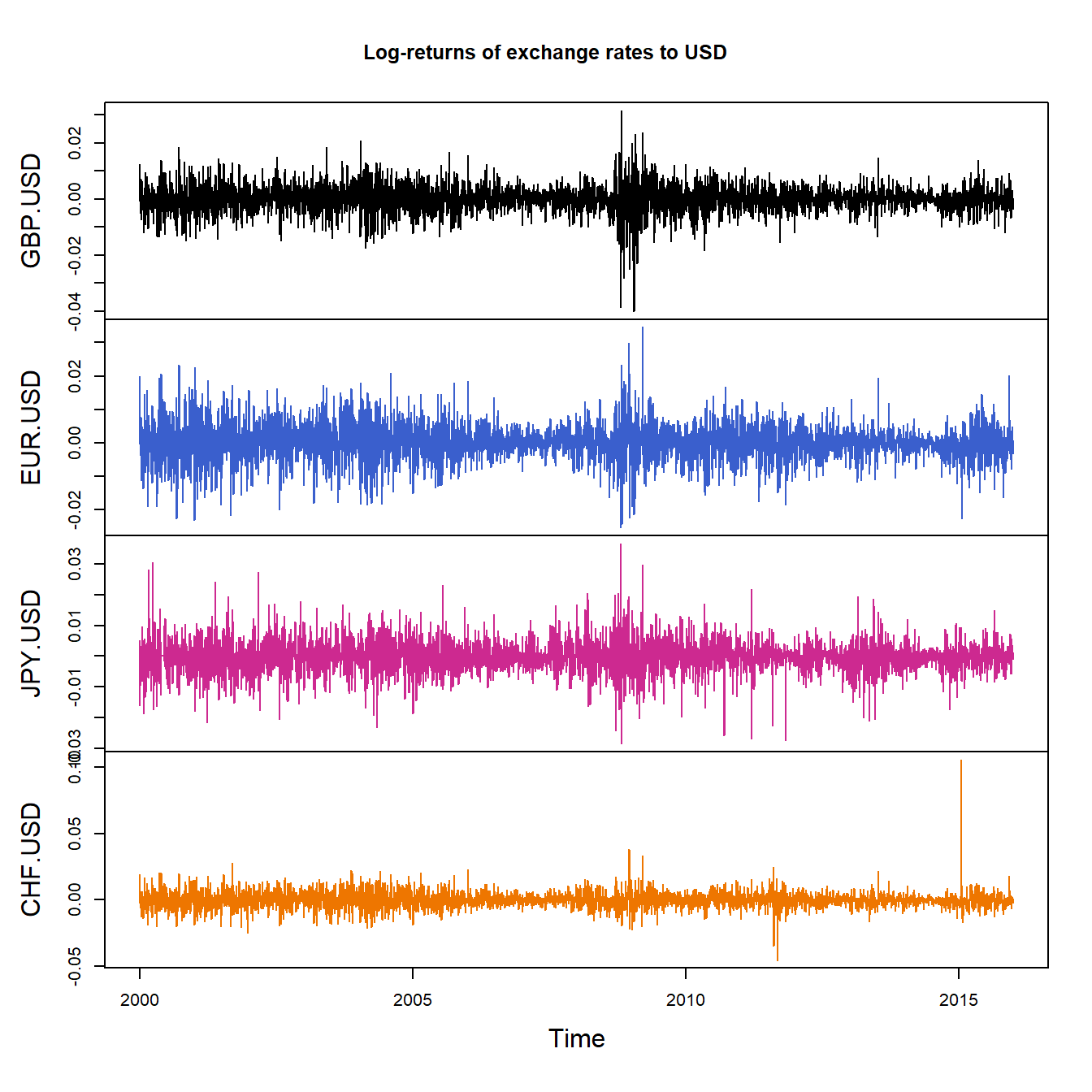
3.1.4 Zero-coupon bond yields
Load zero-coupon bond yield data (in USD):
Note: Typically, \[ \text{yield} = \left(\left(\frac{\text{face value}}{\text{current bond price}}\right)^{\frac{1}{\text{maturity}}} - 1\right) \cdot 100\% \] (as \(\text{face value} = \text{current price} \cdot (1 + \text{yield})^\text{maturity}\)
data("ZCB_USD")
dim(ZCB_USD) # => 30-dimensional; each dimension is a maturity
## [1] 7509 30head(ZCB_USD)## 1y 2y 3y 4y 5y 6y 7y 8y 9y
## 1985-11-25 7.8551 8.3626 8.7469 9.0408 9.2686 9.4481 9.5924 9.7110 9.8108
## 1985-11-26 7.8527 8.3575 8.7420 9.0376 9.2677 9.4494 9.5956 9.7154 9.8158
## 1985-11-27 7.8425 8.3522 8.7339 9.0231 9.2453 9.4193 9.5586 9.6727 9.7688
## 1985-11-29 7.7914 8.3148 8.6991 8.9852 9.2024 9.3712 9.5061 9.6172 9.7115
## 1985-12-02 7.8176 8.3457 8.7359 9.0294 9.2550 9.4327 9.5766 9.6962 9.7983
## 1985-12-03 7.8527 8.3679 8.7540 9.0476 9.2746 9.4535 9.5974 9.7156 9.8148
## 10y 11y 12y 13y 14y 15y 16y 17y
## 1985-11-25 9.8969 9.9727 10.0408 10.1029 10.1605 10.2143 10.2649 10.3128
## 1985-11-26 9.9015 9.9762 10.0425 10.1023 10.1569 10.2073 10.2542 10.2981
## 1985-11-27 9.8515 9.9246 9.9903 10.0503 10.1060 10.1579 10.2069 10.2531
## 1985-11-29 9.7938 9.8673 9.9343 9.9963 10.0541 10.1086 10.1600 10.2087
## 1985-12-02 9.8874 9.9667 10.0383 10.1038 10.1641 10.2200 10.2720 10.3206
## 1985-12-03 9.8996 9.9733 10.0383 10.0964 10.1488 10.1965 10.2401 10.2802
## 18y 19y 20y 21y 22y 23y 24y 25y
## 1985-11-25 10.3583 10.4016 10.4428 10.4821 10.5196 10.5553 10.5893 10.6217
## 1985-11-26 10.3393 10.3782 10.4150 10.4497 10.4827 10.5139 10.5435 10.5715
## 1985-11-27 10.2969 10.3385 10.3781 10.4157 10.4514 10.4853 10.5176 10.5482
## 1985-11-29 10.2549 10.2987 10.3403 10.3798 10.4172 10.4526 10.4861 10.5179
## 1985-12-02 10.3660 10.4085 10.4483 10.4856 10.5206 10.5534 10.5842 10.6131
## 1985-12-03 10.3172 10.3515 10.3832 10.4127 10.4402 10.4658 10.4897 10.5121
## 26y 27y 28y 29y 30y
## 1985-11-25 10.6526 10.6819 10.7099 10.7365 10.7618
## 1985-11-26 10.5982 10.6234 10.6474 10.6701 10.6917
## 1985-11-27 10.5773 10.6049 10.6311 10.6560 10.6796
## 1985-11-29 10.5479 10.5763 10.6032 10.6287 10.6528
## 1985-12-02 10.6402 10.6657 10.6897 10.7123 10.7335
## 1985-12-03 10.5330 10.5526 10.5710 10.5882 10.6044ZCB = ZCB_USD['2002-01-02/2011-12-30']
plot.zoo(ZCB, xlab = "Time", main = "Percentage yields")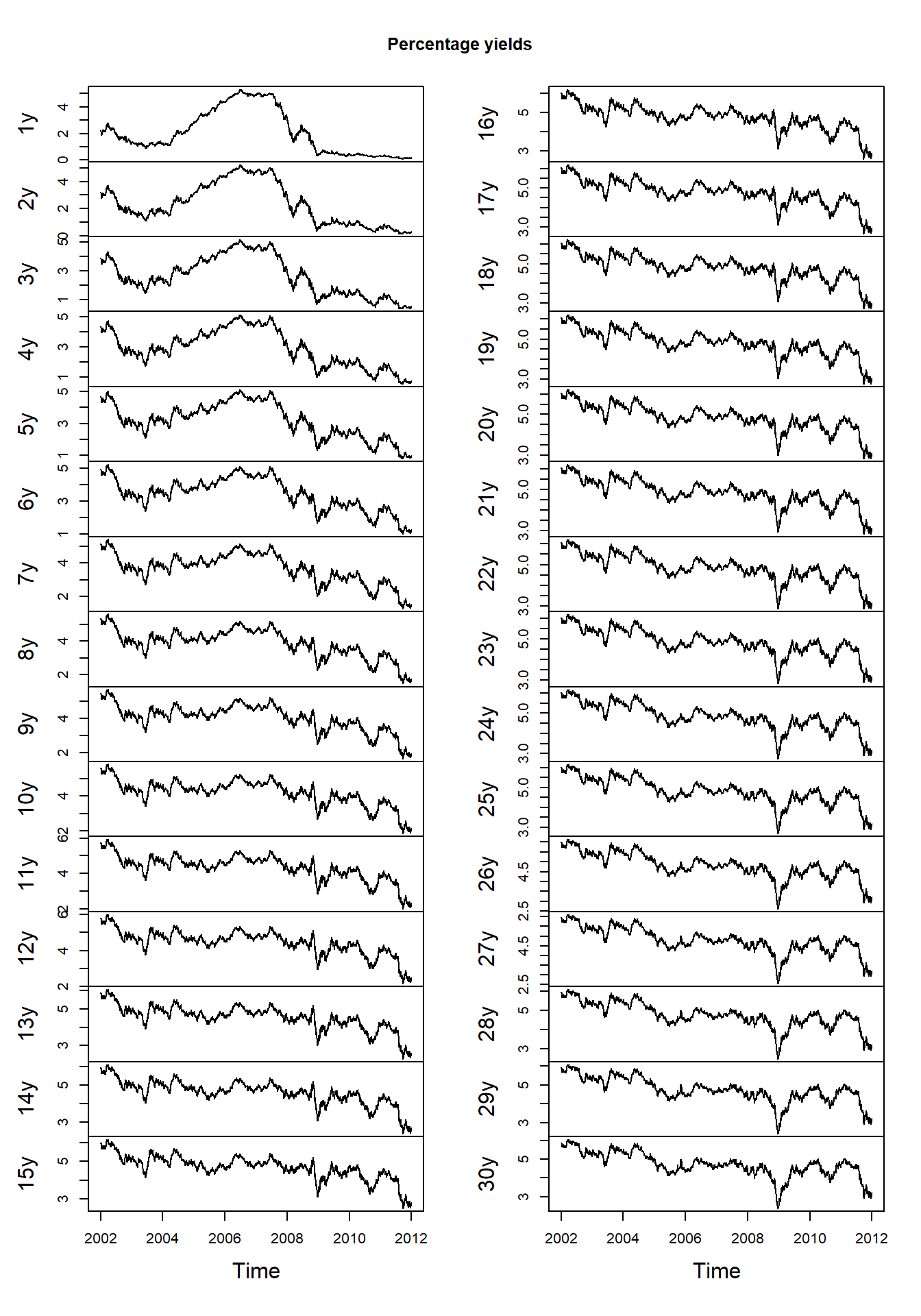
Compute differences (first row is removed):
X = returns(ZCB, method = "diff")Pick 3 maturities:
X3 = X[, c(1, 5, 30)]
plot.zoo(X3, xlab = "Time", main = "Differences (3 maturities)")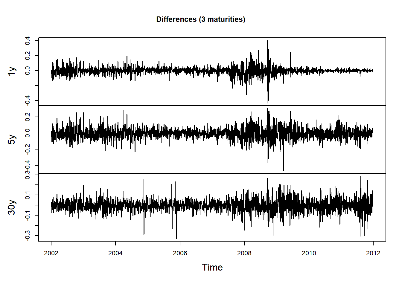
pairs(as.zoo(X3), gap = 0, cex = 0.4)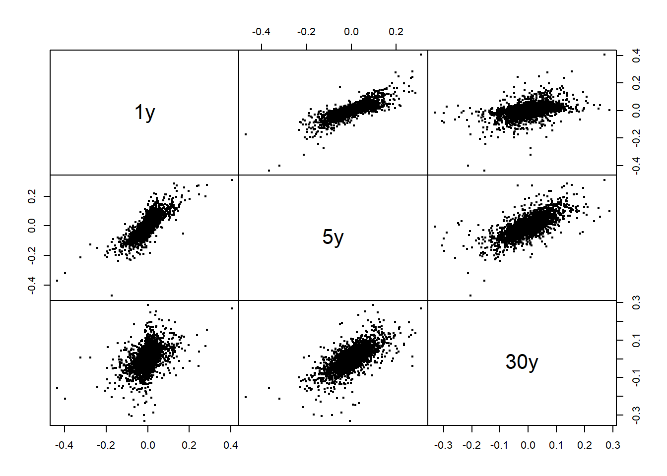
Plot the corresponding “pseudo-observations” (componentwise scaled ranks):
U3 = apply(X3, 2, rank) / (ncol(X3) + 1)
pairs(as.zoo(U3), gap = 0, cex = 0.4)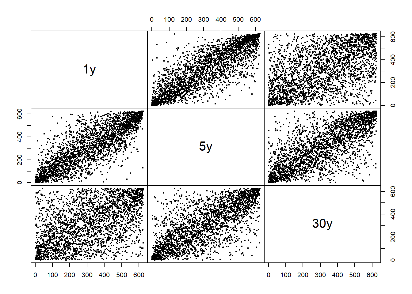
## Note: More on that ("pseudo-observations") in Chapter 73.2 Ljung-Box test of serial independence
Ljung-Box tests of independence.
library(xts)
library(qrmdata)
library(qrmtools)
3.2.1 Constituent data
Dow Jones constituent data:
data("DJ_const")We extract a time period and remove the time series ‘Visa’ (as it only has a very short history in the index):
DJdata = DJ_const['2006-12-29/2015-12-31',-which(names(DJ_const) == "V")]Use plot for zoo objects to get multiple plots:
plot.zoo(DJdata, xlab = "Time", main = "DJ component series (without Visa)")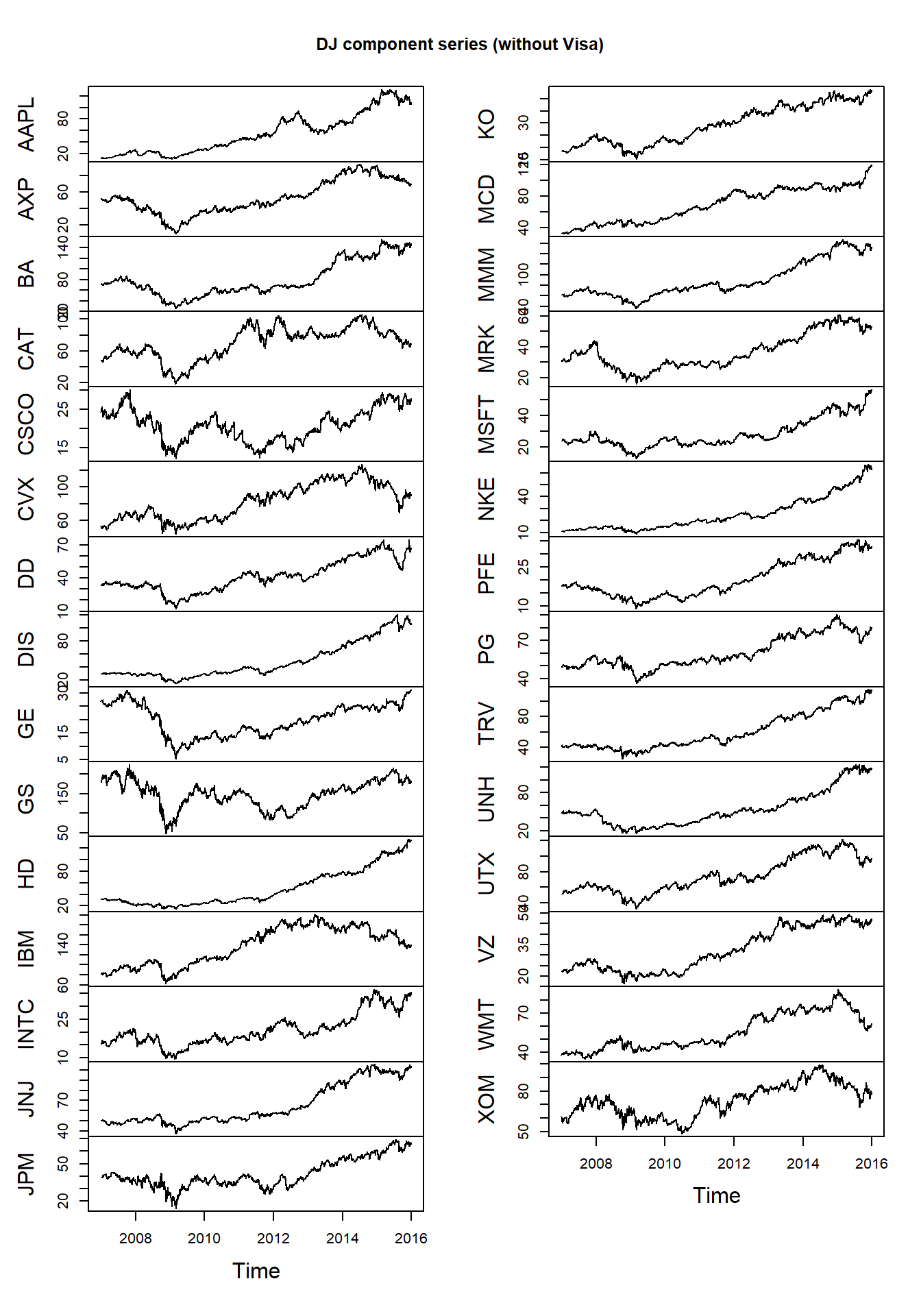
Build log-returns and aggregate to obtain monthly log-returns:
X = returns(DJdata) # could also work with negative log-returns
X.m = apply.monthly(X, FUN = colSums)
3.2.2 Ljung-Box tests of serial independence of stationary data
Compute (lists of) Ljung-Box tests:
\(H_0\): The data are independently distributed.
\(H_1\): The data are not independently distributed; they exhibit serial correlation.
LB.raw   = apply(X,        2, Box.test, lag = 10, type = "Ljung-Box")
LB.abs   = apply(abs(X),   2, Box.test, lag = 10, type = "Ljung-Box") # could also work with squared log-returns
LB.raw.m = apply(X.m,      2, Box.test, lag = 10, type = "Ljung-Box")
LB.abs.m = apply(abs(X.m), 2, Box.test, lag = 10, type = "Ljung-Box")
Extract p-values:
sapplyis likelapply, but returning a vector or matrix instead of a list. Here[[is an extract function which gives a value, e.g.LB.raw[["AAPL"]][["p.value"]].
p.LB.raw   = sapply(LB.raw,   `[[`, "p.value")
p.LB.abs   = sapply(LB.abs,   `[[`, "p.value")
p.LB.raw.m = sapply(LB.raw.m, `[[`, "p.value")
p.LB.abs.m = sapply(LB.abs.m, `[[`, "p.value")
round(cbind(p.LB.raw, p.LB.abs, p.LB.raw.m, p.LB.abs.m), 2)
## p.LB.raw p.LB.abs p.LB.raw.m p.LB.abs.m
## AAPL 0.14 0 0.54 0.00
## AXP 0.00 0 0.01 0.00
## BA 0.03 0 0.13 0.00
## CAT 0.08 0 0.01 0.00
## CSCO 0.11 0 0.32 0.14
## CVX 0.00 0 0.60 0.30
## DD 0.00 0 0.09 0.02
## DIS 0.00 0 0.00 0.04
## GE 0.00 0 0.17 0.00
## GS 0.00 0 0.61 0.00
## HD 0.25 0 0.12 0.42
## IBM 0.00 0 0.67 0.64
## INTC 0.00 0 0.65 0.90
## JNJ 0.00 0 0.25 0.30
## JPM 0.00 0 0.62 0.00
## KO 0.00 0 0.01 0.22
## MCD 0.00 0 0.10 0.60
## MMM 0.00 0 0.36 0.51
## MRK 0.03 0 0.45 0.01
## MSFT 0.00 0 0.80 0.90
## NKE 0.00 0 0.79 0.73
## PFE 0.00 0 0.32 0.05
## PG 0.00 0 0.78 0.04
## TRV 0.00 0 0.30 0.81
## UNH 0.00 0 0.03 0.00
## UTX 0.00 0 0.02 0.08
## VZ 0.00 0 0.10 0.43
## WMT 0.00 0 0.83 0.86
## XOM 0.00 0 0.60 0.403.2.3 Reproduce Ljung-Box tests from the QRM book
Up to minor differences (see below), this reproduces Table 3.1 in the MFE (2015):
## Note: This uses older DJ data from 'QRM' package
DJ.QRM = QRM::DJ
DJ.old = as.xts(DJ.QRM)
DJ.old = DJ.old['1993-01-01/2000-12-31']
X.old = returns(DJ.old)
X.old.m = apply.monthly(X.old, FUN = colSums)
Compute (lists of) Ljung-Box tests:
LB.raw   = apply(X.old,        2, Box.test, lag = 10, type = "Ljung-Box")
LB.abs   = apply(abs(X.old),   2, Box.test, lag = 10, type = "Ljung-Box")
LB.raw.m = apply(X.old.m,      2, Box.test, lag = 10, type = "Ljung-Box")
LB.abs.m = apply(abs(X.old.m), 2, Box.test, lag = 10, type = "Ljung-Box")
Extract p-values:
p.LB.raw   = sapply(LB.raw,   `[[`, "p.value")
p.LB.abs   = sapply(LB.abs,   `[[`, "p.value")
p.LB.raw.m = sapply(LB.raw.m, `[[`, "p.value")
p.LB.abs.m = sapply(LB.abs.m, `[[`, "p.value")
(res = round(cbind(p.LB.raw, p.LB.abs, p.LB.raw.m, p.LB.abs.m), 2))
## p.LB.raw p.LB.abs p.LB.raw.m p.LB.abs.m
## AA 0.00 0 0.23 0.02
## AXP 0.02 0 0.54 0.07
## T 0.11 0 0.70 0.02
## BA 0.03 0 0.90 0.15
## CAT 0.28 0 0.73 0.07
## C 0.09 0 0.91 0.49
## KO 0.00 0 0.50 0.03
## DD 0.03 0 0.74 0.00
## EK 0.15 0 0.59 0.54
## XOM 0.00 0 0.33 0.22
## GE 0.00 0 0.25 0.09
## GM 0.64 0 0.82 0.26
## HWP 0.10 0 0.21 0.02
## HD 0.00 0 0.00 0.41
## HON 0.44 0 0.07 0.30
## INTC 0.23 0 0.80 0.62
## IBM 0.18 0 0.67 0.27
## IP 0.15 0 0.01 0.09
## JPM 0.52 0 0.43 0.12
## JNJ 0.00 0 0.10 0.89
## MCD 0.28 0 0.72 0.67
## MRK 0.05 0 0.54 0.65
## MSFT 0.28 0 0.19 0.13
## MMM 0.00 0 0.57 0.33
## MO 0.01 0 0.69 0.82
## PG 0.02 0 0.99 0.73
## SBC 0.05 0 0.12 0.00
## UTX 0.00 0 0.12 0.01
## WMT 0.00 0 0.42 0.63
## DIS 0.44 0 0.01 0.52Note: The minor differences to the tables in the book come from a different approach. The tables in the book were produces without ‘xts’ objects:
library(timeSeries) # Caution: returns() now from timeSeries## Loading required package: timeDate##
## Attaching package: 'timeSeries'## The following object is masked from 'package:zoo':
##
## time<-## The following object is masked from 'package:qrmtools':
##
## returnsX.old. = returns(DJ.QRM)
X.old. = window(X.old., start = timeDate("1993-01-01"), end = timeDate("2000-12-31"))
X.old.m. = aggregate(X.old., by = unique(timeLastDayInMonth(time(X.old.))), sum)
detach("package:timeSeries")Compute (lists of) Ljung-Box tests:
LB.raw.   = apply(X.old.,        2, Box.test, lag = 10, type = "Ljung-Box")
LB.abs.   = apply(abs(X.old.),   2, Box.test, lag = 10, type = "Ljung-Box")
LB.raw.m. = apply(X.old.m.,      2, Box.test, lag = 10, type = "Ljung-Box")
LB.abs.m. = apply(abs(X.old.m.), 2, Box.test, lag = 10, type = "Ljung-Box")
Extract p-values:
p.LB.raw.   = sapply(LB.raw.,   `[[`, "p.value")
p.LB.abs.   = sapply(LB.abs.,   `[[`, "p.value")
p.LB.raw.m. = sapply(LB.raw.m., `[[`, "p.value")
p.LB.abs.m. = sapply(LB.abs.m., `[[`, "p.value")
Result:
(res. = round(cbind(p.LB.raw., p.LB.abs., p.LB.raw.m., p.LB.abs.m.), 2))## p.LB.raw. p.LB.abs. p.LB.raw.m. p.LB.abs.m.
## AA 0.00 0 0.23 0.02
## AXP 0.02 0 0.55 0.07
## T 0.11 0 0.70 0.02
## BA 0.03 0 0.90 0.17
## CAT 0.28 0 0.73 0.07
## C 0.09 0 0.91 0.48
## KO 0.00 0 0.50 0.03
## DD 0.03 0 0.75 0.00
## EK 0.15 0 0.61 0.54
## XOM 0.00 0 0.32 0.22
## GE 0.00 0 0.25 0.09
## GM 0.65 0 0.81 0.27
## HWP 0.09 0 0.21 0.02
## HD 0.00 0 0.00 0.41
## HON 0.44 0 0.07 0.30
## INTC 0.23 0 0.79 0.62
## IBM 0.18 0 0.67 0.28
## IP 0.15 0 0.01 0.09
## JPM 0.52 0 0.43 0.12
## JNJ 0.00 0 0.11 0.91
## MCD 0.28 0 0.72 0.68
## MRK 0.05 0 0.53 0.65
## MSFT 0.28 0 0.19 0.13
## MMM 0.00 0 0.57 0.33
## MO 0.01 0 0.68 0.82
## PG 0.02 0 0.99 0.74
## SBC 0.05 0 0.13 0.00
## UTX 0.00 0 0.12 0.01
## WMT 0.00 0 0.41 0.64
## DIS 0.44 0 0.01 0.51Differences:
summary(res-res.)## p.LB.raw p.LB.abs p.LB.raw.m p.LB.abs.m
## Min. :-0.01 Min. :0 Min. :-0.02 Min. :-0.020000000
## 1st Qu.: 0.00 1st Qu.:0 1st Qu.: 0.00 1st Qu.: 0.000000000
## Median : 0.00 Median :0 Median : 0.00 Median : 0.000000000
## Mean : 0.00 Mean :0 Mean : 0.00 Mean :-0.002333333
## 3rd Qu.: 0.00 3rd Qu.:0 3rd Qu.: 0.00 3rd Qu.: 0.000000000
## Max. : 0.01 Max. :0 Max. : 0.01 Max. : 0.0100000003.3 Univariate stylized facts
Illustrates univariate stylized facts for financial return series.
Univariate stylized facts:
(U1) Return series are not iid although they show little serial correlation;
(U2) Series of absolute (or squared) returns show profound serial correlation;
(U3) Conditional expected returns are close to zero;
(U4) Volatility (conditional standard deviation) appears to vary over time;
(U5) Extreme returns appear in clusters;
(U6) Return series are leptokurtic or heavy-tailed (power-like tail).
library(xts)
library(qrmdata)
library(qrmtools)
3.3.1 Index data
data("SP500")
data("FTSE")
data("SMI")
Build log-returns:
SP500.X = returns(SP500)
FTSE.X = returns(FTSE)
SMI.X = returns(SMI)
Remove zero returns (caused almost certainly by market closure):
SP500.X = SP500.X[SP500.X != 0]
SMI.X = SMI.X[SMI.X != 0]
FTSE.X = FTSE.X[FTSE.X != 0]
Merge and aggregate:
X = merge(SP500 = SP500.X, FTSE = FTSE.X, SMI = SMI.X, all = FALSE)
X.w = apply.weekly(X, FUN = colSums) # weekly log-returns (summing within weeks)
3.3.2 (U1) and (U2)
(U1) Return series are not iid although they show little serial correlation
(U2) Series of absolute (or squared) returns show profound serial correlation
Auto- and crosscorrelations of returns and absolute returns:
acf(X)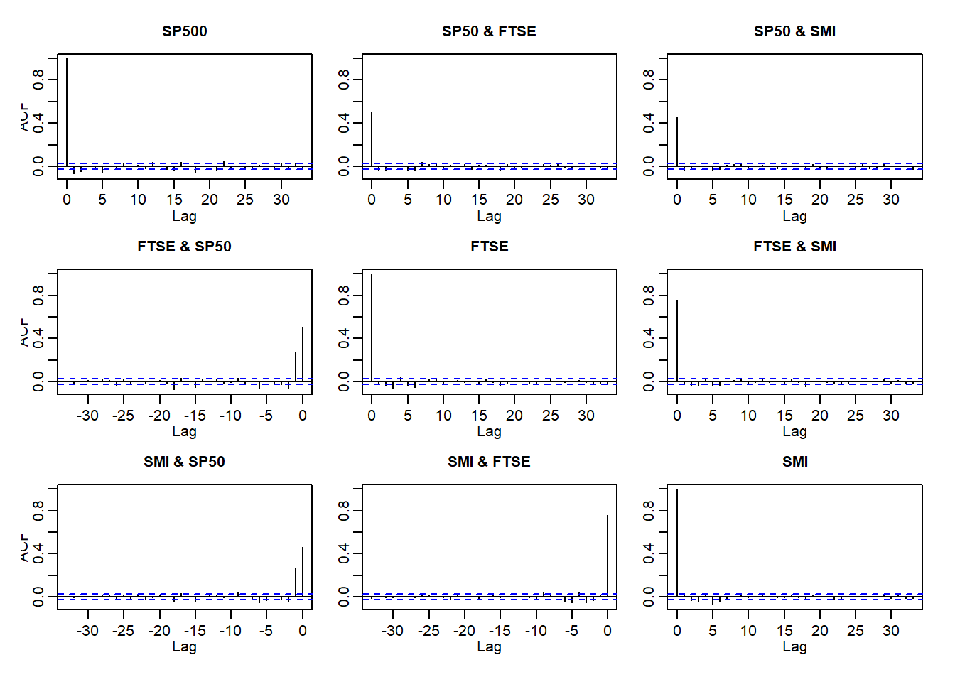
acf(abs(X))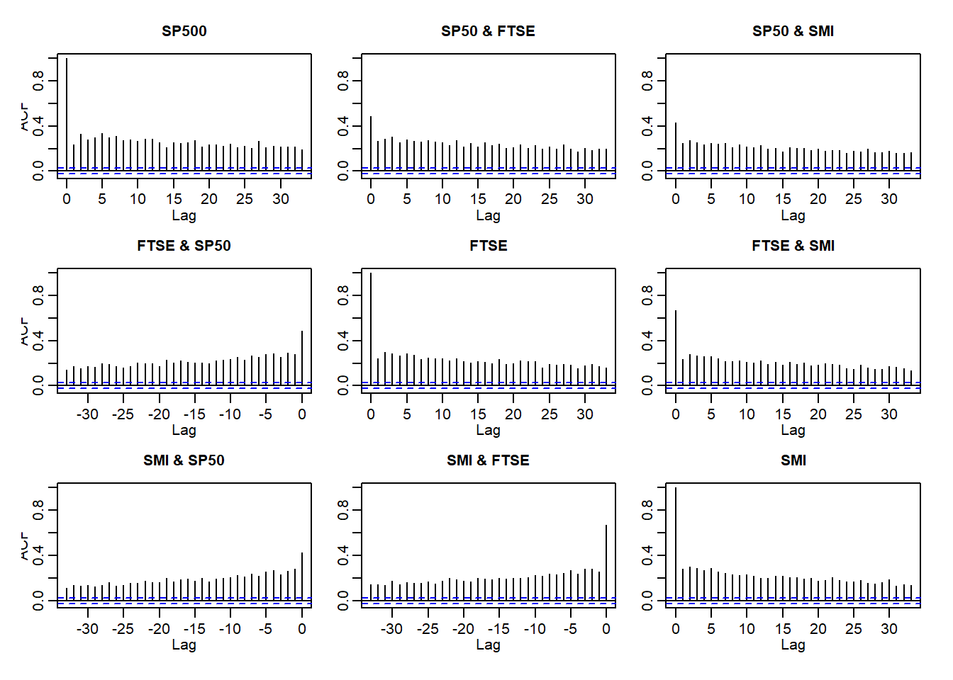
acf(X.w)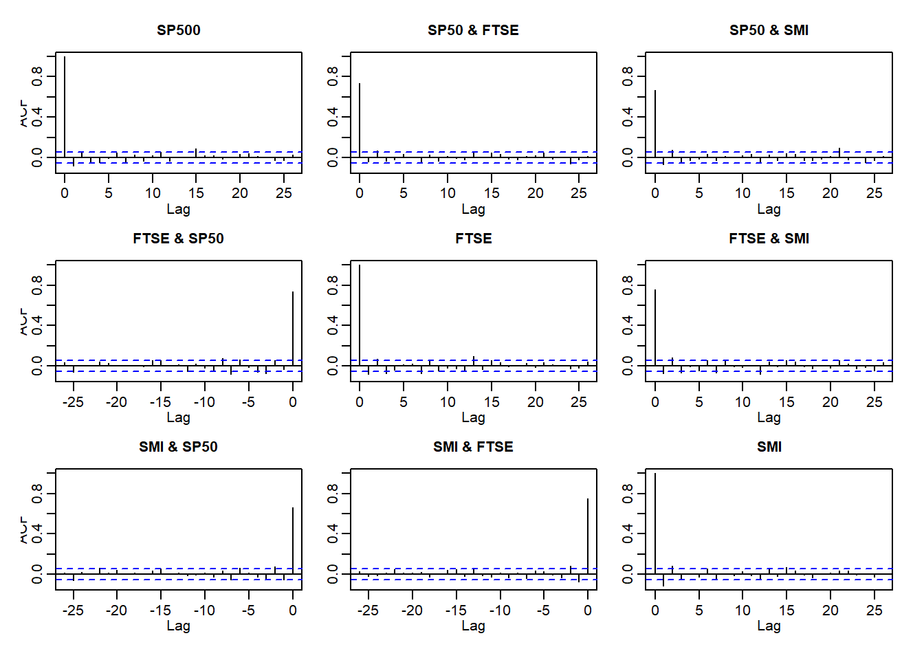
acf(abs(X.w))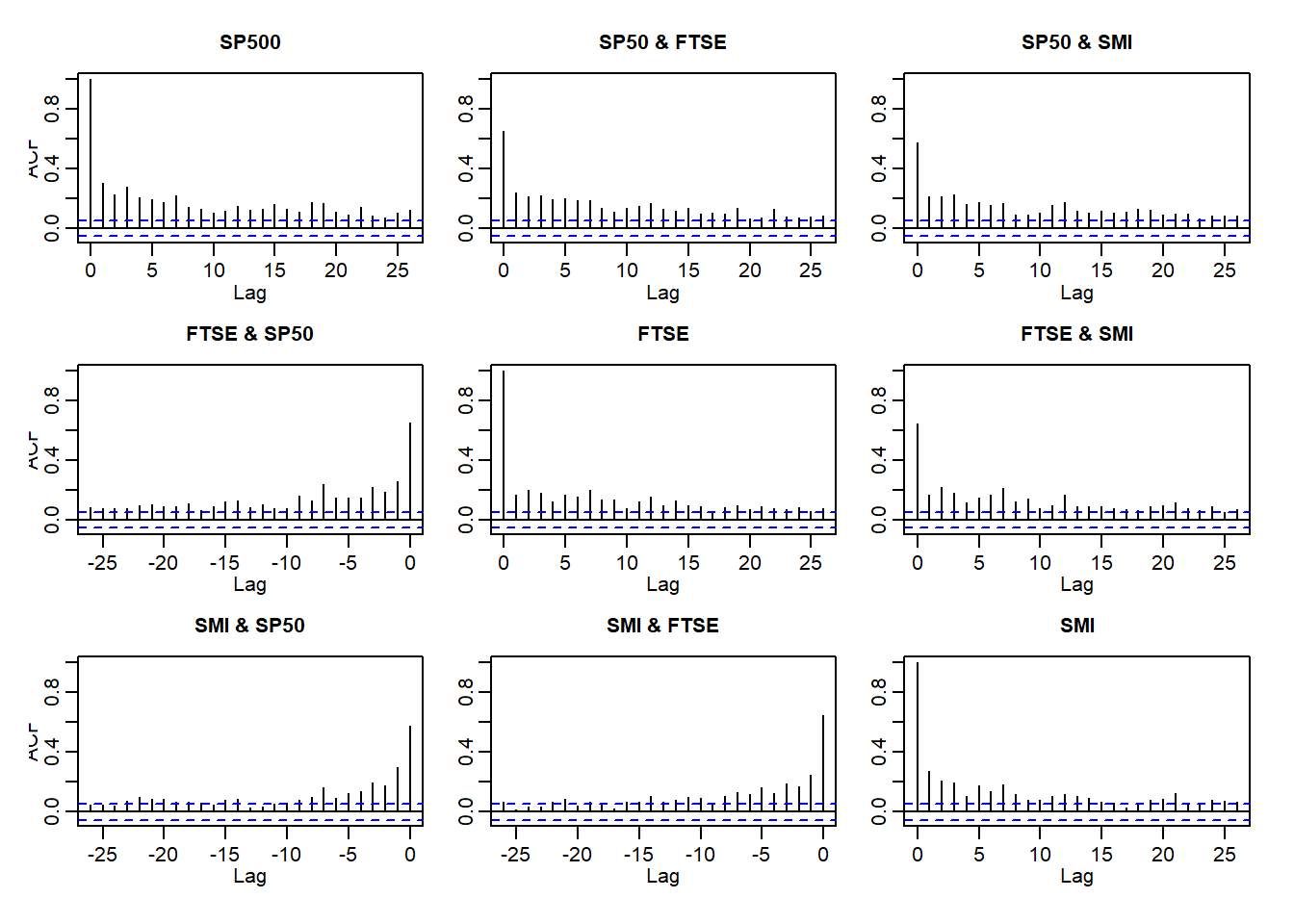
3.3.3 (U3) and (U4)
(U3) Conditional expected returns are close to zero;
(U4) Volatility (conditional standard deviation) appears to vary over time;
Plot of returns:
plot.zoo(X, xlab = "Time", main = "Log-returns") # this (partly) confirms (U3)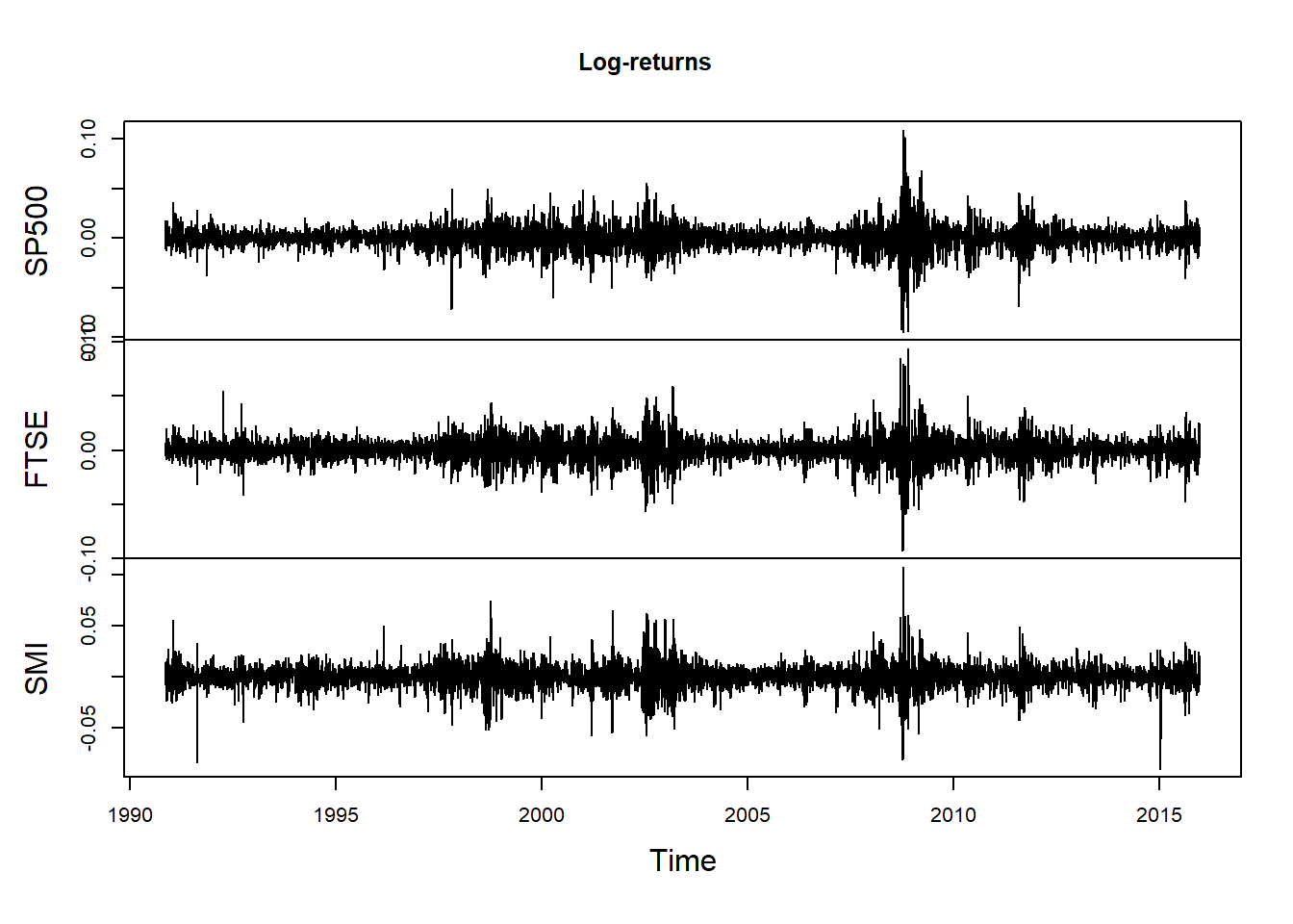
Plot of volatilities:
X.vols = apply.monthly(X, FUN = function(x) apply(x, 2, sd)) # componentwise volatilities
plot.zoo(X.vols, xlab = "Time", main = "Volatility estimates")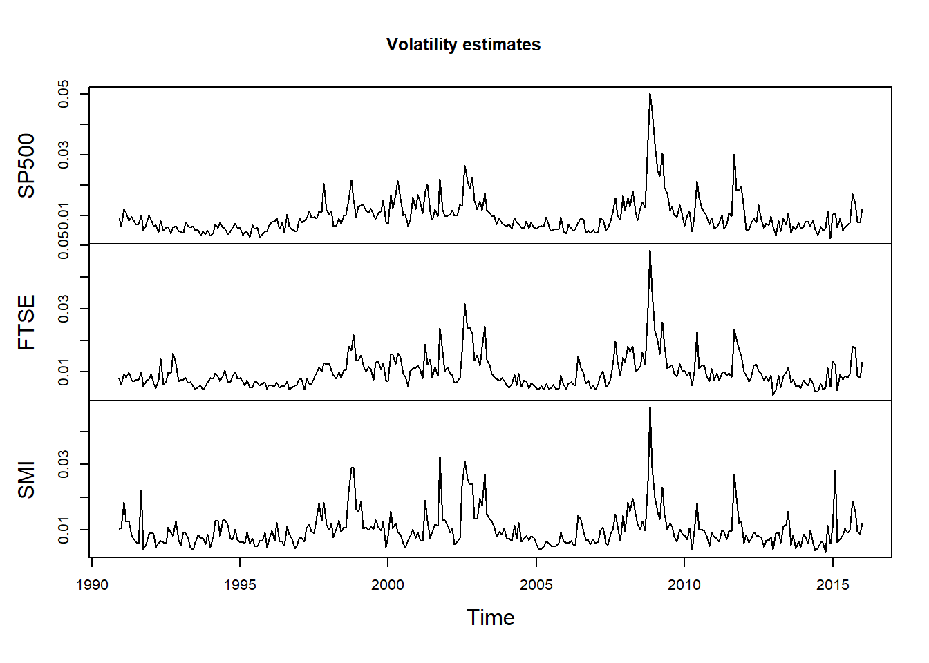
3.3.4 (U5)
- (U5) Extreme returns appear in clusters
Plot the largest losses (already partly confirms (U5)):
L = -SP500.X # consider -log-returns of S&P 500 here
r = 0.01 # probability to determine large losses
u = quantile(L, probs = 1 - r) # determine empirical (1-r)-quantile
xtr.L = L[L > u] # exceedances over the chosen empirical quantile = largest so-many losses
plot(as.numeric(xtr.L), type = "h", xlab = "Time",
     ylab = substitute("Largest"~r.*"% of losses ("*n.~"losses)",
                       list(r. = 100 * r, n. = length(xtr.L))))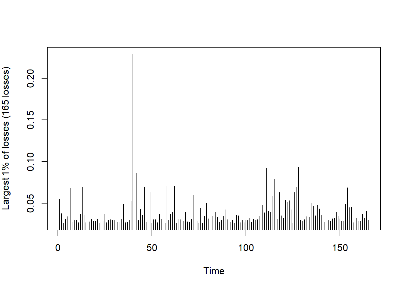
Now consider spacings (certainly not exponentially distributed):
spcs = as.numeric(diff(time(xtr.L)))
qq_plot(spcs, FUN = function(p) qexp(p, rate = r)) # r = exceedance probability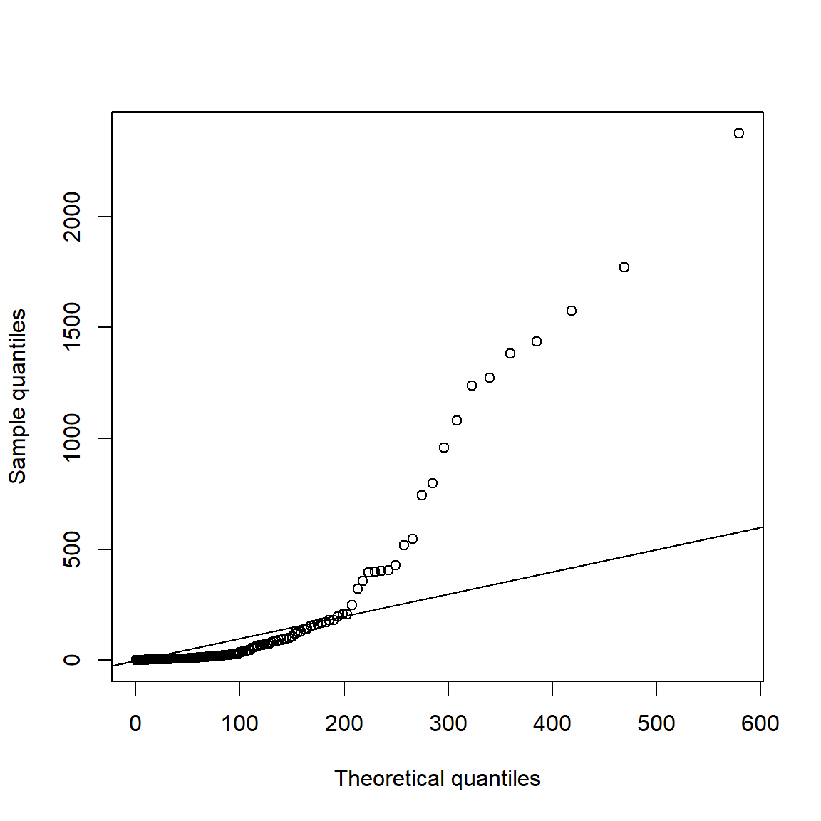
Compare with a Poisson process (simulated iid data):
set.seed(271)
L. = rt(length(L), df = 3) # simulate iid data from a t_3 distribution
u. = quantile(L., probs = 1 - r) # determine empirical (1-r)-quantile
xtr.L. = L.[L. > u.] # exceedances
plot(xtr.L., type = "h", xlab = "Time",
     ylab = substitute("Largest"~r.*"% of losses ("*n.~"losses)",
                       list(r. = 100 * r, n. = length(xtr.L.))))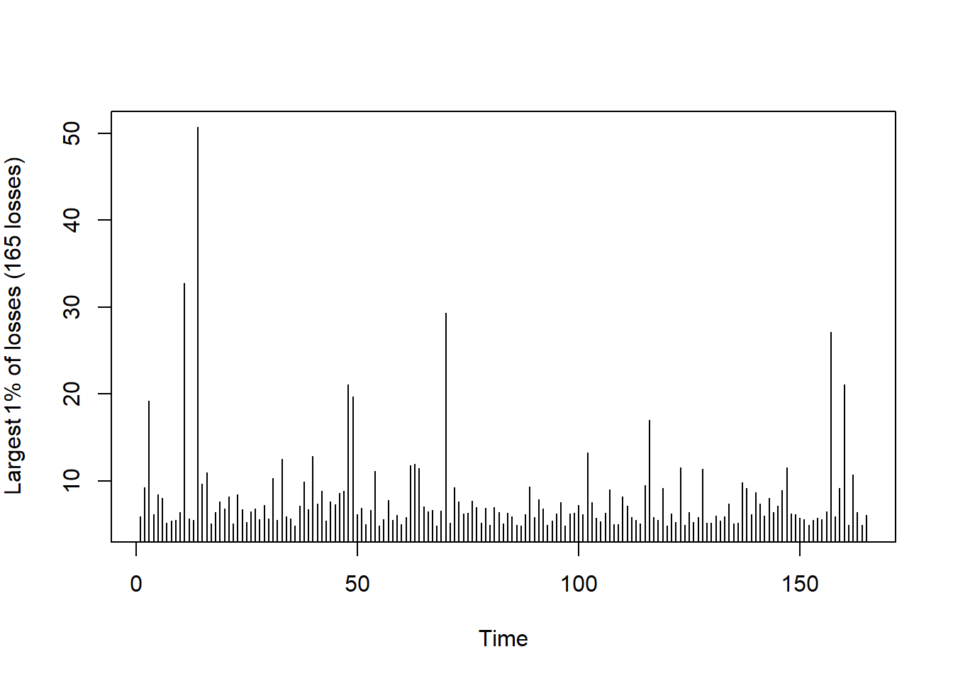
Sapcings:
spcs. = diff(which(L. > u.))
qq_plot(spcs., FUN = function(p) qexp(p, rate = r))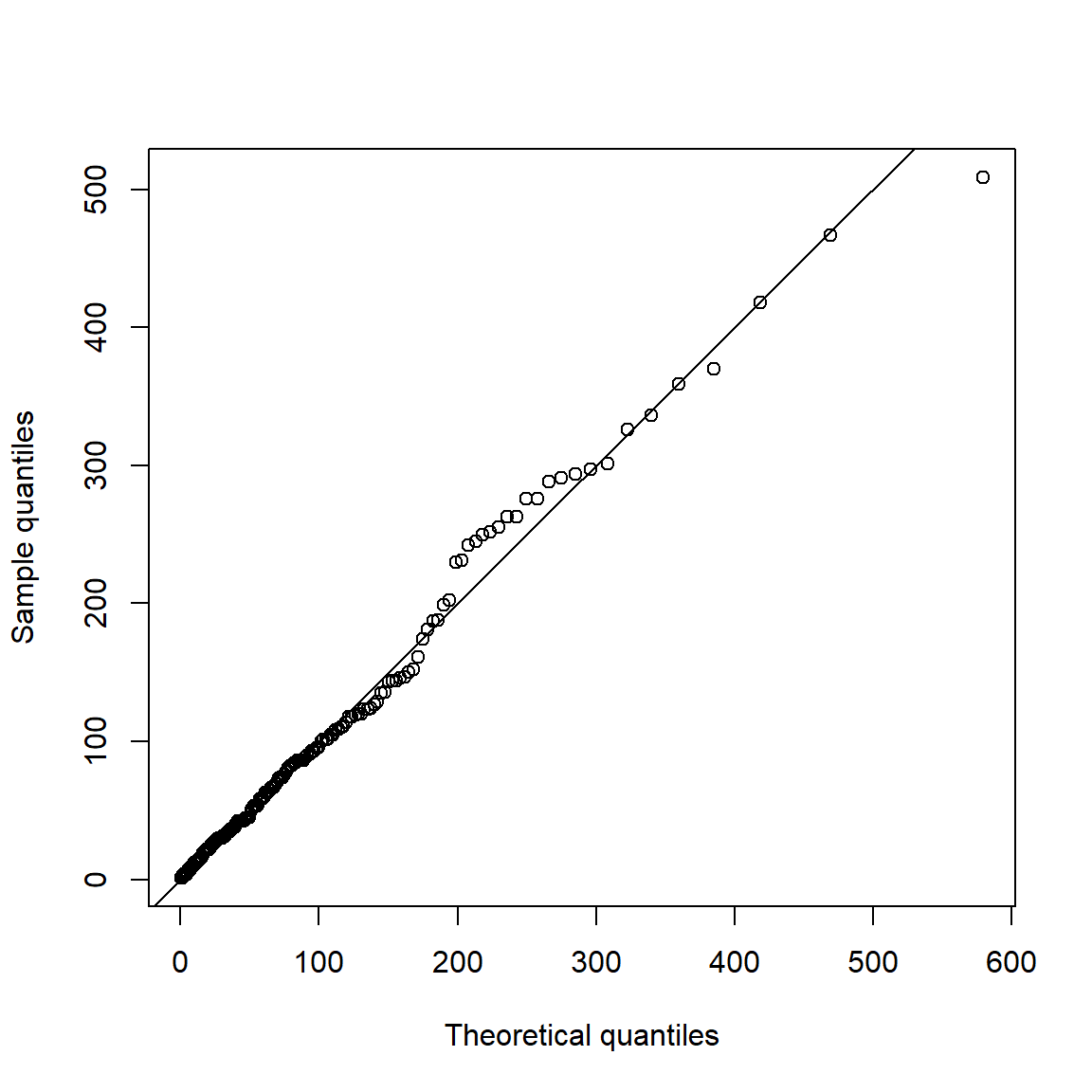
3.3.5 (U6)
- (U6) Return series are leptokurtic or heavy-tailed (power-like tail)
Show leptokurtosis (heavier tails than a normal) by Q-Q plots against a normal:
layout(t(1:3)) # (1,3)-layout
for (i in 1:3)
    qq_plot(X.w[,i], FUN = qnorm, method = "empirical",
            # ... to account for the unknown location (mu) and scale (sig) of qnorm()
            main = names(X.w)[i]) # equivalent to qqnorm(); qqline()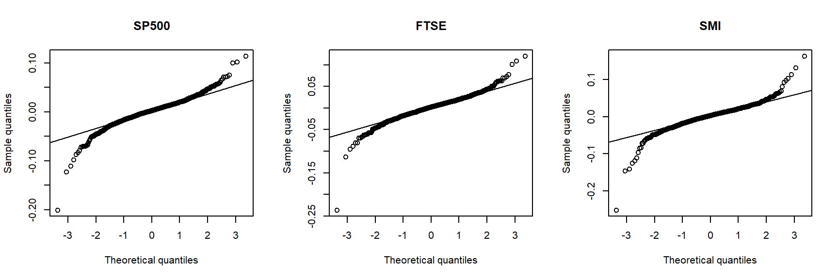
layout(1) # restore layout
## One can also look at various formal tests
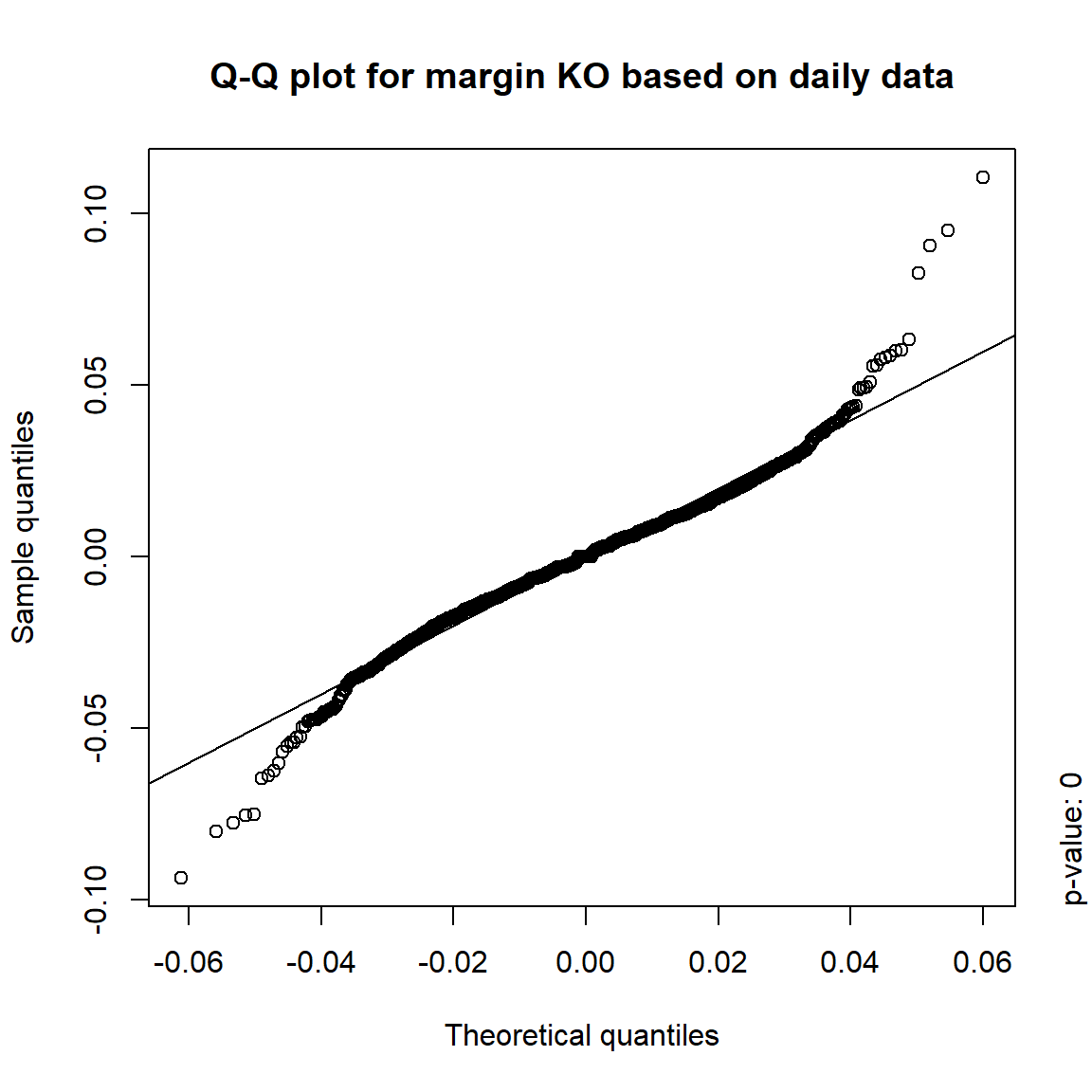
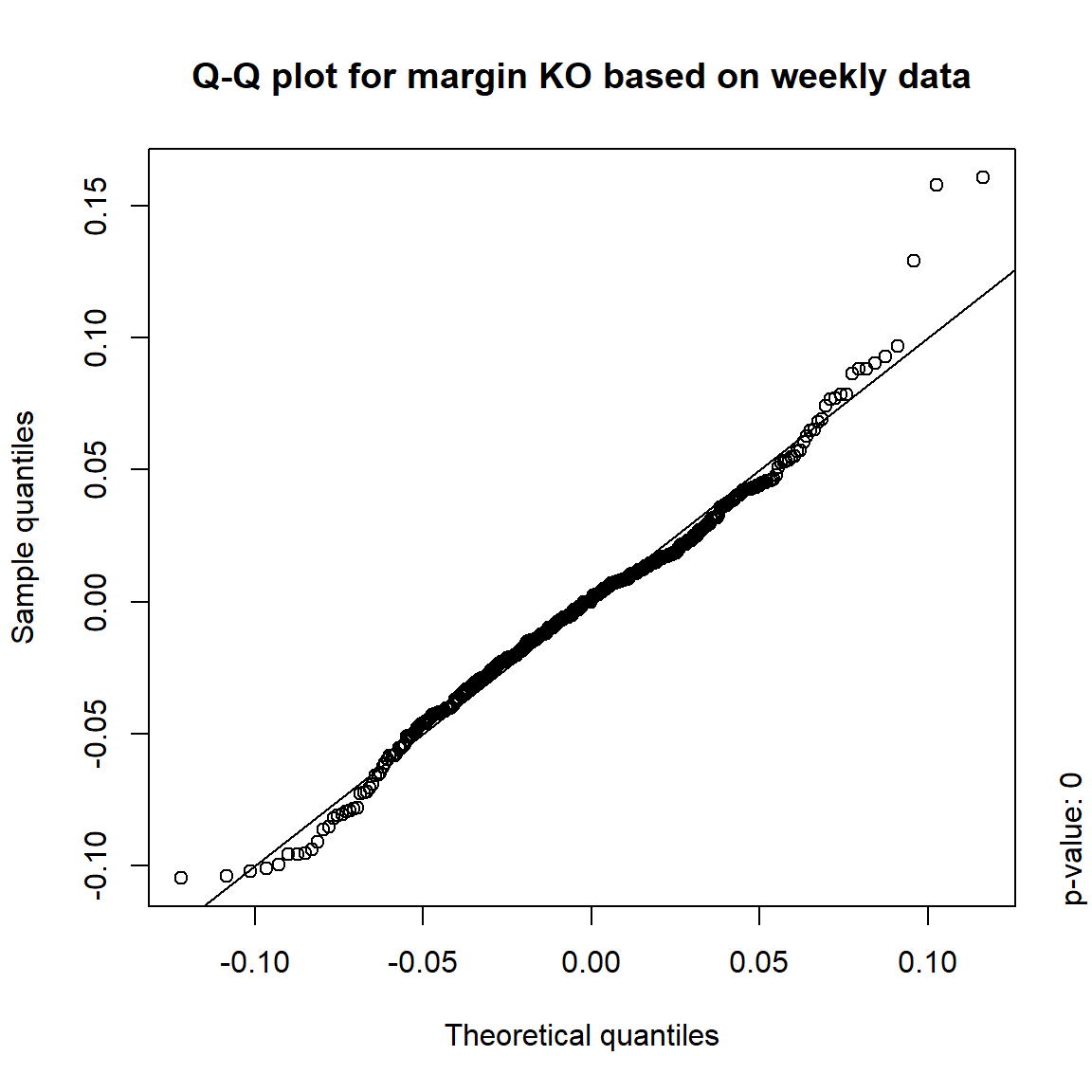
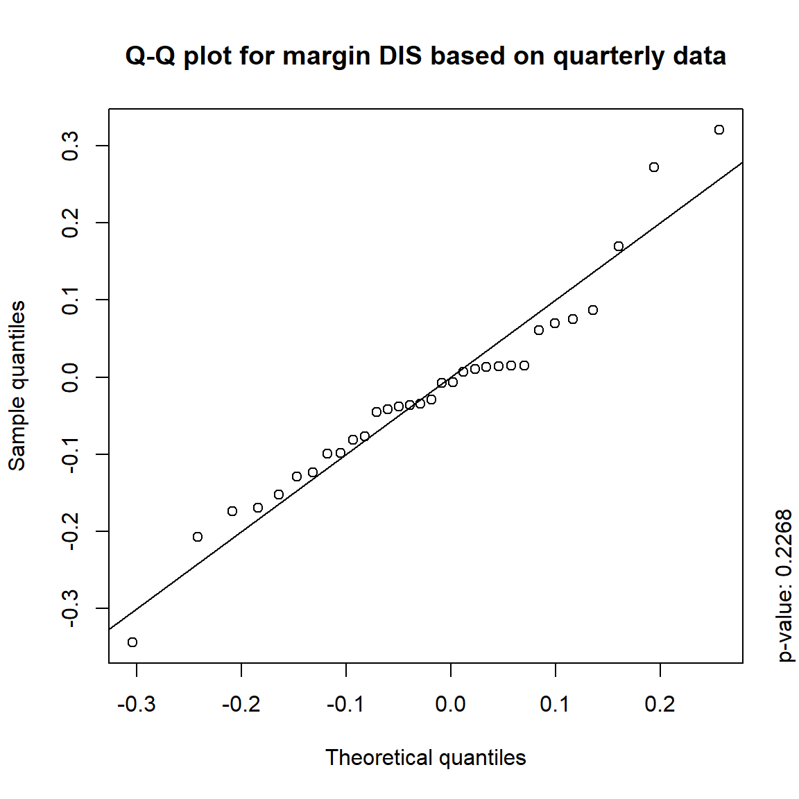
A Q–Q plot (quantile–quantile plot) is a standard visual tool for showing the relationship between empirical quantiles of the data and theoretical quantiles of a reference distribution. A lack of linearity in the Q–Q plot is interpreted as evidence against the hypothesized reference distribution.
The inverted S-shaped curve of the points suggests that the more extreme empirical quantiles of the data tend to be larger than the corresponding quantiles of a normal distribution, indicating that the normal distribution is a poor model for these returns.
3.4 Testing univariate normality
Univariate tests of normality, data application and uniformity of p-values.
library(nortest) # for cvm.test()
library(ADGofTest) # for ad.test()
##
## Attaching package: 'ADGofTest'## The following object is masked from 'package:nortest':
##
## ad.testlibrary(moments) # for agostino.test(), jarque.test()##
## Attaching package: 'moments'## The following objects are masked from 'package:timeDate':
##
## kurtosis, skewnesslibrary(xts) # for time-series related functions
library(qrmdata)
library(qrmtools)3.4.1 Generate data
n = 1000 # sample size
mu = 1 # location
sig = 2 # scale
nu = 3 # degrees of freedom
set.seed(271) # set seed (for reproducibility)
X.N = rnorm(n, mean = mu, sd = sig) # sample from N(mu, sig^2)
X.t = mu + sig * rt(n, df = nu) * sqrt((nu-2)/nu) # sample from t_nu(mu, sqrt((nu-2)/nu)*sig^2) (also variance sig^2)
if(FALSE) {
    var(X.N)
    var(X.t)
    ## => quite apart, but closer for larger n
}
3.4.2 Testing for \(\mathcal{N}(\mu, \sigma^2)\)
We treat \(\mu\) and \(\sigma^2\) as unknown and estimate them:
mu.N = mean(X.N)
mu.t = mean(X.t)
sig.N = sd(X.N)
sig.t = sd(X.t)
Tests for general distributions (here applied to the normal)
The Kolmogorov–Smirnov test:
is a nonparametric test of the equality of continuous, one-dimensional probability distributions that can be used to compare a sample with a reference probability distribution (one-sample K–S test), or to compare two samples (two-sample K–S test).
can be modified to serve as a goodness of fit test. In the special case of testing for normality of the distribution.
\(H_0\): the distribution function which generated \(X\) is normal distribution with specified parameters.
The Cramer-von Mises test
is an EDF omnibus test for the composite hypothesis of normality.
\(H_0\): the distribution function which generated \(X\) is normal.
The Anderson-Darling goodness of fit test:
checks whether \(X\) is a iid sample from the distribution described by such CDF.
\(H_0\): the distribution function which generated \(X\) is normal distribution with specified parameters.
Applied to normal data (with estimated \(\mu\) and \(\sigma^2\)):
(ks = ks.test(X.N, y = "pnorm", mean = mu.N, sd = sig.N)) # Kolmogorov--Smirnov##
## One-sample Kolmogorov-Smirnov test
##
## data: X.N
## D = 0.023172117, p-value = 0.6562203
## alternative hypothesis: two-sided(cvm = cvm.test(X.N)) # Cramer--von Mises for normality##
## Cramer-von Mises normality test
##
## data: X.N
## W = 0.053604764, p-value = 0.4591003(ad = ad.test(X.N, distr.fun = pnorm, mean = mu.N, sd = sig.N)) # Anderson--Darling##
## Anderson-Darling GoF Test
##
## data: X.N and pnorm
## AD = 0.34126087, p-value = 0.9042402
## alternative hypothesis: NAstopifnot(min(ks$p.value, cvm$p.value, ad$p.value) >= 0.05) # => no rejectionsApplied to \(t\) data (with estimated \(\mu\) and \(\sigma^2\)):
(ks = ks.test(X.t, y = "pnorm", mean = mu.t, sd = sig.t)) # Kolmogorov--Smirnov##
## One-sample Kolmogorov-Smirnov test
##
## data: X.t
## D = 0.14299637, p-value < 2.2204e-16
## alternative hypothesis: two-sided(cvm = cvm.test(X.t)) # Cramer--von Mises for normality## Warning in cvm.test(X.t): p-value is smaller than 7.37e-10, cannot be computed
## more accurately##
## Cramer-von Mises normality test
##
## data: X.t
## W = 8.0937659, p-value = 7.37e-10(ad = ad.test(X.t, distr.fun = pnorm, mean = mu.t, sd = sig.t)) # Anderson--Darling##
## Anderson-Darling GoF Test
##
## data: X.t and pnorm
## AD = Inf, p-value = 6e-07
## alternative hypothesis: NAstopifnot(max(ks$p.value, cvm$p.value, ad$p.value) < 0.05) # => all rejections based on 5%Tests specifically for the normal distribution
The Shapiro-Wilk test of normality:
- \(H_0\): the distribution function which generated \(X\) is normal.
D’Agostino test for skewness:
Under the hypothesis of normality, data should be symmetrical (i.e. skewness should be equal to zero). This test has such null hypothesis and is useful to detect a significant skewness in normally distributed data.
\(H_0\): data have no skewness.
The Jarque-Bera test for normality:
Under the hypothesis of normality, data should be symmetrical (i.e. skewness should be equal to zero) and have kurtosis chose to three. The Jarque-Bera statistic is chi-square distributed with two degrees of freedom.
\(H_0\): skewness and excess kurtosis equal 0.
Applied to normal data:
(sh = shapiro.test(X.N)) # Shapiro--Wilk##
## Shapiro-Wilk normality test
##
## data: X.N
## W = 0.99811173, p-value = 0.3326257(ag = agostino.test(X.N)) # D'Agostino's test##
## D'Agostino skewness test
##
## data: X.N
## skew = -0.077540707, z = -1.006945762, p-value = 0.3139608
## alternative hypothesis: data have a skewness(jb = jarque.test(X.N)) # Jarque--Bera test##
## Jarque-Bera Normality Test
##
## data: X.N
## JB = 1.210698, p-value = 0.5458839
## alternative hypothesis: greaterstopifnot(min(sh$p.value, ag$p.value, jb$p.value) >= 0.05) # => no rejectionsApplied to \(t\) data:
(sh = shapiro.test(X.t)) # Shapiro--Wilk##
## Shapiro-Wilk normality test
##
## data: X.t
## W = 0.60189343, p-value < 2.2204e-16(ag = agostino.test(X.t)) # D'Agostino's test##
## D'Agostino skewness test
##
## data: X.t
## skew = -0.61633906, z = -7.41259243, p-value = 1.239009e-13
## alternative hypothesis: data have a skewness(jb = jarque.test(X.t)) # Jarque--Bera test##
## Jarque-Bera Normality Test
##
## data: X.t
## JB = 793183.43, p-value < 2.2204e-16
## alternative hypothesis: greaterstopifnot(max(sh$p.value, ag$p.value, jb$p.value) < 0.05) # => all rejections based on 5%Graphical tests of normality
Note that Q-Q plots are more widely used than P-P plots (probability-probability plots) (as they highlight deviations in the tails more clearly).
Applied to normal data:
pp_plot(X.N, FUN = function(q) pnorm(q, mean = mu.N, sd = sig.N))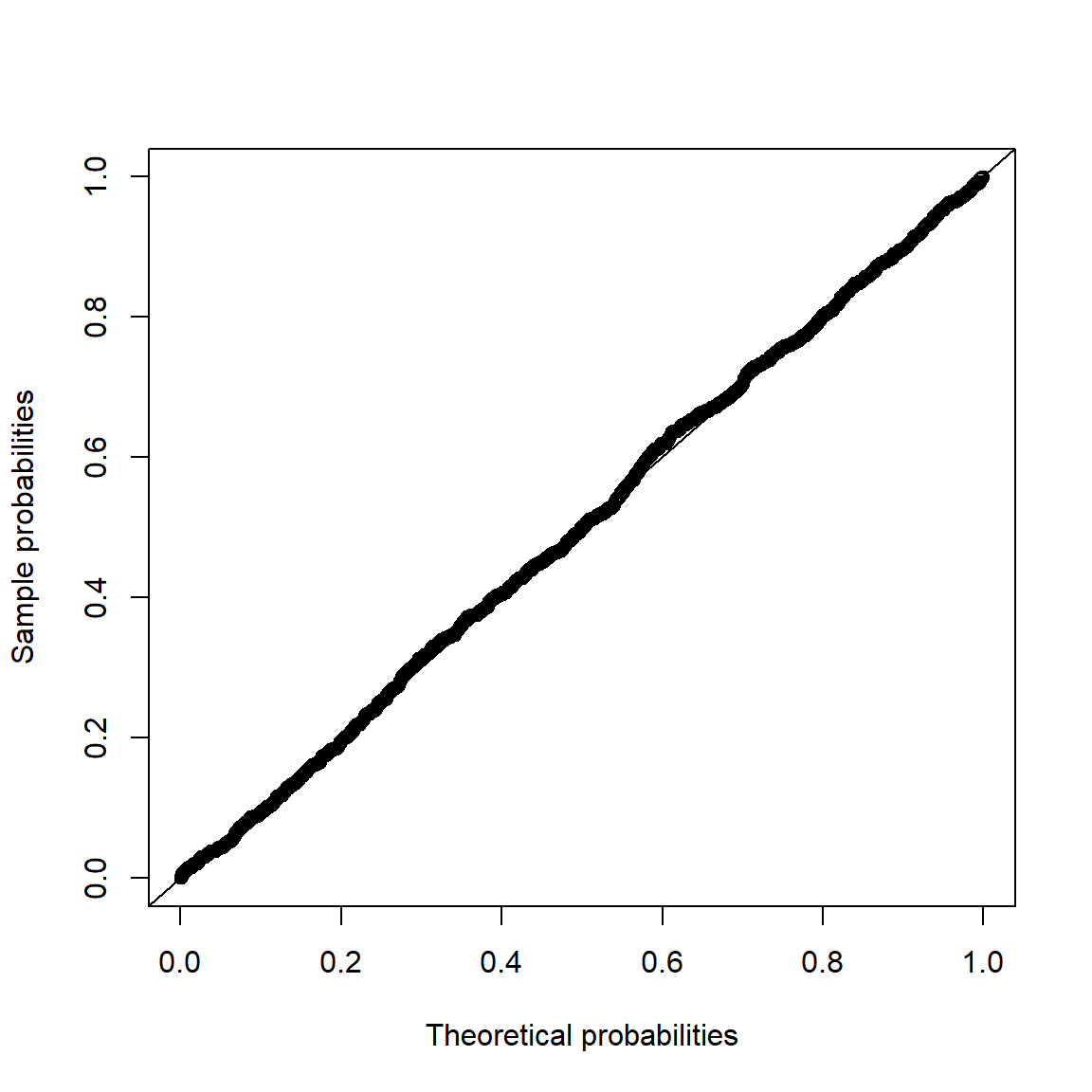
qq_plot(X.N, FUN = function(p) qnorm(p, mean = mu.N, sd = sig.N))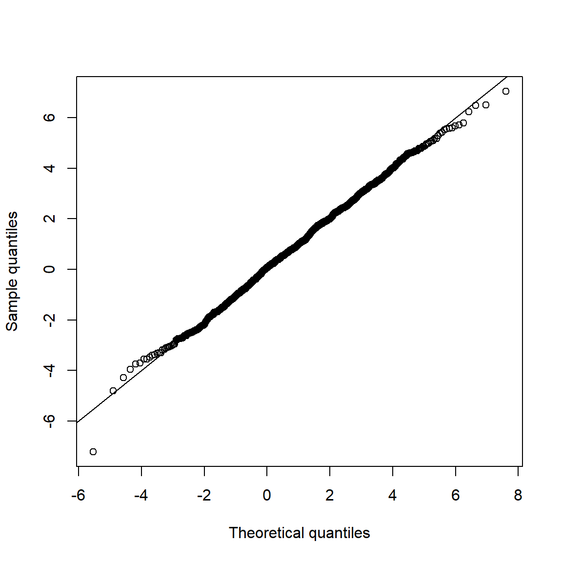
Applied to \(t\) data:
pp_plot(X.t, FUN = function(q) pnorm(q, mean = mu.t, sd = sig.t))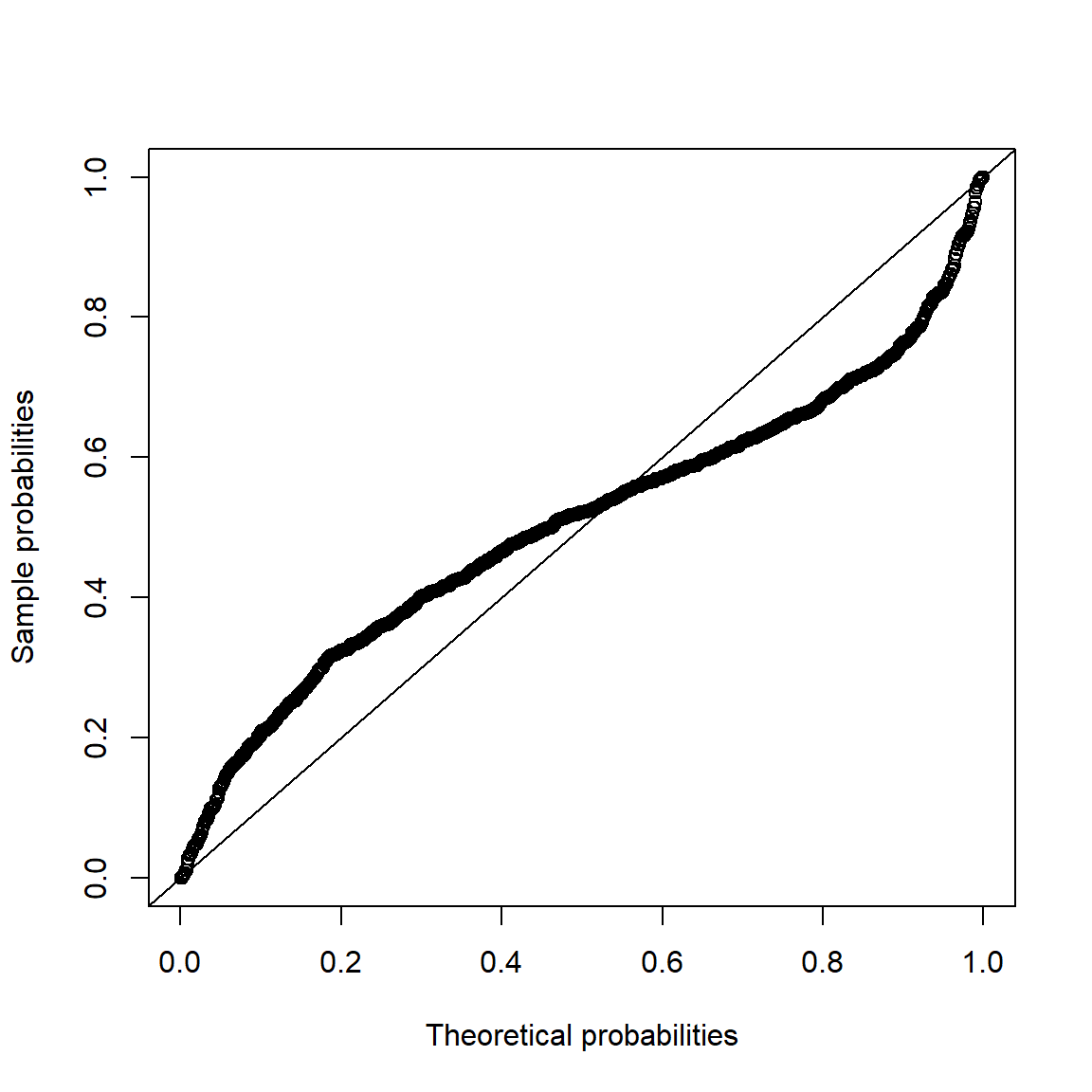
qq_plot(X.t, FUN = function(p) qnorm(p, mean = mu.t, sd = sig.t))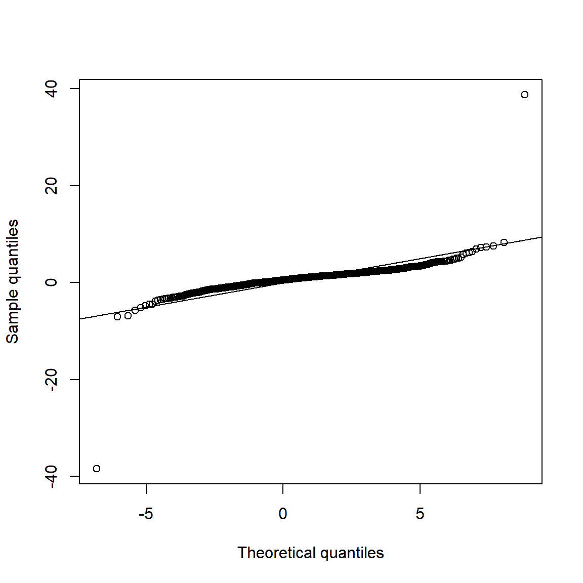
## => S-shape => Data seems to come from heavier-tailed distribution than
##    the normal distribution.
3.4.3 Data application
Prepare risk factor data:
data(DJ_const) # constituents data
margin = c("KO", "MSFT", "INTC", "DIS") # margins considered
DJ.const = DJ_const['1993-01-01/2000-12-31', margin]
X = -returns(DJ.const) # compute -log-returns; daily risk-factor changes
X. = list(daily = X, # daily risk-factor changes
          weekly = apply.weekly(X, FUN = colSums), # weekly risk-factor changes
          monthly = apply.monthly(X, FUN = colSums), # monthly risk-factor changes
          quarterly = apply.quarterly(X, FUN = colSums)) # quarterly risk-factor changes
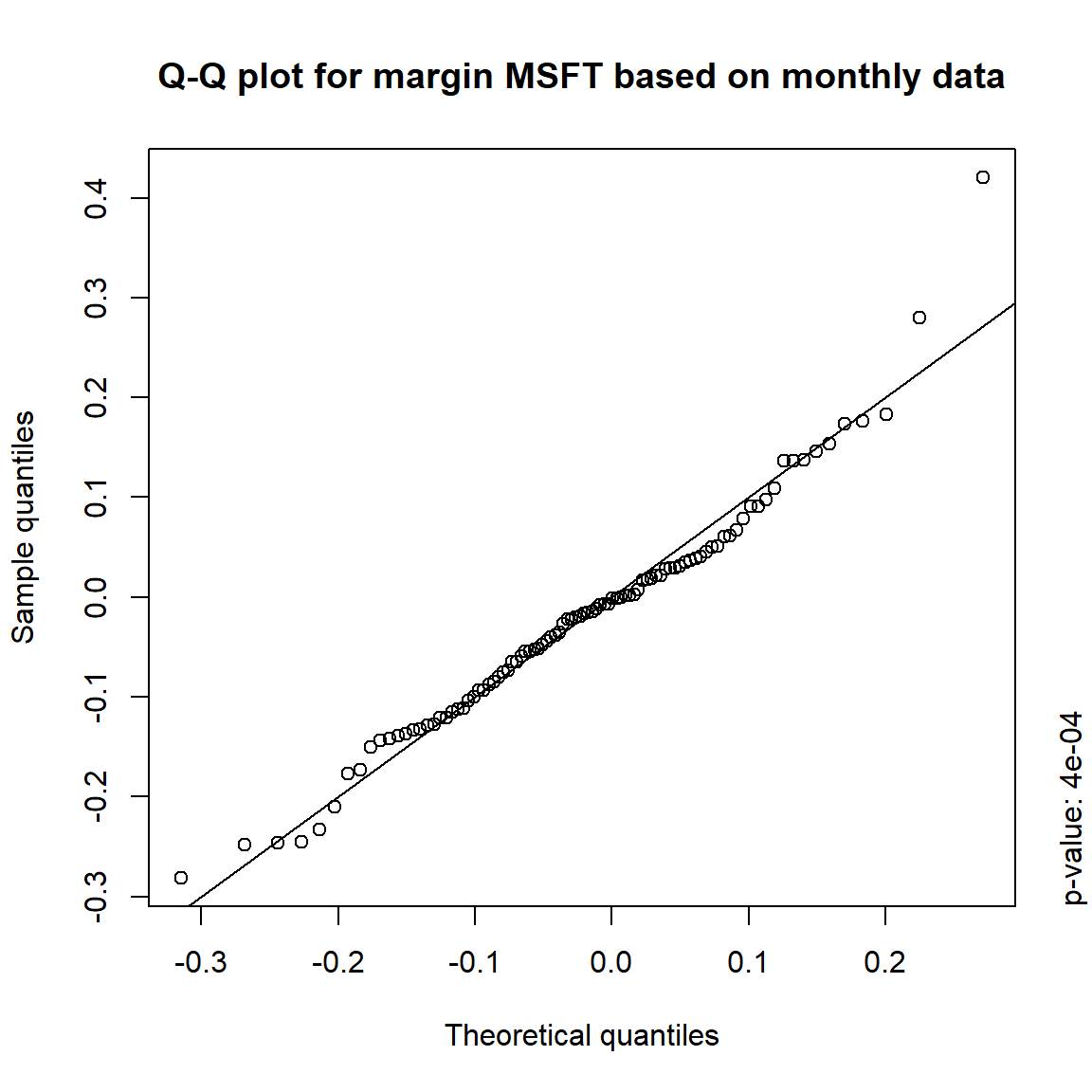
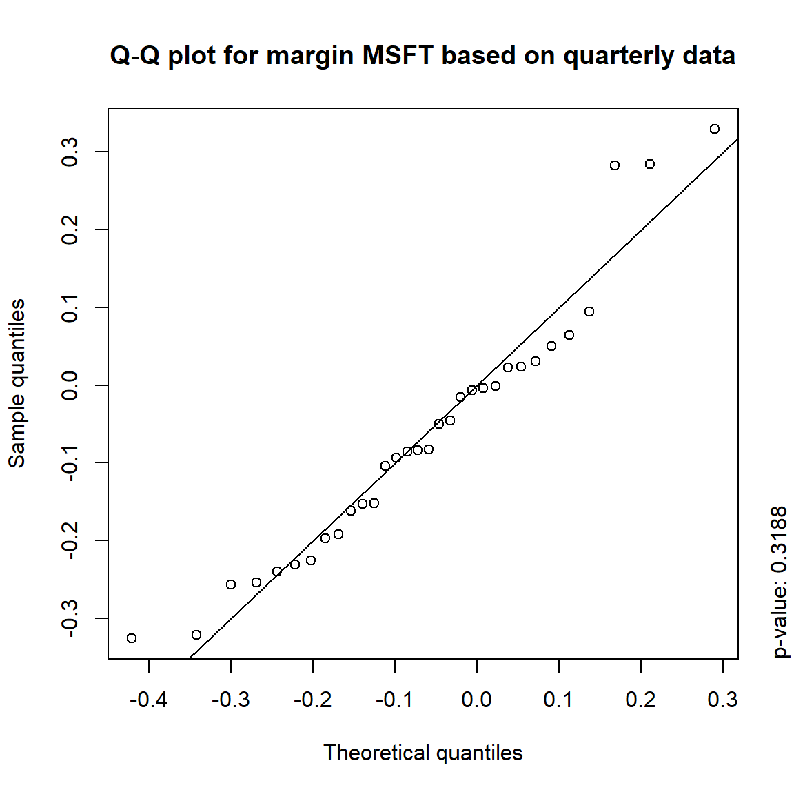
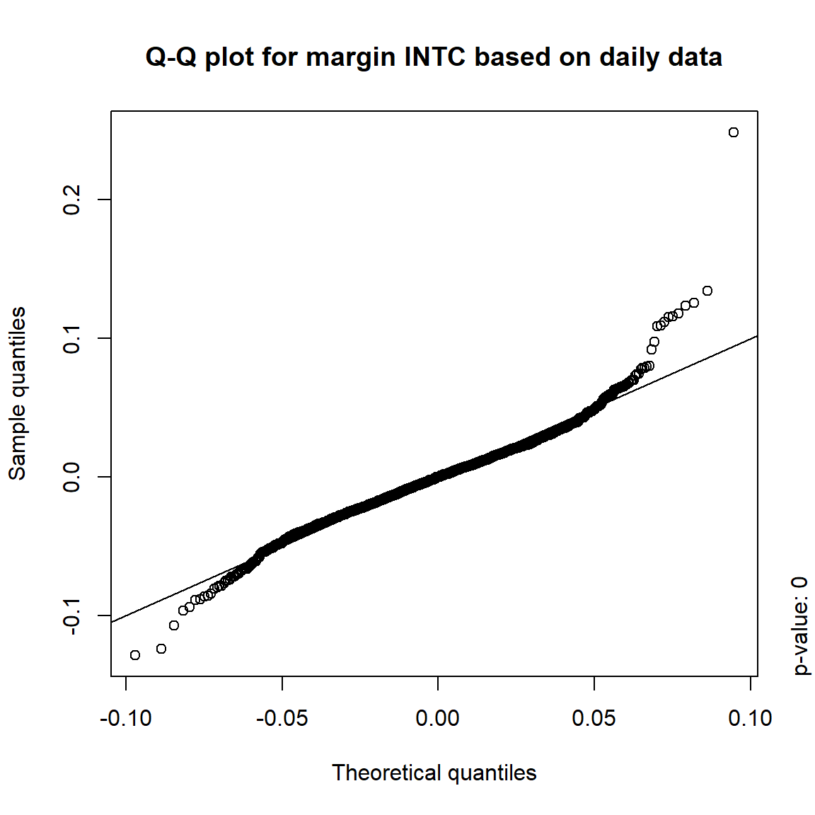
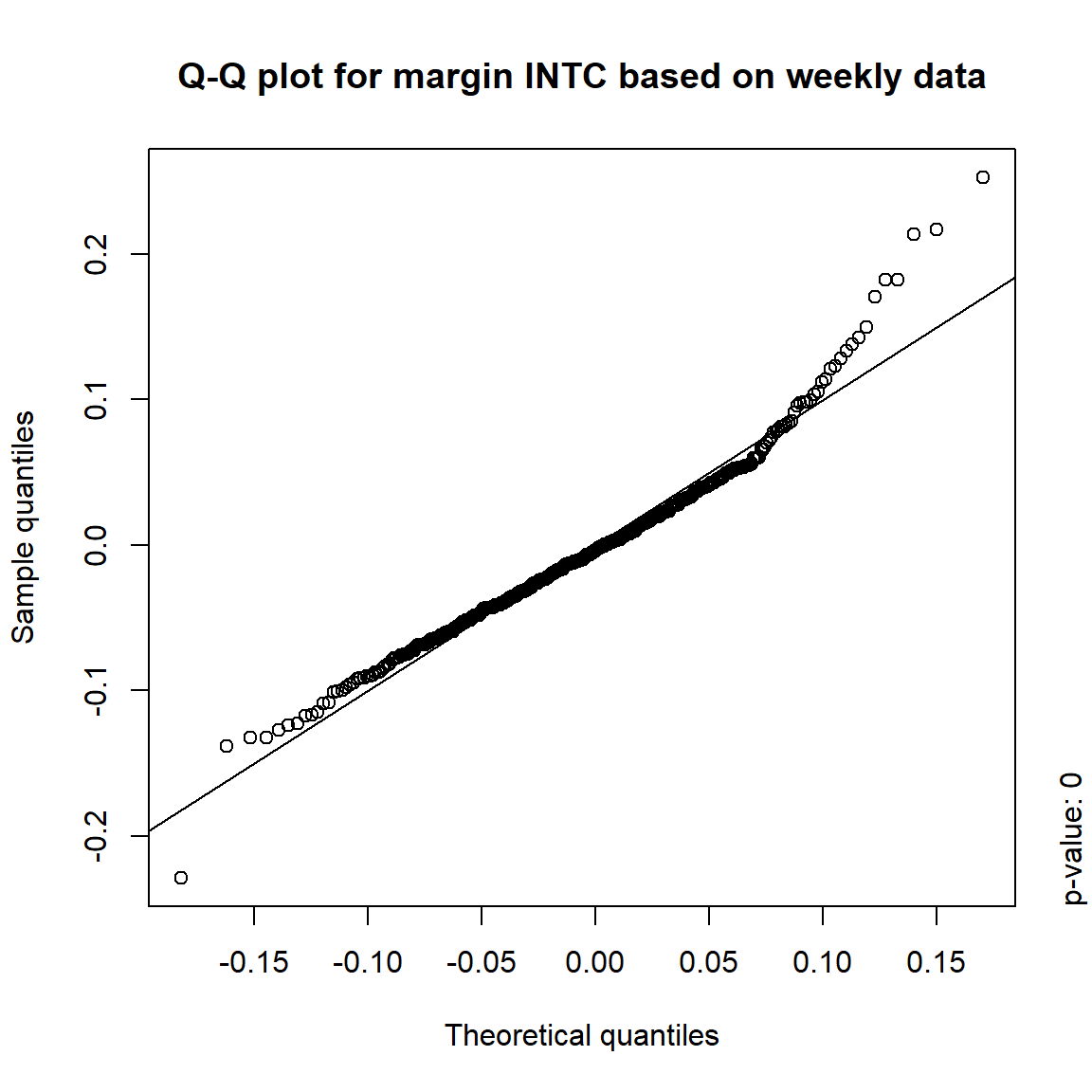
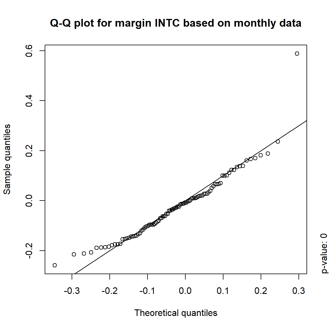
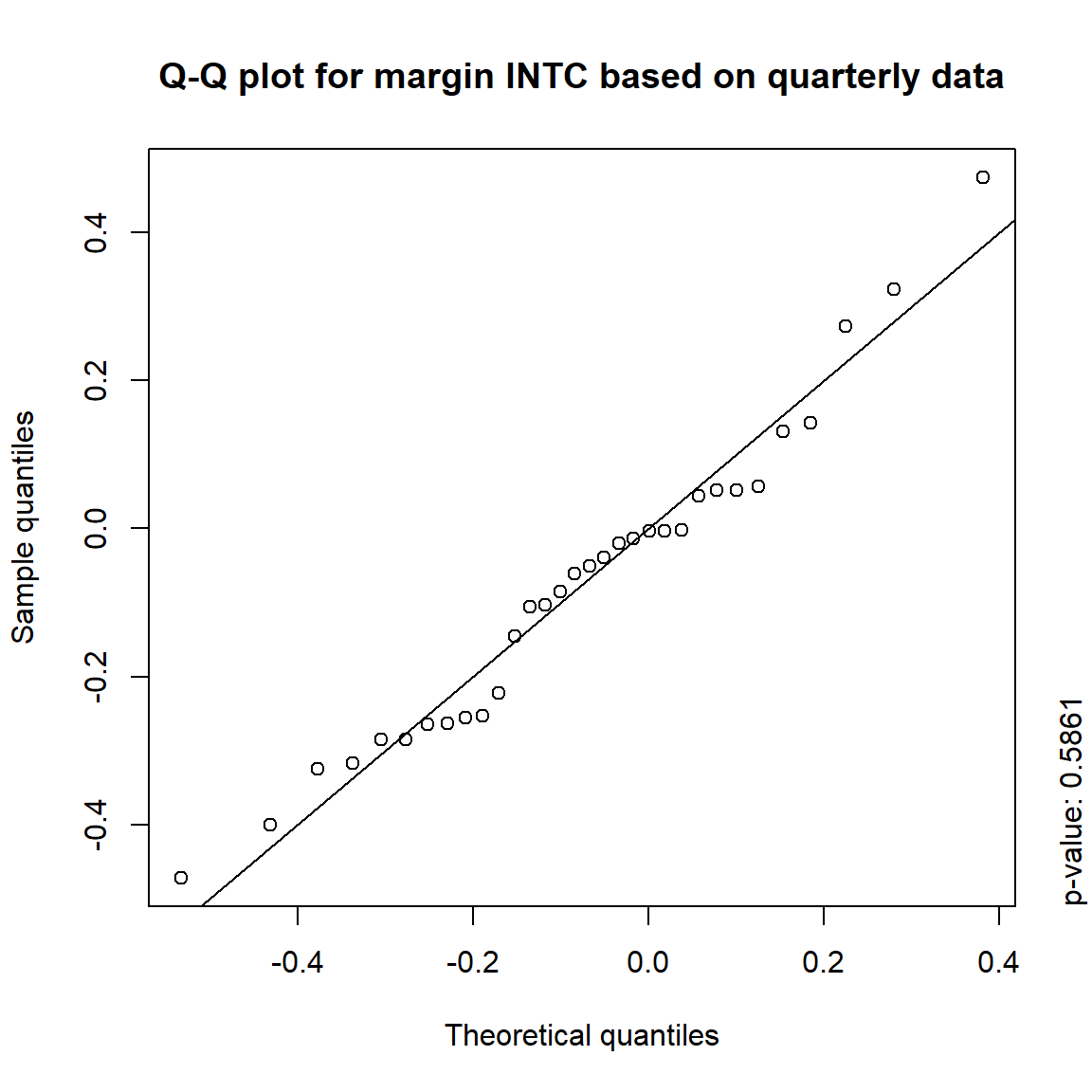
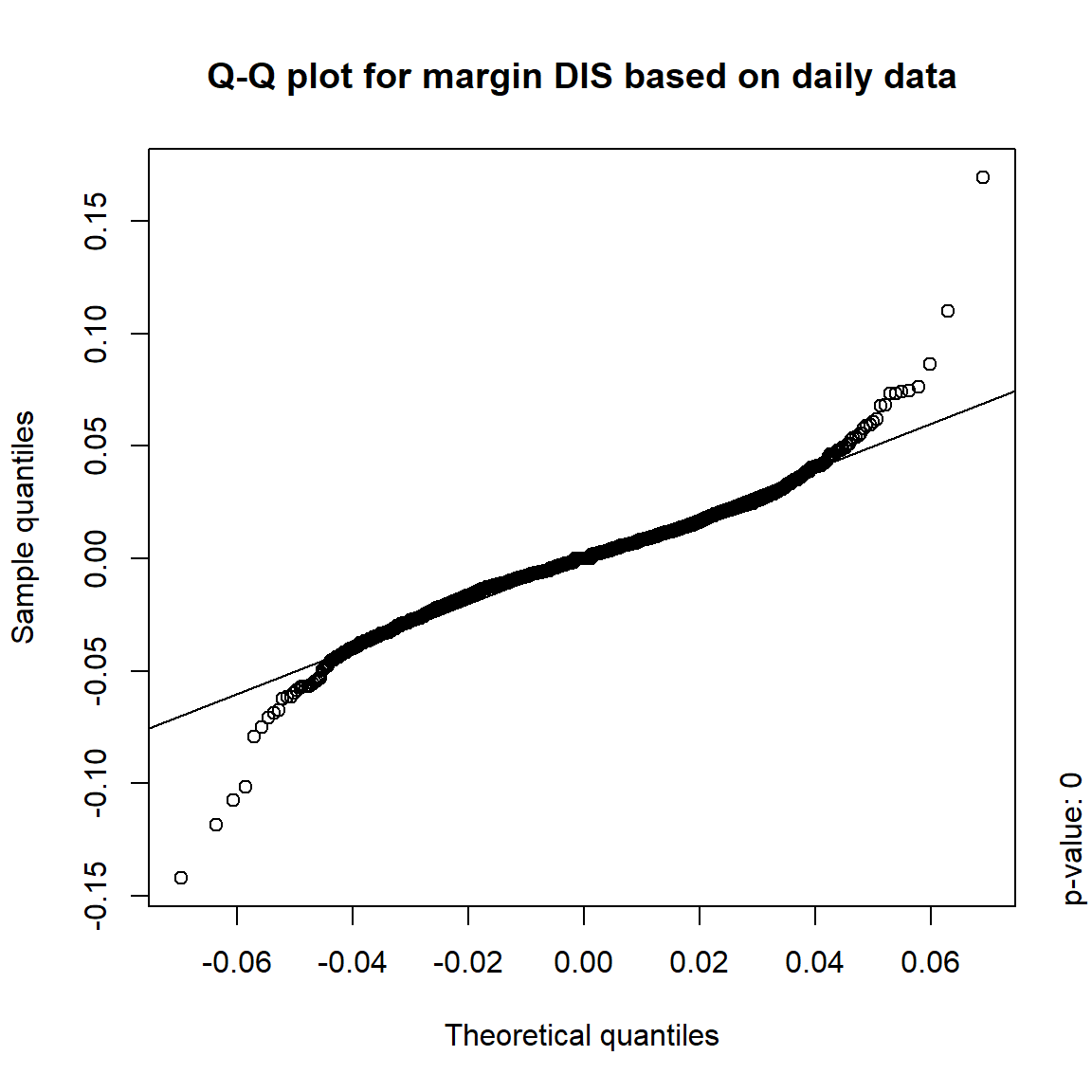
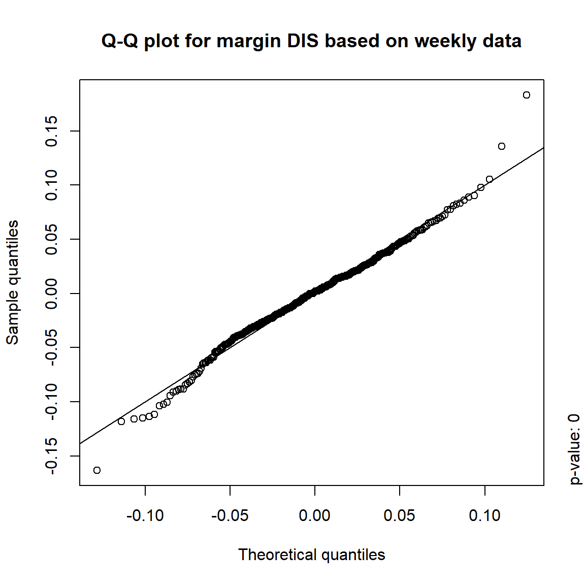
3.4.3.1 Are the risk-factor changes normally distributed?
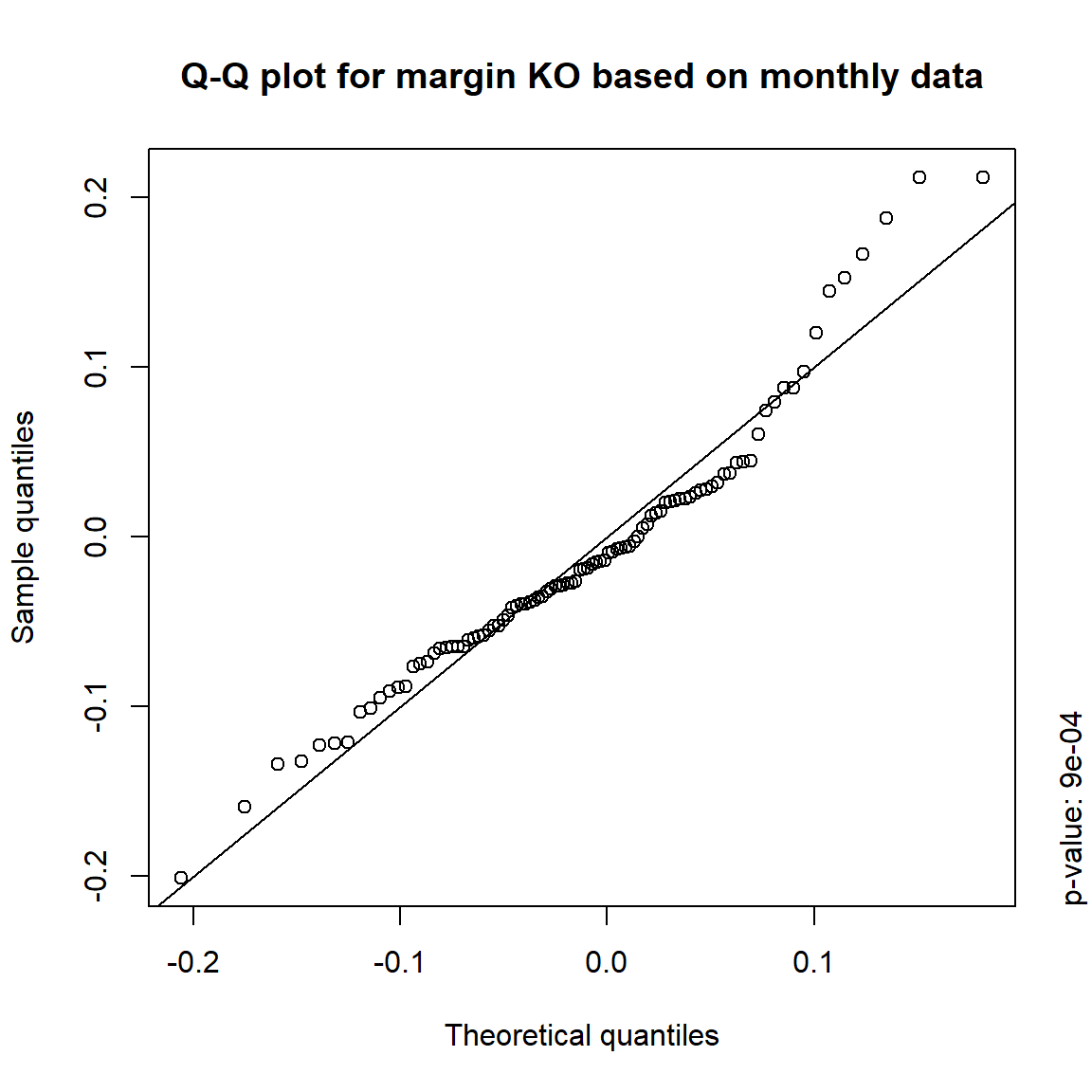
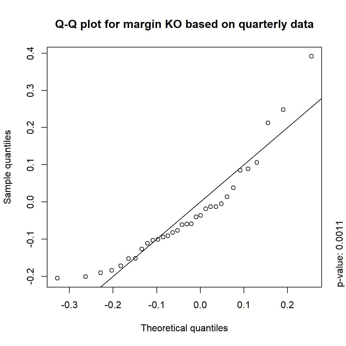
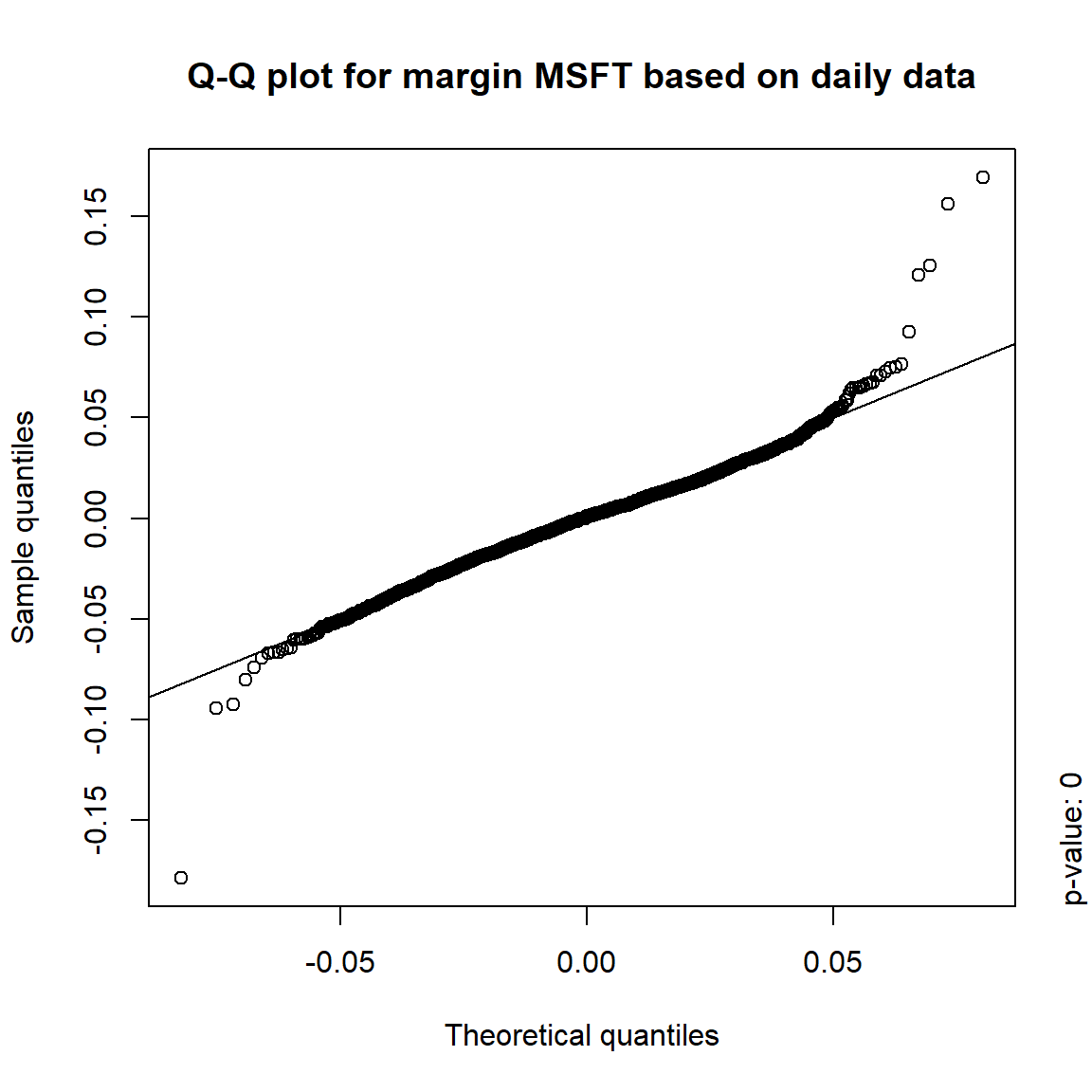
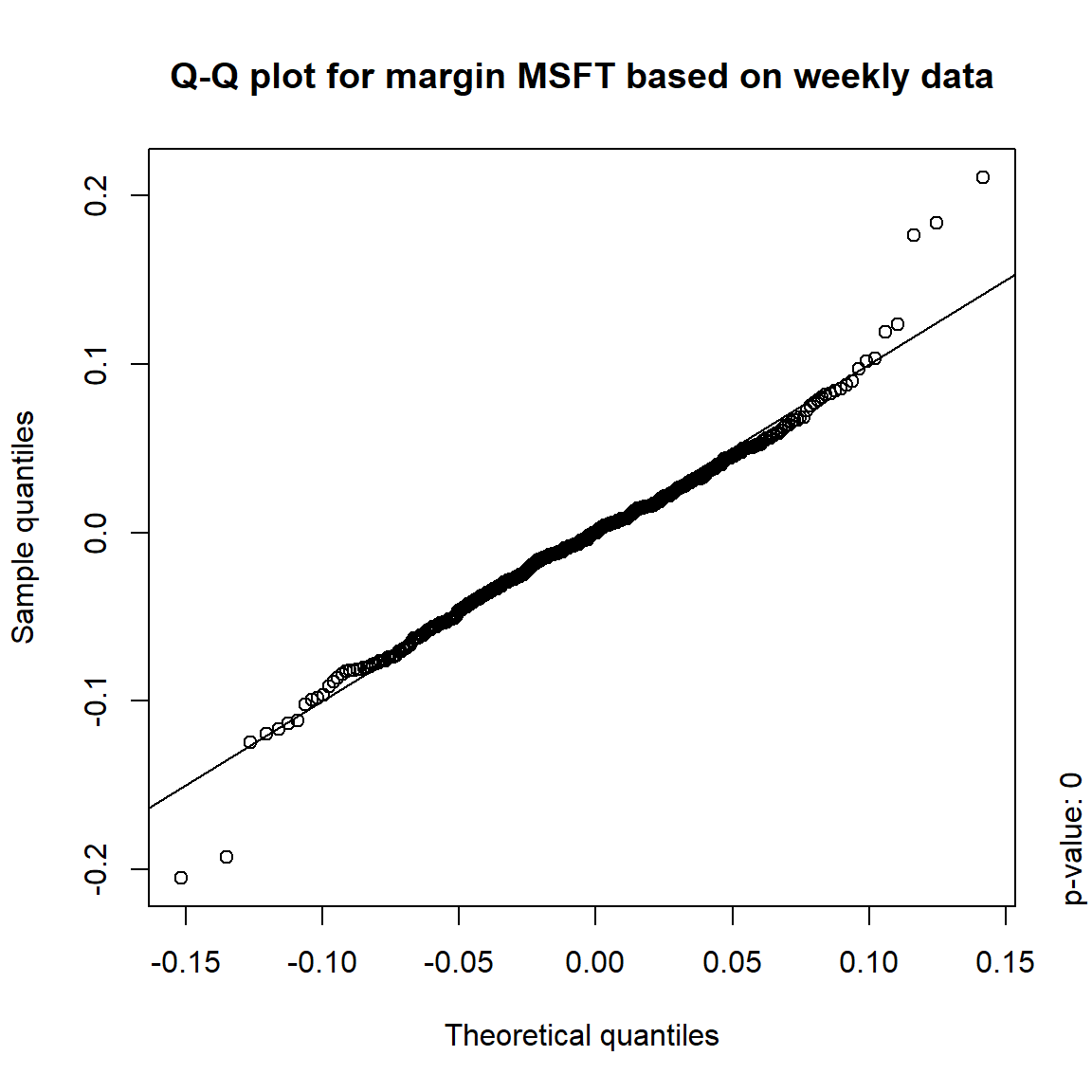
## Formal tests
pvals = sapply(X., function(x) apply(x, 2, function(data) jarque.test(data)$p.value))
pvals < 0.05
## daily weekly monthly quarterly
## KO TRUE TRUE TRUE TRUE
## MSFT TRUE TRUE TRUE FALSE
## INTC TRUE TRUE TRUE FALSE
## DIS TRUE TRUE FALSE FALSE## => Daily and weekly risk-factor changes are not (univariate) normal## Q-Q plots
time = c("daily", "weekly", "monthly", "quarterly")
for(j in seq_len(ncol(X))) { # for all margins, do...
for(k in seq_along(time)) { # for daily, weekly, monthly and quarterly data, do...
qq_plot(X.[[k]][,j], FUN = function(p)
qnorm(p, mean = mean(X.[[k]][,j]), sd = sd(X.[[k]][,j])),
main = paste("Q-Q plot for margin",margin[j],"based on",time[k],"data"))
mtext(paste("p-value:", round(pvals[j,k], 4)), side = 4, line = 1, adj = 0)
}
}

3.4.4 Simulation
Under \(H_0\), p-values are uniformly distributed. Let’s check that for \(\mathcal{N}(0,1)\) data.
set.seed(271)
pvals.H0 = sapply(1:200, function(b) jarque.test(rnorm(n))$p.value)
qq_plot(pvals.H0, FUN = qunif)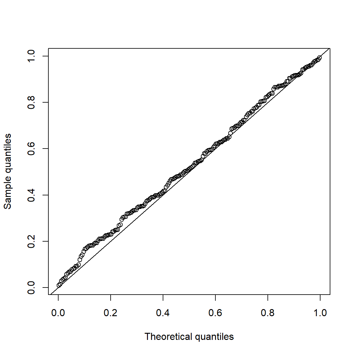
This does not hold under \(H_1\):
set.seed(271)
pvals.H1 = sapply(1:200, function(b) jarque.test(rt(n, df = nu))$p.value)
qq_plot(pvals.H1, FUN = qunif)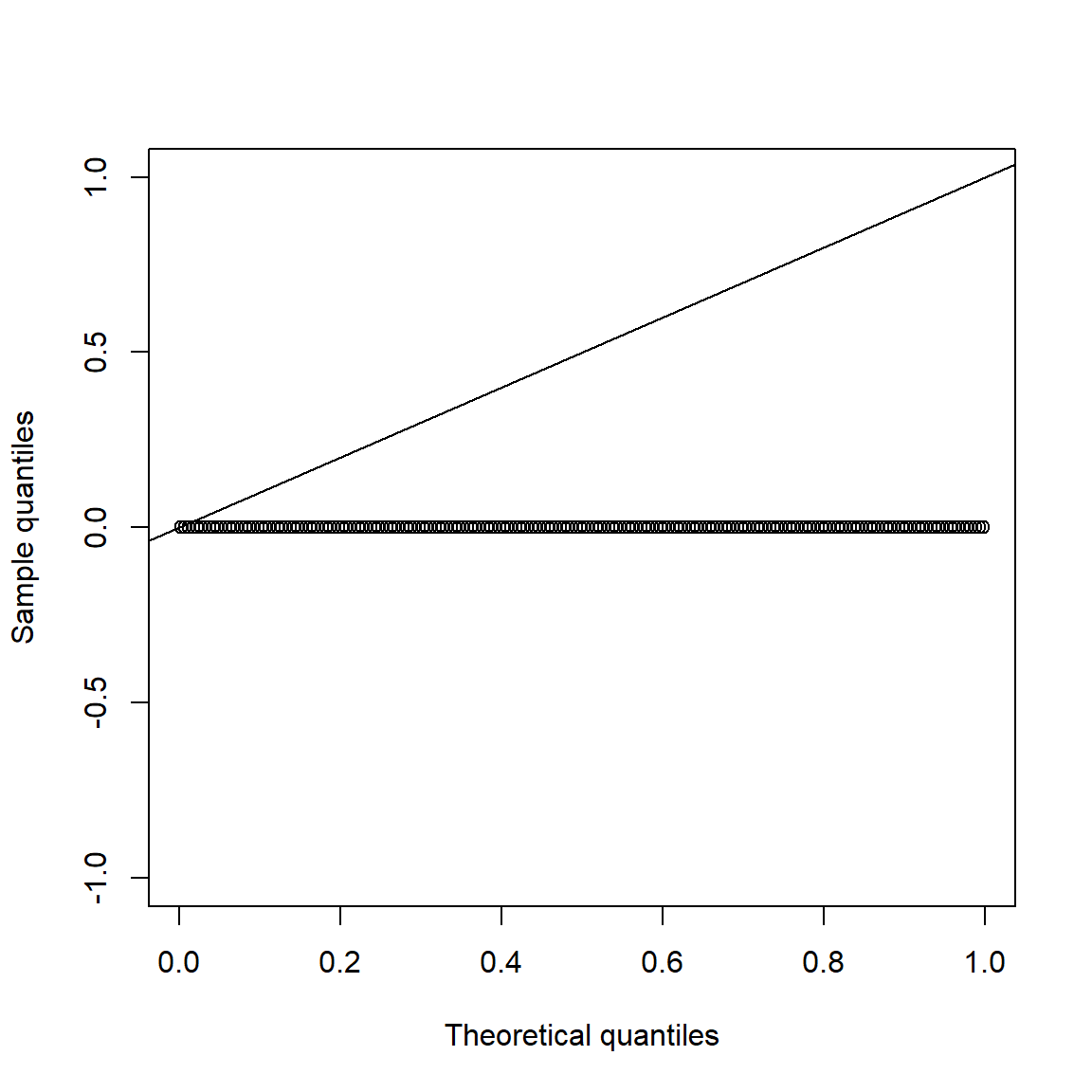
all(pvals.H1 == 0) # all p-values 0## [1] TRUE3.5 Multivariate stylized facts
Illustrates multivariate stylized facts for financial return series.
Multivariate stylized facts:
(M1) Return series show little cross-correlation, except for contemporaneous returns;
(M2) Absolute (or squared) returns show profound cross-correlation;
(M3) Correlations between contemporaneous returns vary over time;
(M4) Extreme returns often coincide with extreme returns in (several) other time series.
library(xts)
library(nvmix) # for rNorm(), rStudent()
library(qrmdata)
library(qrmtools)
3.5.1 Index data
data("FTSE")
data("SMI")
Build log-returns and merge:
FTSE.X = returns(FTSE)
SMI.X = returns(SMI)
X = merge(FTSE = FTSE.X, SMI = SMI.X, all = FALSE)
3.5.2 (M1) and (M2)
(M1) Return series show little cross-correlation, except for contemporaneous returns
(M2) Absolute (or squared) returns show profound cross-correlation
Autocorrelations of returns and absolute returns:
acf(X) # raw values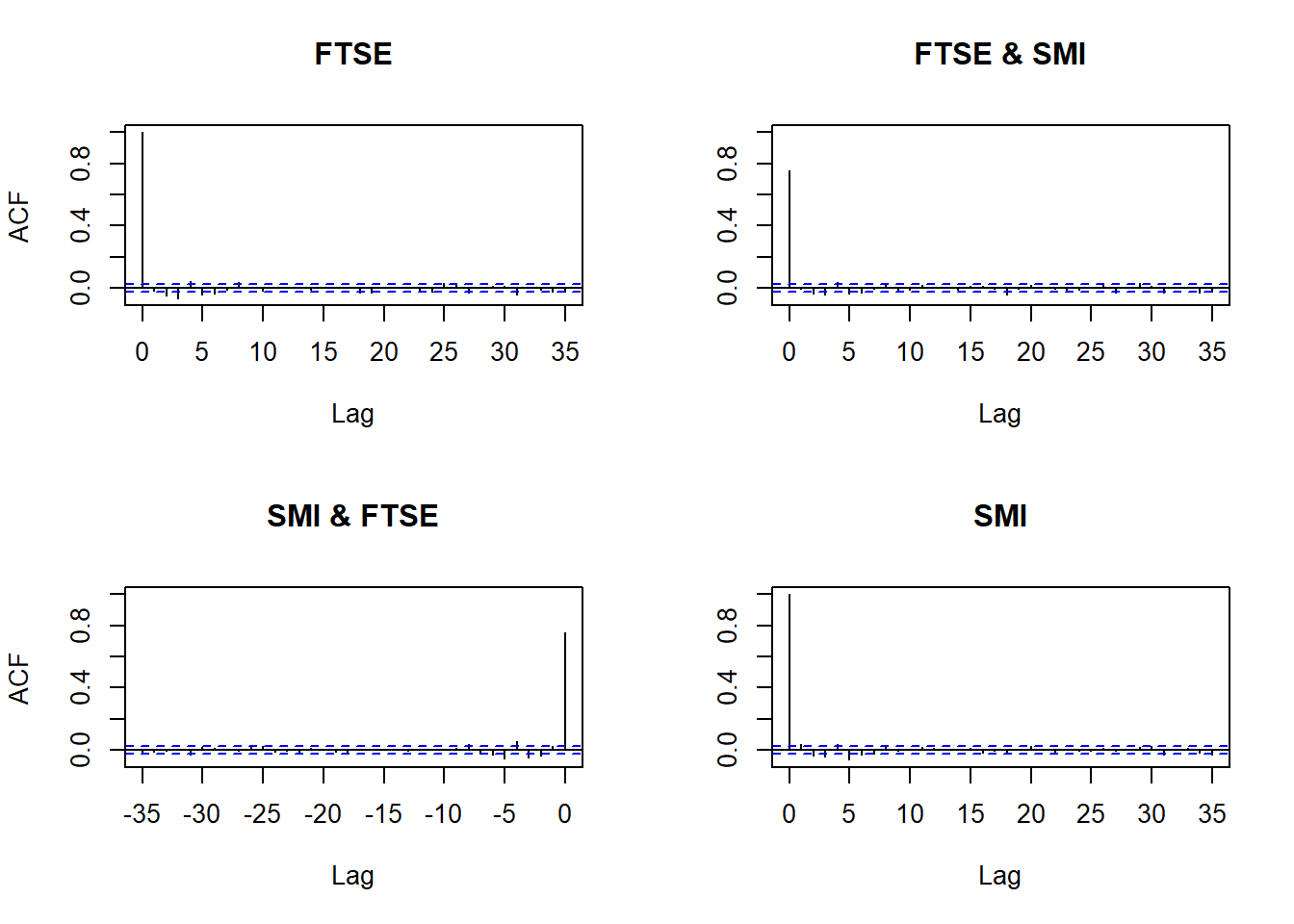
acf(abs(X)) # absolute values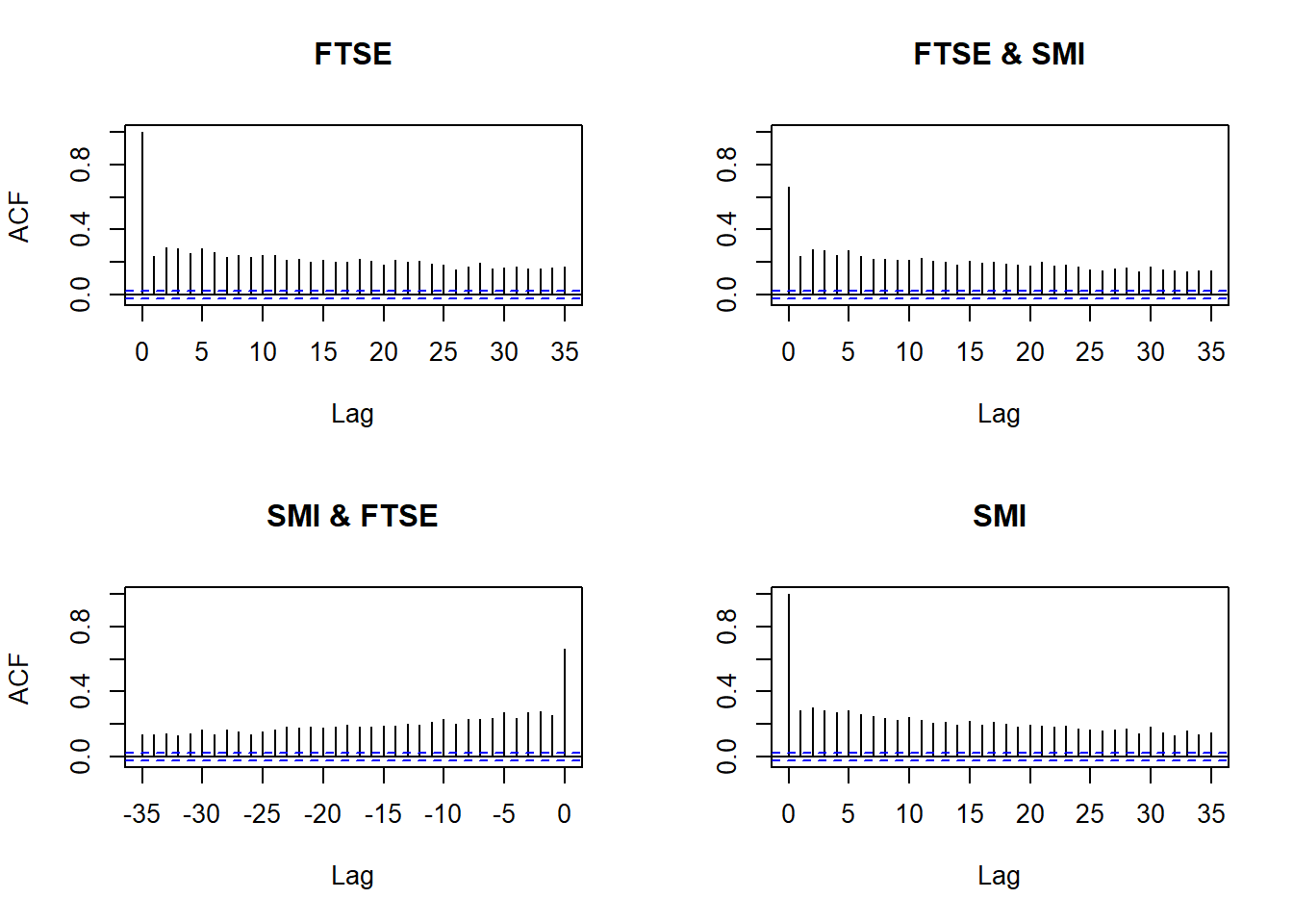
3.5.3 (M3)
- (M3) Correlations between contemporaneous returns vary over time
Plot cross-correlation (and volatilities):
X.cor  = apply.monthly(X, FUN = cor)[,2] # cross-correlations estimated based on monthly non-overlapping windows
X.vols = apply.monthly(X, FUN = function(x) apply(x, 2, sd)) # componentwise volatilities
X.cor.vols = merge(X.cor, X.vols)
names(X.cor.vols) = c("Cross-correlation", "Volatility FTSE", "Volatility SMI")
plot.zoo(X.cor.vols, xlab = "Time", main = "Cross-correlation and volatility estimates")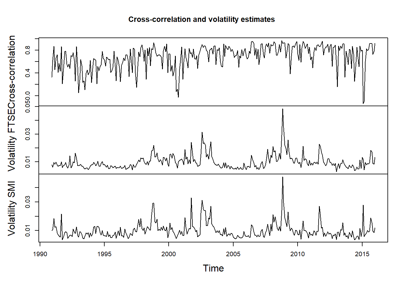
## => Cross-correlation varies over time; below we further investigate the
##    relationship between volatility and cross-correlation
Extract volatilities and compute Fisher-transformed cross-correlations:
The Fisher transformation can be used to test hypotheses about the value of the population correlation coefficient \(\rho\) between variables \(X\) and \(Y\). This is because, when the transformation is applied to the sample correlation coefficient, the sampling distribution of the resulting variable is approximately normal, with a variance that is stable over different values of the underlying true correlation.
Fisher’s transformation of \(\rho\) is defined as \[ z = \frac{1}{2}\log\left(\frac{1+\rho}{1-\rho}\right) \]
The Fisher transform is a wellknown variance-stabilizing transform that is appropriate when correlation is the dependent variable in a regression analysis.
FTSE.sig = as.numeric(X.vols[,"FTSE"])
SMI.sig  = as.numeric(X.vols[,"SMI"])
fisher = function(r) log((1 + r)/(1 - r))/2 # Fisher (z-)transformation
rho = fisher(X.cor) # Fisher transform cross correlations
Plot Fisher-transformed cross-correlation against volatility with regression lines:
Note: If \((X,Y)\) are jointly normal with correlation \(\rho\), fisher’s transformed sample correlation is approximately \(\mathcal{N}\left(\frac{1}{2}\log\left(\frac{1+\rho}{1-\rho}\right), \frac{1}{n-3}\right)\) distributed (\(n\) = sample size).
## FTSE
plot(FTSE.sig, rho, xlab = "Estimated volatility", ylab = "Estimated cross-correlation")
reg = lm(rho ~ FTSE.sig)
summary(reg)
##
## Call:
## lm(formula = rho ~ FTSE.sig)
##
## Residuals:
## Min 1Q Median 3Q Max
## -1.14689484 -0.23532132 0.00702075 0.27898787 0.88317510
##
## Coefficients:
## Estimate Std. Error t value Pr(>|t|)
## (Intercept) 0.58617194 0.04376356 13.39407 < 2.22e-16 ***
## FTSE.sig 36.37913535 3.89888949 9.33064 < 2.22e-16 ***
## ---
## Signif. codes: 0 '***' 0.001 '**' 0.01 '*' 0.05 '.' 0.1 ' ' 1
##
## Residual standard error: 0.3624633 on 300 degrees of freedom
## Multiple R-squared: 0.2249281, Adjusted R-squared: 0.2223445
## F-statistic: 87.06085 on 1 and 300 DF, p-value: < 2.2204e-16abline(reg)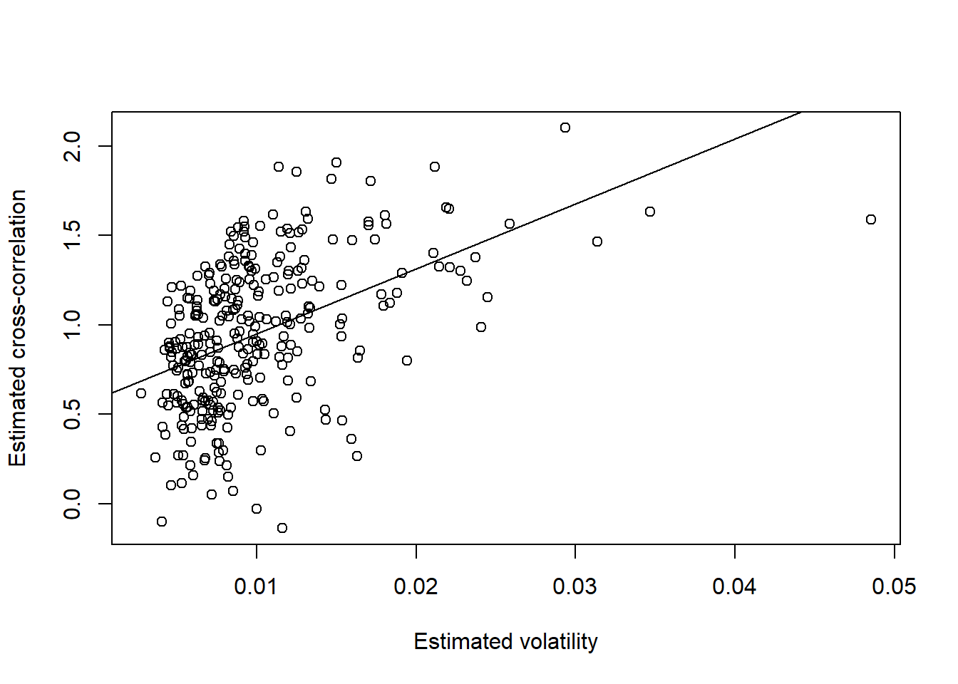
## SMI
plot(SMI.sig, rho, xlab = "Estimated volatility", ylab = "Estimated cross-correlation")
reg = lm(rho ~ SMI.sig)
summary(reg)
##
## Call:
## lm(formula = rho ~ SMI.sig)
##
## Residuals:
## Min 1Q Median 3Q Max
## -1.61462953 -0.25011470 0.00568859 0.25887690 0.91906510
##
## Coefficients:
## Estimate Std. Error t value Pr(>|t|)
## (Intercept) 0.63948644 0.04474835 14.29073 < 2.22e-16 ***
## SMI.sig 30.00745100 3.84716708 7.79988 1.0329e-13 ***
## ---
## Signif. codes: 0 '***' 0.001 '**' 0.01 '*' 0.05 '.' 0.1 ' ' 1
##
## Residual standard error: 0.3754027 on 300 degrees of freedom
## Multiple R-squared: 0.1686024, Adjusted R-squared: 0.165831
## F-statistic: 60.83817 on 1 and 300 DF, p-value: 1.03295e-13abline(reg)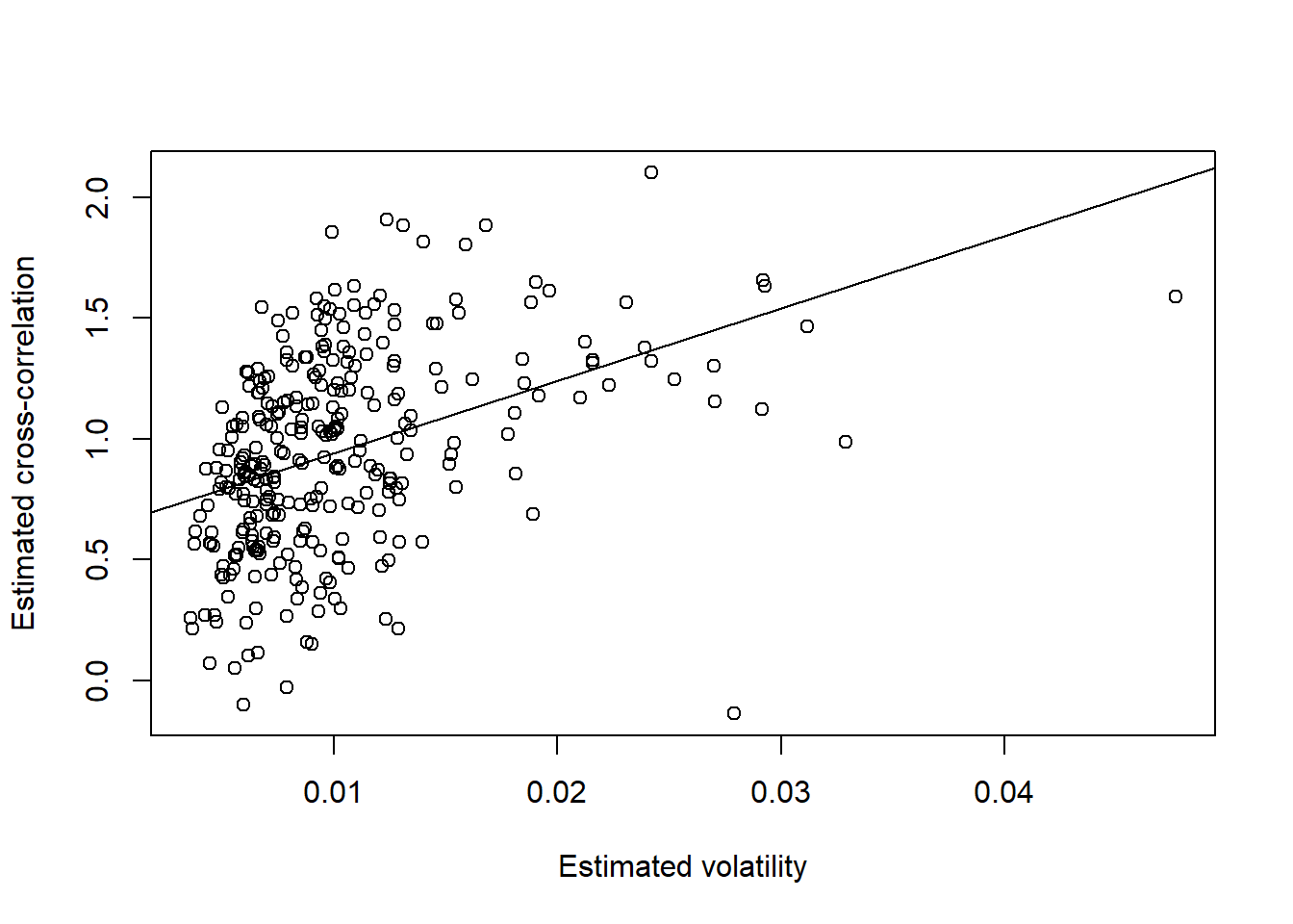
EXERCISE: Now try and compare with these SWN (strict white noise) data:
set.seed(271)
X.t = xts(rStudent(n = nrow(X), df = 3, scale = cor(X)), time(X))
X.N = xts(rNorm(n = nrow(X), scale = cor(X)), time(X))
3.5.4 (M4)
- (M4) Extreme returns often coincide with extreme returns in (several) other time series
plot.zoo(X, xlab = "Time", main = "Log-returns") # seems like extremes occur together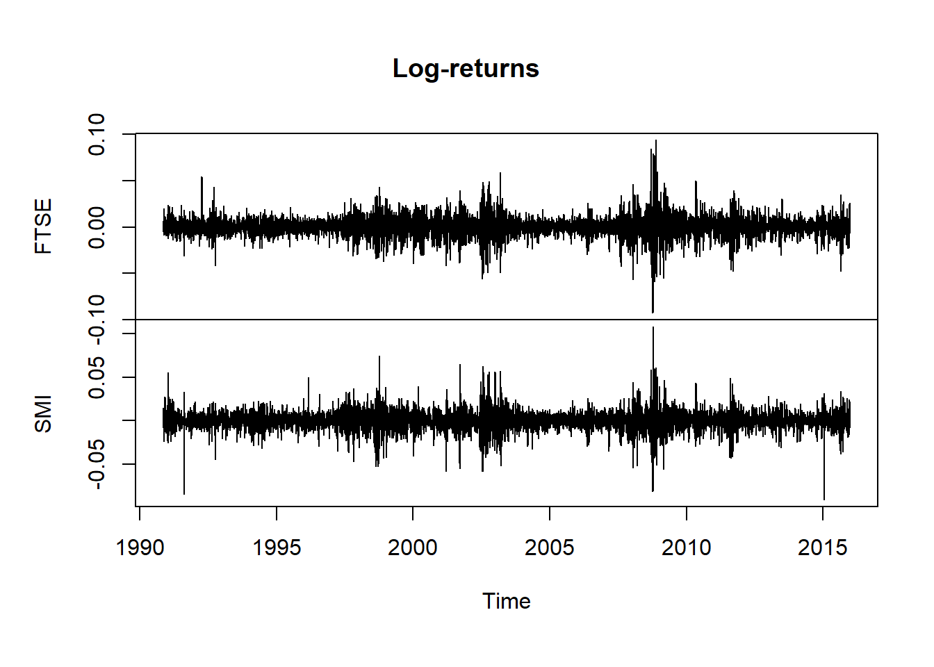
X. = apply(X, 2, rank) / (nrow(X) + 1)
plot(X., main = "Componentwise scaled ranks") # now better visible (bottom-left, top-right corners)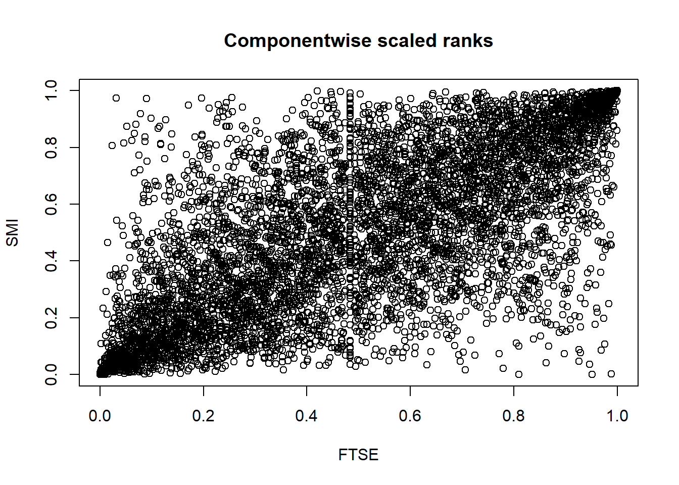
## Note: More on that ("pseudo-observations") in Chapter 7