Chapter 2 Basic Concepts in Risk Management
2.1 Review
2.1.1 Notations
the value of the portfolio at the end of the time period \(V_{t+1}\)
the change in value of the portfolio \(\Delta V_{t+1} = V_{t+1} - V_t\)
loss for short time intervals \(L_{t+1} := -\Delta V_{t+1}\)
typically random from the viewpoint of time \(t\)
has a loss distribution
loss for long time intervals \(V_t - V_{t+1}/(1 + r_{t,1})\)
\(r_{t,1}\) is the simple risk-free interest rate that applies between times \(t\) and \(t+1\)
this measures the loss in units of money at time \(t\)
\(V_t\) has the representation:
\[ V_t = f(t, \boldsymbol{Z}_t), \quad f: \mathbb{R}_+ \times \mathbb{R}^d \rightarrow \mathbb{R} \tag{2.1} \]
\(d\)-dimensional risk factors \(\boldsymbol{Z}_t = (Z_{t,1},...,Z_{t,d})'\)
random vector \(\boldsymbol{Z}_t\) takes some known realized value \(\boldsymbol{z}_t\)
\(V_t\) has realized value \(f(t, \boldsymbol{z}_t)\) at time \(t\)
random vector of risk-factor changes \(\boldsymbol{X}_{t+1} := \boldsymbol{Z}_{t+1} - \boldsymbol{Z}_t\)
at time \(t\) using the mapping Equation (2.1), the portfolio loss is
\[ L_{t+1} = -(f(t+1, \boldsymbol{z}_t + \boldsymbol{X}_{t+1}) - f(t,\boldsymbol{z}_t)) \tag{2.2} \] which shows that the loss distribution is determined by the distribution of the risk-factor change \(\boldsymbol{X}_{t+1}\).
If \(f\) is differentiable, we have first-order approximation of the loss (linearized loss) in Equation (2.2) of the form
\[ L_{t+1}^\Delta := -\left(f_t(t,\boldsymbol{z}_t) + \sum_{i=1}^d f_{z_i}(t, \boldsymbol{z}_t) X_{t+1,i}\right) \tag{2.3} \] where the subscripts on \(f\) denote partial derivatives.
Example 2.1 (stock portfolio) Consider a fixed portfolio of \(d\) stocks and denote by \(\lambda_i\) the number of shares of stock \(i\) in the portfolio at time \(t\). The price process of stock \(i\) is denoted by \((S_{t,i})_{t\in \mathbb{N}}\).
Following standard practice in finance and risk management we use logarithmic prices as risk factors, i.e. we take \(Z_{t,i} := \ln{S_{t,i}}, \ 1 \leq i \leq d\), and we get \(V_t = \sum_{i=1}^d \lambda_i e^{Z_{t,i}}\). The risk-factor changes \(X_{t+1,i} = \ln{S_{t+1,i}} −\ln{S_{t,i}}\) then correspond to the log-returns of the stocks in the portfolio.The portfolio loss from time \(t\) to \(t+1\) is given by \[ L_{t+1} = -(V_{t+1}-V_t) = - \sum_{i=1}^d \lambda_i S_{t,i} (e^{X_{t+1,i}}-1) \] and the linearized loss \[ L_{t+1}^\Delta = - \sum_{i=1}^d \lambda_i S_{t,i} X_{t+1,i} = - V_t \sum_{i=1}^d w_{t,i} X_{t+1,i} \tag{2.4} \] where the weight \(w_{t,i} := (\lambda_i S_{t,i})/V_t\) gives the proportion of the portfolio value invested in stock \(i\) at time \(t\).
Suppose that the random vector \(\boldsymbol{X}_{t+1}\) has a distribution with mean vector \(\boldsymbol{\mu}\) and covariance matrix \(\boldsymbol{\Sigma}\). We have \[ E(L_{t+1}^\Delta) = - V_t \boldsymbol{w}' \boldsymbol{\mu} \quad \text{and} \quad Var(L_{t+1}^\Delta) = V_t^2 \boldsymbol{w}' \boldsymbol{\Sigma} \boldsymbol{w} \tag{2.5} \]
\(\blacksquare\)
2.1.2 Value-at-Risk (VaR)
Consider a portfolio of risky assets and a fixed time horizon \(\Delta t\), and denote by \(F_L(l) = P(L \leq l)\) the distribution function of the corresponding loss distribution. We want to define a statistic based on \(F_L\) that measures the severity of the risk of holding our portfolio over the time period \(\Delta t\).
An obvious candidate is the maximum possible loss, given by \(\inf\{l \in \mathbb{R}: F_L(l) = 1\}\). However, for most distributions of interest, the maximum loss is infinity. Moreover, by using the maximum loss, any probability information in \(F_L\) is neglected.
The idea in the definition of VaR is to replace “maximum loss” by “maximum loss that is not exceeded with a given high probability”.
Definition 2.1 (value-at-risk) Given some confidence level \(\alpha \in (0, 1)\), the VaR of a portfolio with loss \(L\) at the confidence level \(\alpha\) is given by the smallest number \(l\) such that the probability that the loss \(L\) exceeds \(l\) is no larger than \(1 − \alpha\). Formally, \[ \text{VaR}_\alpha = \text{VaR}_\alpha (L) = \inf \{l \in \mathbb{R} : P(L > l) \leq 1 - \alpha\} = \inf \{l \in \mathbb{R} : F_L(l) \geq \alpha\}. \tag{2.6} \]
MFE (2015, Definition 2.8)\(\blacksquare\)
In probabilistic terms, VaR is therefore simply a quantile of the loss distribution. The interpretation is if the 95% VaR value is 2.2, then there is a 5% chance that we lose at least this amount.
Definition 2.2 (the generalized inverse and the quantile function)
Given some increasing function \(T : \mathbb{R} \rightarrow \mathbb{R}\), the generalized inverse of \(T\) is defined by \(T^{\leftarrow}(y) := \inf\{x \in \mathbb{R}: T (x) \geq y\}\), where we use the convention that the infimum of an empty set is .
Given some distribution function \(F\), the generalized inverse \(F^{\leftarrow}\) is called the quantile function of \(F\). For \(\alpha \in (0, 1)\) the \(\alpha\)-quantile of \(F\) is given by \[ q_{\alpha}(F) := F^{\leftarrow}(\alpha) = \inf \{x \in \mathbb{R}: F(x) \geq \alpha \}. \]
\(\blacksquare\)
If \(F\) is continuous and strictly increasing, we simply have \(q_{\alpha}(F) = F^{-1}(\alpha)\), where \(F^{-1}\) is the ordinary inverse of \(F\).
Lemma 2.1 A point \(x_0 \in \mathbb{R}\) is the \(\alpha\)-quantile of some distribution function \(F\) if and only if the following two conditions are satisfied: \(F(x_0) \geq \alpha\); and \(F(x) < \alpha\) for all \(x < x_0\).
MFE (2015, Lemma 2.10)\(\blacksquare\)
The lemma follows immediately from the definition of the generalized inverse and the right-continuity of \(F\).
Example 2.2 (VaR for normal and \(t\) loss distribution)
Suppose that the loss distribution \(F_L\) is normal with mean \(\mu\) and variance \(\sigma^2\). Fix \(\alpha \in (0, 1)\). Then \[ \text{VaR}_{\alpha} = \mu + \sigma \Phi^{-1} (\alpha) \tag{2.7} \] where \(\Phi\) denotes the standard normal df and \(\Phi^{−1}(\alpha)\) is the \(\alpha\)-quantile of \(\Phi\). The proof is easy: since \(F_L\) is strictly increasing, by Lemma 2.1 we only have to show that \(F_L(\text{VaR}_{\alpha}) = \alpha\). Now, \[ P(L \leq \text{VaR}_{\alpha}) = P\left( \frac{L-\mu}{\sigma} \leq \Phi^{-1}(\alpha) \right) = \Phi (\Phi^{-1} (\alpha)) = \alpha. \] This result is routinely used in the variance–covariance approach (also known as the delta-normal approach) to computing risk measures.
Similarly, suppose that our loss \(L\) is such that \((L − \mu)/\sigma\) has a standard \(t\) distribution with \(\nu\) degrees of freedom; we denote this loss distribution by \(L \sim t(\nu,\mu,\sigma^2)\) and note that the moments are given by \(E(L) = \mu\) and \(Var(L) = \nu\sigma^2/(\nu−2)\) when \(\nu >2\), so \(\sigma\) is not the standard deviation of the distribution. We get \[ \text{VaR}_{\alpha} = \mu + \sigma t_{\nu}^{-1} (\alpha) \tag{2.8} \] where \(t_\nu\) denotes the distribution function of a standard \(t\) distribution.
\(\blacksquare\)
2.1.3 Expected Shortfall (ES)
ES is closely related to VaR and there is an ongoing debate in the risk-management community on the strengths and weaknesses of both risk measures.
Definition 2.3 (expected shortfall) For a loss \(L\) with \(E(|L|) < \infty\) and distribution function \(F_L\), the ES at confidence level \(\alpha \in (0, 1)\) is defined as \[ \text{ES}_\alpha = \frac{1}{1-\alpha} \int_{\alpha}^1 q_u(F_L) \,du \tag{2.9} \] where \(q_u(F_L) = F_L^{\leftarrow}(u)\) is the quantile function of \(F_L\).
MFE (2015, Definition 2.12)\(\blacksquare\)
By definition, ES is related to VaR by \[ \text{ES}_\alpha = \frac{1}{1-\alpha} \int_{\alpha}^1 \text{VaR}_u(L) \,du \] Instead of fixing a particular confidence level \(\alpha\), we average VaR over all levels \(u \geq \alpha\) and thus “look further into the tail” of the loss distribution. Obviously, \(\text{ES}_\alpha\) depends only on the distribution of \(L\), and \(\text{ES}_\alpha \geq \text{VaR}_\alpha\).
Lemma 2.2 For an integrable loss \(L\) with continuous distribution function \(F_L\) and for any \(\alpha \in (0, 1)\) we have \[ \text{ES}_\alpha = \frac{E(L; L \geq q_\alpha (L))}{1-\alpha} = E(L|L\geq \text{VaR}_\alpha) \] where we have used the notation \(E(X; A) := E(X I_A)\) for a generic integrable random variable \(X\) and a generic set \(A \in \mathcal{F}\).
MFE (2015, Lemma 2.13)\(\blacksquare\)
Example 2.3 (expected shortfall for Gaussian loss distribution) Suppose that the loss distribution \(F_L\) is normal with mean \(\mu\) and variance \(\sigma^2\). Fix \(\alpha \in (0, 1)\). Then \[ \text{ES}_\alpha = \mu + \sigma \frac{\phi(\Phi^{-1}(\alpha))}{1-\alpha} \tag{2.10} \] where \(\phi\) is the density of the standard normal distribution. The proof is elementary. First note that \[ \text{ES}_\alpha = \mu + \sigma E\left( \frac{L-\mu}{\sigma} \middle| \frac{L-\mu}{\sigma} \geq q_\alpha \left( \frac{L-\mu}{\sigma} \right) \right); \] hence, it suffices to compute the ES for the standard normal random variable \(\tilde{L} := (L - \mu)/\sigma\). Here we get \[ \text{ES}_\alpha (\tilde{L}) = \frac{1}{1-\alpha} \int_{\Phi^{-1}(\alpha)}^\infty l \phi(l) \,dl = \frac{1}{1-\alpha}[-\phi(l)]_{\Phi^{-1}(\alpha)}^{\infty} = \frac{\phi(\Phi^{-1}(\alpha))}{1-\alpha} \]
MFE (2015, Example 2.14)\(\blacksquare\)
Example 2.4 (expected shortfall for the Student \(t\) loss distribution) Suppose the loss \(L\) is such that \(\tilde{L} = (L−\mu)/\sigma\) has a standard \(t\) distribution with \(\nu\) degrees of freedom, as in Example 2.2. Suppose further that \(\nu >1\). By the reasoning of Example 2.3, we have \(\text{ES}_\alpha = \mu + \sigma \text{ES}_\alpha (\tilde{L})\). The ES of the standard \(t\) distribution is calculated by direct integration to be \[ \text{ES}_\alpha (\tilde{L}) = \frac{g_\nu (t_\nu^{-1} (\alpha))}{1-\alpha} \frac{\nu + (t_\nu^{-1} (\alpha))^2}{\nu - 1} \tag{2.11} \] where \(t_\nu\) denotes the distribution function and \(g_\nu\) the density of standard \(t\).
MFE (2015, Example 2.15)\(\blacksquare\)
Since \(\text{ES}_\alpha\) can be thought of as an average over all losses that are greater than or equal to \(\text{VaR}_\alpha\), it is sensitive to the severity of losses exceeding \(\text{VaR}_\alpha\).
2.2 VaR and ES tail comparison for normal and \(t\) loss distriubion
However, VaR (or ES) does not always give larger values for the \(t\) than the normal distribution; see MFE (2015, Example 2.16).
2.2.1 Setup
Example 2.5 (VaR and ES for stock returns) We consider daily losses on a position in a particular stock; the current value of the position equals \(V_t = 10000\).
Recall from Example 2.1 that the loss for this portfolio is given by \(L_{t+1}^\Delta = −V_t X_{t+1}\), where \(X_{t+1}\) represents daily log-returns of the stock.
We assume that \(X_{t+1}\) has mean \(0\) and standard deviation \(\sigma = 0.2/\sqrt{250}\), i.e. we assume that the stock has an annualized volatility of 20%. We compare two different models for the distribution: namely,
a normal distribution, and
a \(t\) distribution with \(\nu = 4\) degrees of freedom scaled to have standard deviation \(\sigma\).
The \(t\) distribution is a symmetric distribution with heavy tails, so that large absolute values are much more probable than in the normal model.
In case (i), ES for the normal model has been computed using Equation (2.10); in case (ii), the ES for the t model has been computed using Equation (2.11).
\(\blacksquare\)
library(qrmtools)## Registered S3 method overwritten by 'quantmod':
## method from
## as.zoo.data.frame zoo2.2.2 Auxiliary computations
Computing VaR and ES
for a normal and \(t\) distribution for \(X_{t+1}\) (or the linearized loss derived from \(X_{t+1}\)).
Note that the variance for the \(t\) distribution is \(\sigma^2 = \nu\cdot \text{scale}^2/(\nu - 2)\). Thus, the scale parameter for the \(t\) distribution is \(\sigma \sqrt{(\nu-2)/\nu}\).
V = 10000 # value of the portfolio today
sig = 0.2/sqrt(250) # daily volatility (annualized volatility of 20%)
nu = 4 # degrees of freedom for the t distribution
alpha = seq(0.001, 0.999, 0.001) # confidence levels; concentrated near 1
VaR.n = VaR_t(alpha, scale = V*sig, df = Inf) # VaR_alpha under normal
VaR.t = VaR_t(alpha, scale = V*sig*sqrt((nu-2)/nu), df = nu) # VaR_alpha under t
ES.n  = ES_t (alpha, scale = V*sig, df = Inf) # ES_alpha under normal
ES.t  = ES_t (alpha, scale = V*sig*sqrt((nu-2)/nu), df = nu) # ES_alpha under t
2.2.3 Plot
plot(1-alpha, ES.t, col = "maroon3", type = "l", log = "x",
     ylim = range(VaR.n, VaR.t, ES.n, ES.t), xlab = expression(1-alpha), ylab = "")
lines(1-alpha, ES.n,  col = "royalblue3")
lines(1-alpha, VaR.t, col = "darkorange2", lty = 2)
lines(1-alpha, VaR.n, col = "black", lty = 2)
legend("topright", bty = "n", lty = c(1,1,2,2), col = c("maroon3", "royalblue3",
                                                        "darkorange2", "black"),
       legend = c(substitute(ES[alpha]~~"for "*italic(t[nu.])*" model", list(nu. = nu)),
                  expression(ES[alpha]~~"for normal model"),
                  substitute(VaR[alpha]~~"for "*italic(t[nu.])*" model", list(nu. = nu)),
                  expression(VaR[alpha]~~"for normal model")))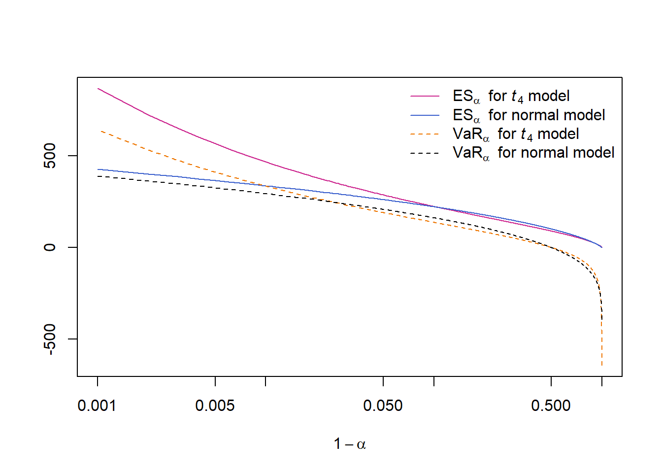
2.2.4 Results
This shows that \(\text{VaR}_\alpha\) (or \(\text{ES}_\alpha\)) is not always ‘riskier’ for the \(t\) distribution than it is for the normal distribution (only for sufficiently large \(\alpha\)).
res.table = round(rbind(alpha, VaR.n, VaR.t, ES.n, ES.t)[,c(900,950,975,990,995)],3)
rownames(res.table) = c("$\\alpha$",
                        "$\\text{VaR}_{\\alpha}$ (normal model)",
                        "$\\text{VaR}_{\\alpha}$ ($t$ model)",
                        "$\\text{ES}_{\\alpha}$ (normal model)",
                        "$\\text{ES}_{\\alpha}$ ($t$ model)")
knitr::kable(
  res.table, booktabs = TRUE,
  caption = "$\\text{VaR}_{\\alpha}$ and $\\text{ES}_{\\alpha}$ in the normal
  and $t$ models for different values of $\\alpha$."
)
## Warning in kable_pipe(x = structure(c("$\\alpha$", "$\\text{VaR}_{\\alpha}$
## (normal model)", : The table should have a header (column names)| \(\alpha\) | 0.900 | 0.950 | 0.975 | 0.990 | 0.995 |
| \(\text{VaR}_{\alpha}\) (normal model) | 162.105 | 208.059 | 247.918 | 294.262 | 325.819 |
| \(\text{VaR}_{\alpha}\) (\(t\) model) | 137.134 | 190.678 | 248.333 | 335.137 | 411.803 |
| \(\text{ES}_{\alpha}\) (normal model) | 221.990 | 260.915 | 295.711 | 337.126 | 365.806 |
| \(\text{ES}_{\alpha}\) (\(t\) model) | 223.548 | 286.473 | 357.195 | 466.943 | 565.710 |
MFE (2015, Table 2.3)
Most risk managers would argue that the \(t\) model is riskier than the normal model, since under the \(t\) distribution large losses are more likely.
However, if we use VaR at the 95% or 97.5% confidence level to measure risk, the normal distribution appears to be at least as risky as the \(t\) model; only above a confidence level of 99% does the higher risk in the tails of the \(t\) model become apparent.
On the other hand, if we use ES, the risk in the tails of the \(t\) model is reflected in our risk measurement for lower values of \(\alpha\).
Of course, simply going to a 99% confidence level in quoting VaR numbers does not help to overcome this deficiency of VaR, as there are other examples where the higher risk becomes apparent only for confidence levels beyond 99%.
2.3 Nonparametric VaR and ES estimators
Investigates the classical nonparametric value-at-risk and expected shortfall estimators.
2.3.1 Setup
We want to…
non-parametrically estimate \(\text{VaR}_\alpha\) and \(\text{ES}_\alpha\);
compute bootstrapped estimators;
compute bootstrapped confidence intervals;
estimate \(Var(\widehat{\text{VaR}}_\alpha)\) and \(Var(\widehat{\text{ES}}_\alpha)\);
… as functions in \(\alpha\).
Note:
This is an actual problem from the realm of Quantitative Risk Management. Bigger banks and insurance companies are required to compute (on a daily basis) risk measures such as VaR and ES based on loss distributions (according to the Basel II/Solvency II guidelines).
Value-at-risk is defined by \[ \text{VaR}_\alpha(X) = F^{\leftarrow}(\alpha) = \inf\{x \in \mathbb{R}: F(x) \geq \alpha\} \] (that is, the \(\alpha\)-quantile of the distribution function \(F\) of \(X\)). An estimator for \(\text{VaR}_\alpha(X)\) can be obtained by replacing \(F\) by it’s empirical distribution function. The corresponding empirical quantile is then simply \[ \widehat{\text{VaR}}_\alpha(X) = X_{(\lceil n\alpha \rceil)}; \]
here \(X_{(k)}\) denotes the \(k\)-th smallest value among \(X_1,...,X_n\) and \(\lceil \cdot \rceil\) denotes the ceiling function.
Expected shortfall is defined by \[ \text{ES}_\alpha(X) = \frac{1}{1-\alpha} \int_\alpha^1 F^{\leftarrow}(u) \,du \] (that is, the \(u\)-quantile integrated over all \(u\) in \([\alpha, 1]\) divided by the length of the integration interval \(1-\alpha\)). Under continuity, \[ \begin{aligned} \text{ES}_\alpha(X) &= E(X | X > \text{VaR}_\alpha(X)) \\ &= \frac{1}{1-\alpha} E(X \cdot I_{X > \text{VaR}_\alpha(X)}) \end{aligned} \] where \(I(\cdot)\) denotes the indicator function of the given event. This can be estimated via \[ \begin{aligned} \widehat{\text{ES}}_\alpha(X) &= \frac{1}{1-\alpha} \cdot \frac{1}{n} \sum {X_i \cdot I_{X_i > \widehat{\text{VaR}}_\alpha(X)}} \\ &= \frac{1}{E(N)} \cdot \sum{X_i \cdot I_{X_i > \widehat{\text{VaR}}_\alpha(X)}} \\ &= \text{mean}(Y_i) \end{aligned} \] where \(E(N) = (1-\alpha) \cdot n = P(X > \text{VaR}_\alpha(X)) \cdot n\) is the expected number of \(X_i\)’s exceeding \(\text{VaR}_\alpha(X)\) and \(Y_i\) are those \(X_i\) which exceed \(\widehat{\text{VaR}}_\alpha(X)\).
library(sfsmisc) # for eaxis()
library(qrmtools)

n = 2500 # sample size (approximate 10 years of daily data)
B = 1000 # number of bootstrap replications (= number or realizations of VaR, ES)
2.3.2 Auxiliary functions
##' @title Empirically estimate confidence intervals (default: 95%)
##' @param x values
##' @param alpha significance level
##' @return estimated (lower, upper) beta confidence interval
##' @author Marius Hofert
CI = function(x, alpha = 0.05, na.rm = FALSE)
    quantile(x, probs = c(alpha/2, 1-alpha/2), na.rm = na.rm, names = FALSE)
##' @title Bootstrap the nonparametric VaR or ES estimator for all alpha
##' @param x vector of losses
##' @param B number of bootstrap replications
##' @param level confidence level
##' @param method risk measure used
##' @return (length(alpha), B)-matrix where the bth column contains the estimated
##' risk measure at each alpha based on the bth bootstrap sample of the
##' losses
##' @author Marius Hofert
##' @note vectorized in x and level
bootstrap = function(x, B, level, method = c("VaR", "ES"))
{
stopifnot(is.vector(x), (n = length(x)) >= 1, B >= 1) # sanity checks
## Define the risk measure (as a function of x, level)
method = match.arg(method) # check and match 'method'
rm = if(method == "VaR") {
VaR_np # see qrmtools; essentially quantile(, type = 1)
} else {
function(x, level) ES_np(x, level = level, verbose = TRUE)
# see qrmtools; uses '>' and 'verbose'
}
## Construct the bootstrap samples (by drawing with replacement)
## from the underlying empirical distribution function
x.boot = matrix(sample(x, size = n * B, replace = TRUE), ncol = B) # (n, B)-matrix
## For each bootstrap sample, estimate the risk measure
apply(x.boot, 2, rm, level = level) # (length(level), B)-matrix
}2.3.3 Simulate losses and nonparametrically estimate VaR and ES
Simulate losses from Pareto distribution (as we don’t have real ones and we want to investigate the performance of the estimators):
th = 2 # Pareto parameter (true underlying distribution; *just* infinite Var)
set.seed(271) # set a seed (for reproducibility)
L = rPar(n, shape = th) # simulate losses with the 'inversion method'
plot(L)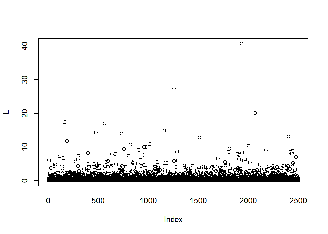
Nonparametric estimates of \(\text{VaR}_\alpha\) and \(\text{ES}_\alpha\) for a fixed \(\alpha\)
alpha = 0.99
(VaR. = VaR_np(L, level = alpha))
## [1] 8.166942(ES. = ES_np(L, level = alpha, verbose = TRUE))## [1] 13.42251plot(L)
abline(h = c(VaR., ES.), lty = 2)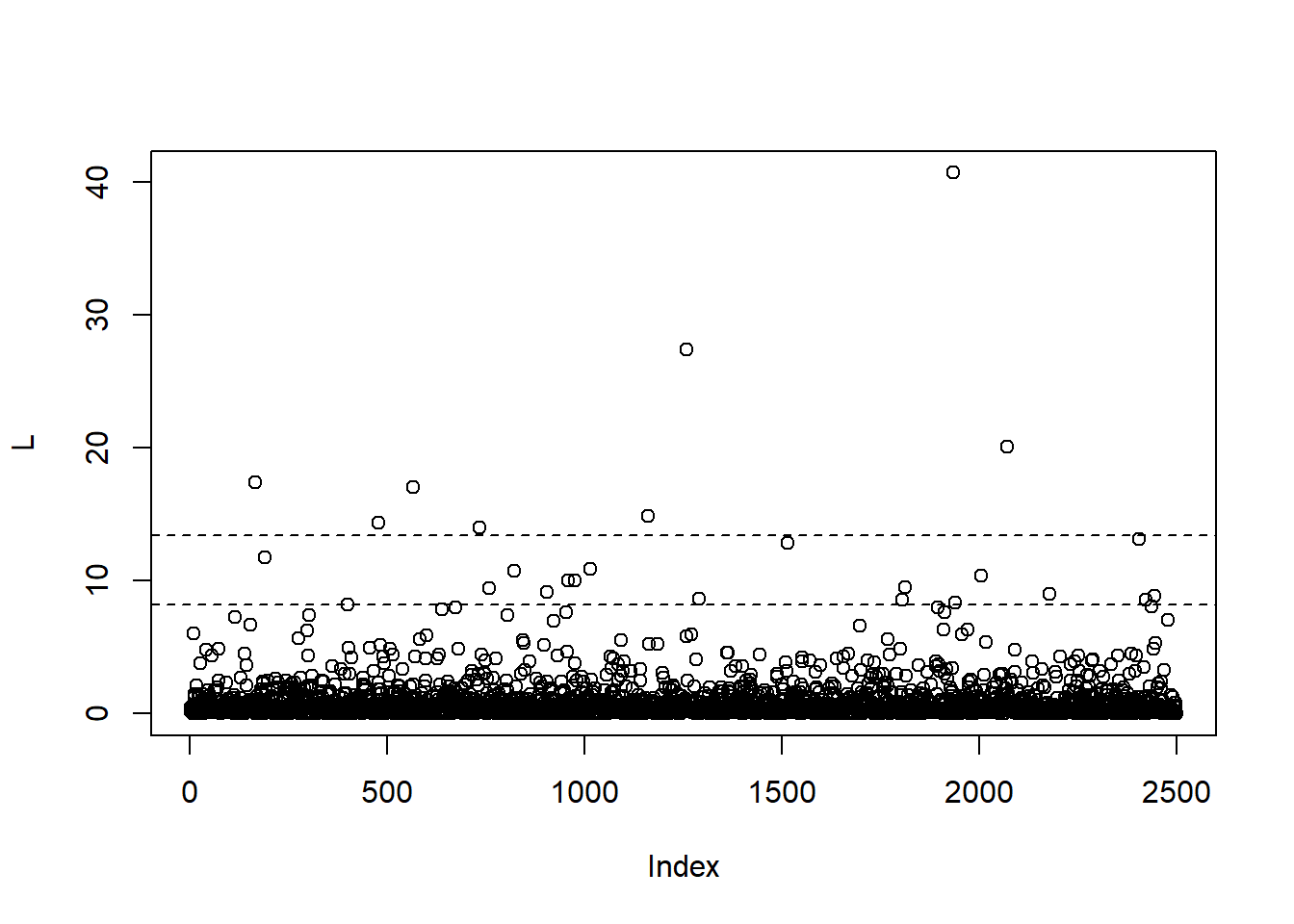
## ... but single numbers don't tell us much
## More interesting: The behavior in alpha
As functions in \(\alpha\) vs true values
Compute the nonparametric \(\text{VaR}_\alpha\) and \(\text{ES}_\alpha\) estimators as functions of \(\alpha\):
alpha = 1-10^-seq(0.5, 5, by = 0.05) # alphas we investigate (concentrated near 1)
stopifnot(0 < alpha, alpha < 1)
VaR. = VaR_np(L, level = alpha) # estimate VaR_alpha for all alpha
suppressWarnings(
   ES.  <-  ES_np(L, level = alpha, verbose = TRUE)
   ) # estimate ES_alpha for all alpha
if(FALSE)
    warnings()
## True values (known here)
VaR.Par. = VaR_Par(alpha, shape = th) # theoretical VaR_alpha values
ES.Par. = ES_Par(alpha, shape = th) # theoretical ES_alpha valuesPlot estimates with true VaR_alpha and ES_alpha values
ran = range(ES.Par., ES., VaR.Par., VaR., na.rm = TRUE)
plot(alpha, ES.Par., type = "l", ylim = ran,
     xlab = expression(alpha),
     ylab = expression("True"~VaR[alpha]*","~ES[alpha]~"and estimates")) # true ES_alpha
lines(alpha, ES., type = "l", col = "maroon3") # ES_alpha estimate
lines(alpha, VaR.Par., type = "l") # true VaR_alpha
lines(alpha, VaR., type = "l", col = "royalblue3") # VaR_alpha estimate
legend("topleft", bty = "n", y.intersp = 1.2, lty = rep(1, 3),
       col = c("black", "maroon3", "royalblue3"),
       legend = c(expression(ES[alpha]~"and"~VaR[alpha]),
                  expression(widehat(ES)[alpha]),
                  expression(widehat(VaR)[alpha])))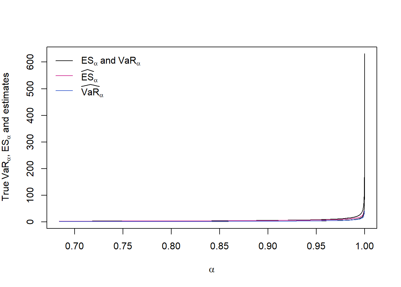
## => We don't see much## With logarithmic y-axis
ran = range(ES.Par., ES., VaR.Par., VaR., na.rm = TRUE)
plot(alpha, ES.Par., type = "l", ylim = ran, log = "y",
xlab = expression(alpha),
ylab = expression("True"~VaR[alpha]*","~ES[alpha]~"and estimates")) # true ES_alpha
lines(alpha, ES., type = "l", col = "maroon3") # ES_alpha estimate
lines(alpha, VaR.Par., type = "l") # true VaR_alpha
lines(alpha, VaR., type = "l", col = "royalblue3") # VaR_alpha estimate
legend("topleft", bty = "n", y.intersp = 1.2, lty = rep(1, 3),
col = c("black", "maroon3", "royalblue3"),
legend = c(expression(ES[alpha]~"and"~VaR[alpha]),
expression(widehat(ES)[alpha]),
expression(widehat(VaR)[alpha])))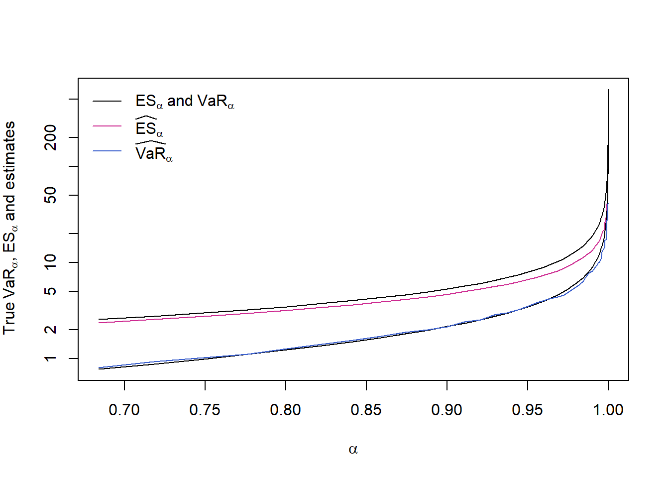
## => We already see that ES_alpha always underestimates its true value
##    (ES_alpha is more difficult to estimate than VaR_alpha)
## With logarithmic x- and y-axis and in 1-alpha
## Note: This is why we chose an exponential sequence (powers of 10) in alpha
## concentrated near 1, so that the x-axis points are equidistant when
## plotted in log-scale)
plot(1-alpha, ES.Par., type = "l", ylim = ran, log = "xy",
xlab = expression(1-alpha),
ylab = expression("True"~VaR[alpha]*","~ES[alpha]~"and estimates")) # true ES_alpha
lines(1-alpha, ES., type = "l", col = "maroon3") # ES_alpha estimate
lines(1-alpha, VaR.Par., type = "l") # true VaR_alpha
lines(1-alpha, VaR., type = "l", col = "royalblue3") # VaR_alpha estimate
legend("topright", bty = "n", y.intersp = 1.2, lty = rep(1, 3),
col = c("black", "maroon3", "royalblue3"),
legend = c(expression(ES[alpha]~"and"~VaR[alpha]),
expression(widehat(ES)[alpha]),
expression(widehat(VaR)[alpha])))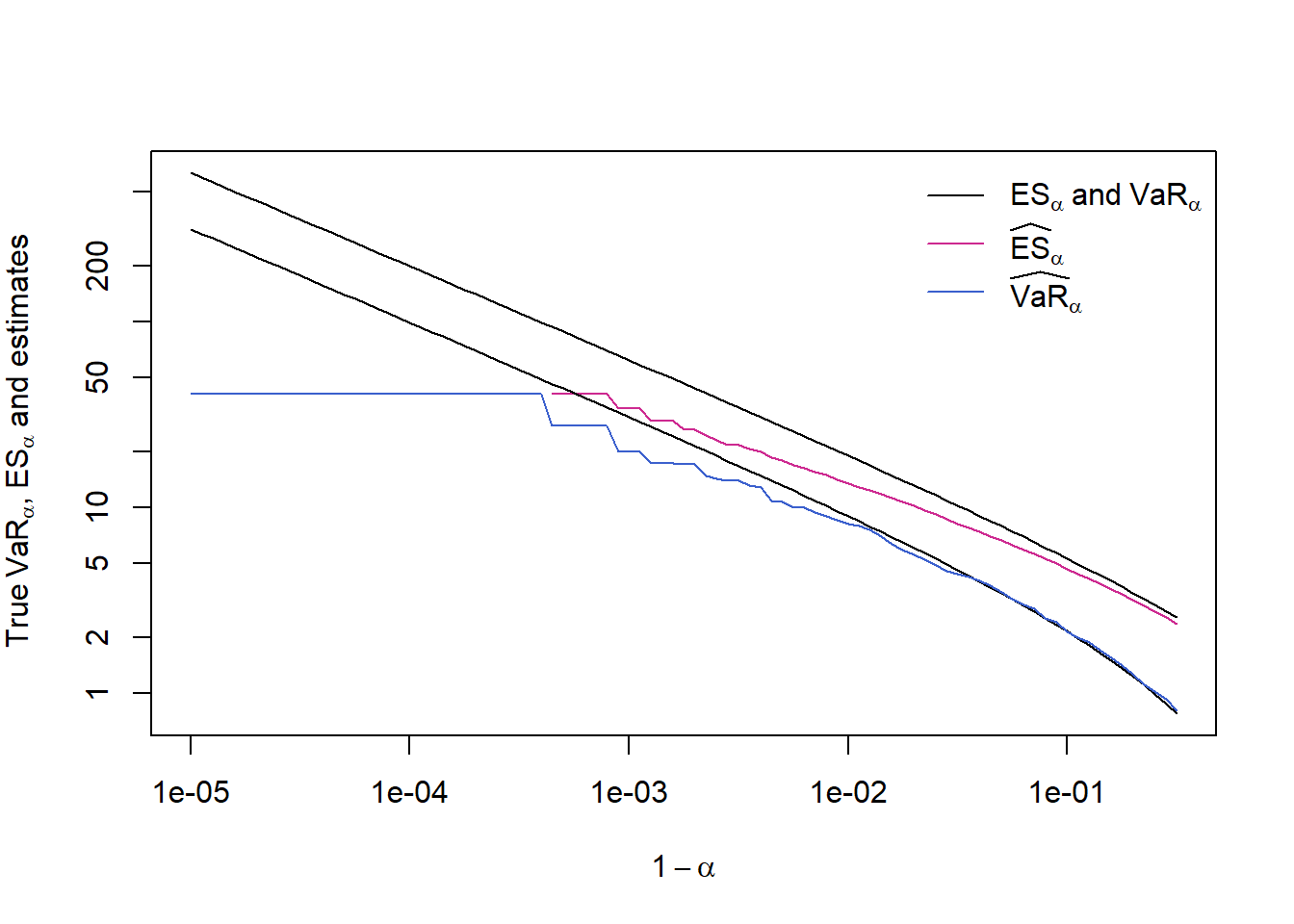
## => - Critical for ES_0.99; severely critical for alpha ~ 0.999.
##    - By using nonparametric estimators we underestimate the risk
##      capital and this although we have comparably large 'n' here!
##    - Note that VaR_alpha is simply the largest max(L) for alpha
##      sufficiently large.
Q: Why do the true \(\text{VaR}_\alpha\) and \(\text{ES}_\alpha\) seem ‘linear’ in \(\alpha\) for large alpha in log-log scale?
A:
Linearity in log-log scale means that \(y\) is a power function in \(x\): \[ y = x^\beta \Rightarrow \log(y) = \beta \cdot \log(x), \] so (\(\log(x)\), \(\log(y)\)) is a line with slope \(\beta\) if \(y = x^\beta\).
For a Pareto distribution, \[ \begin{aligned} \text{VaR}_\alpha(L) &= (1-\alpha)^{-1/\theta} - 1, \\ \text{ES}_\alpha(L) &= (\theta/(\theta-1)) \cdot (1-\alpha)^{-1/\theta} - 1. \end{aligned} \] Omitting the ‘\(-1\)’ for large alpha, we see that \[ \begin{aligned} \text{VaR}_\alpha(L) &\approx (1-\alpha)^{-1/\theta}, \\ \text{ES}_\alpha(L) &\approx (\theta/(\theta-1)) * (1-\alpha)^{-1/\theta} \end{aligned} \] from which it follows that \[ \begin{aligned} (\log(1-\alpha), \log(\text{VaR}_\alpha(L))) &\approx \text{a line with slope } -1/\theta, \\ (\log(1-\alpha), \log(\text{ES}_\alpha(L))) &\approx \text{a line with slope } -1/\theta and intercept \log(\theta/(\theta-1)) \end{aligned} \]
2.3.4 Bootstrapping confidence intervals for \(\text{VaR}_\alpha\), \(\text{ES}_\alpha\)
\(\text{VaR}_\alpha\)
## Bootstrap the VaR estimator
set.seed(271)
VaR.boot = bootstrap(L, B = B, level = alpha) # (length(alpha), B)-matrix containing the bootstrapped VaR estimators
stopifnot(all(!is.na(VaR.boot))) # no NA or NaN
## Compute statistics
VaR.boot. = rowMeans(VaR.boot) # bootstrapped mean of the VaR estimator; length(alpha)-vector
VaR.boot.var = apply(VaR.boot, 1, var) # bootstrapped variance of the VaR estimator; length(alpha)-vector
VaR.boot.CI = apply(VaR.boot, 1, CI) # bootstrapped 95% CIs; (2, length(alpha))-matrix\(\text{ES}_\alpha\)
## Bootstrap the ES estimator
set.seed(271)
suppressWarnings(
   system.time(ES.boot <- bootstrap(L, B = B, level = alpha, method = "ES"))
   ) # (length(alpha), B)-matrix containing the bootstrapped ES estimators
## user system elapsed
## 9.20 0.02 9.32if(FALSE)
warnings()## Investigate appearing NaNs (due to too few losses exceeding hat(VaR)_alpha)
isNaN = is.nan(ES.boot) # => contains some NaN
image(x = alpha, y = seq_len(B), z = isNaN, col = c("white", "black"),
xlab = expression(alpha), ylab = "Bootstrap replication")
mtext("Black: NaN; White: OK", side = 4, line = 1, adj = 0)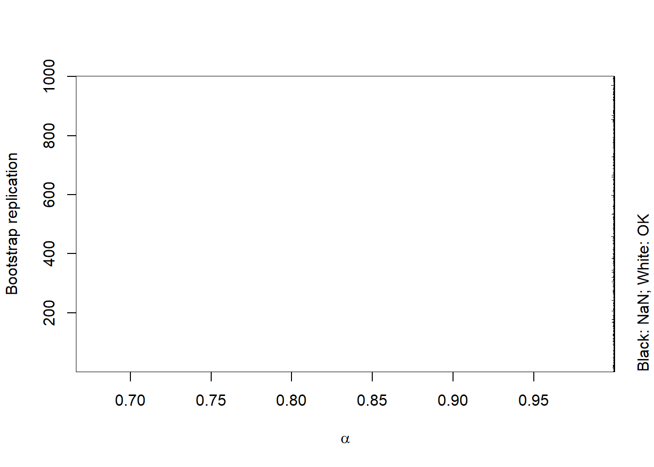
## Plot % of NaN
percNaN = 100 * apply(isNaN, 1, mean) # % of NaNs for all alpha
plot(1-alpha, percNaN, type = "l", log = "x",
     xlab = expression(1-alpha), ylab = expression("% of NaN when estimating"~ES[alpha]))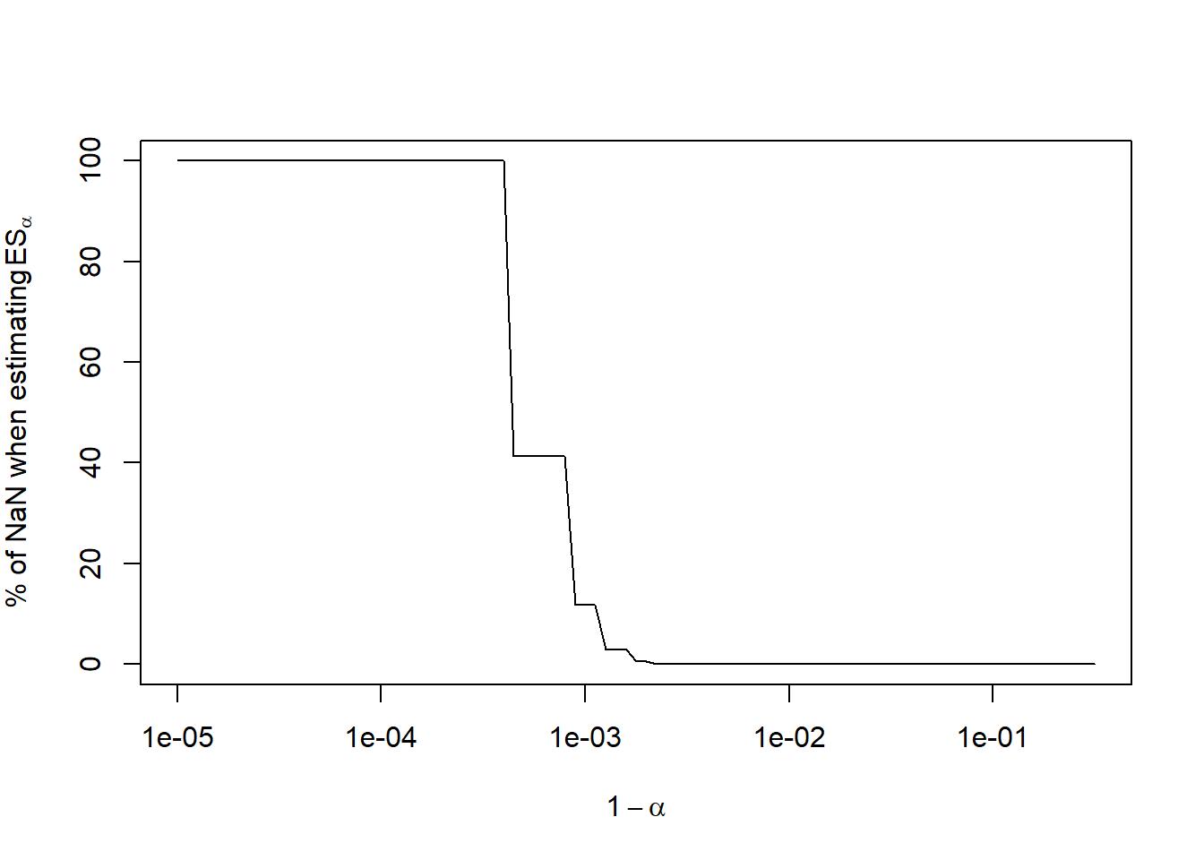
## => Becomes a serious issue for alpha >= 0.999 (1-alpha <= 10^{-3})## Compute statistics with NaNs removed
na.rm = TRUE # only partially helps (if no data available, the result is still NaN)
ES.boot. = rowMeans(ES.boot, na.rm = na.rm) # bootstrapped mean of the ES estimator; length(alpha)-vector
ES.boot.var = apply(ES.boot, 1, var, na.rm = na.rm) # bootstrapped variance of the ES estimator; length(alpha)-vector
ES.boot.CI = apply(ES.boot, 1, CI, na.rm = na.rm) # bootstrapped 95% CIs; (2, length(alpha))-matrix
## => Compute it over the remaining non-NaN values (contains NAs then)2.3.5 Plots
Plot as a function in alpha:
True \(\text{VaR}_\alpha\) and \(\text{ES}_\alpha\)
The nonparametric estimates \(\widehat{\text{VaR}}_\alpha\) and \(\widehat{\text{ES}}_\alpha\)
The bootstrapped mean of \(\widehat{\text{VaR}}_\alpha\) and \(\widehat{\text{ES}}_\alpha\)
The bootstrapped variance of \(\widehat{\text{VaR}}_\alpha\) and \(\widehat{\text{ES}}_\alpha\)
The bootstrapped 95% confidence intervals for \(\text{VaR}_\alpha\) and \(\text{ES}_\alpha\)
ran = range(VaR.Par., # true VaR
             VaR., # nonparametric estimate
             VaR.boot., # bootstrapped estimate (variance Var(VaR.)/B)
             VaR.boot.var, # bootstrapped variance
             VaR.boot.CI, # bootstrapped confidence intervals
             ES.Par., ES., ES.boot., ES.boot.var, ES.boot.CI, na.rm = TRUE) # same for ES_alpha

## VaR_alpha
plot(1-alpha, VaR.Par., type = "l", log = "xy", xaxt = "n", yaxt = "n",
     ylim = ran, xlab = expression(1-alpha), ylab = "") # true VaR_alpha
lines(1-alpha, VaR., lty = "dashed", lwd = 2, col = "royalblue3") # nonparametrically estimated VaR_alpha
lines(1-alpha, VaR.boot., lty = "solid", col = "royalblue3") # bootstrapped nonparametric estimate of VaR_alpha
lines(1-alpha, VaR.boot.var, lty = "dotdash", lwd = 1.4, col = "royalblue3") # bootstrapped Var(hat(VaR)_alpha)
lines(1-alpha, VaR.boot.CI[1,], lty = "dotted", col = "royalblue3") # bootstrapped 95% CI
lines(1-alpha, VaR.boot.CI[2,], lty = "dotted", col = "royalblue3")

## ES_alpha
lines(1-alpha, ES.Par.) # true ES_alpha
lines(1-alpha, ES., lty = "dashed", lwd = 2, col = "maroon3") # nonparametrically estimated ES_alpha
lines(1-alpha, ES.boot., lty = "solid", col = "maroon3") # bootstrapped nonparametric estimate of ES_alpha
lines(1-alpha, ES.boot.var, lty = "dotdash", lwd = 1.4, col = "maroon3") # bootstrapped Var(hat(ES)_alpha)
lines(1-alpha, ES.boot.CI[1,], lty = "dotted", col = "maroon3") # bootstrapped 95% CI
lines(1-alpha, ES.boot.CI[2,], lty = "dotted", col = "maroon3")

## Also adding peaks-over-threshold-based estimators (as motivation for Chapter 5)
u = quantile(L, probs = 0.95, names = FALSE)
L. = L[L > u] - u # compute the excesses over u
fit = fit_GPD_MLE(L.) # fit a GPD to the excesses
xi = fit$par[["shape"]] # fitted shape xi
beta = fit$par[["scale"]] # fitted scale beta
if(xi <= 0) stop("Risk measures only implemented for xi > 0.")
Fbu = length(L.) / length(L) # number of excesses / number of losses = N_u / n
VaR.POT = u + (beta/xi)*(((1-alpha)/Fbu)^(-xi)-1) # see MFE (2015, Section 5.2.3)
ES.POT = (VaR.POT + beta-xi*u) / (1-xi) # see MFE (2015, Section 5.2.3)
lines(1-alpha, VaR.POT, lty = "dashed")
lines(1-alpha, ES.POT,  lty = "dashed")

## Misc
eaxis(1) # a nicer exponential y-axis
eaxis(2) # a nicer exponential y-axis
mtext(substitute(B == B.~~"replications of size"~~n == n.~~"from Par("*th.*")",
                 list(B. = B, n. = n, th. = th)), side = 4, line = 1, adj = 0) # secondary y-axis label
legend("bottomleft", bty = "n", lwd = c(1, rep(c(2, 1, 1.4, 1), 2), 1),
       lty = c("solid", rep(c("dashed", "solid", "dotdash", "dotted"), times = 2), "dashed"),
       col = c("black", rep(c("royalblue3", "maroon3"), each = 4), "black"),
       legend = c(## VaR_alpha
                  expression("True"~VaR[alpha]~"and"~ES[alpha]),
                  expression(widehat(VaR)[alpha]),
                  expression("Bootstrapped"~~widehat(VaR)[alpha]),
                  expression("Bootstrapped"~~Var(widehat(VaR)[alpha])),
                  "Bootstrapped 95% CIs",
                  ## ES_alpha
                  expression(widehat(ES)[alpha]),
                  expression("Bootstrapped"~~widehat(ES)[alpha]),
                  expression("Bootstrapped"~~Var(widehat(ES)[alpha])),
                  "Bootstrapped 95% CIs",
                  ## POT
                  expression("POT-based"~VaR[alpha]~"and"~ES[alpha]~"estimates")))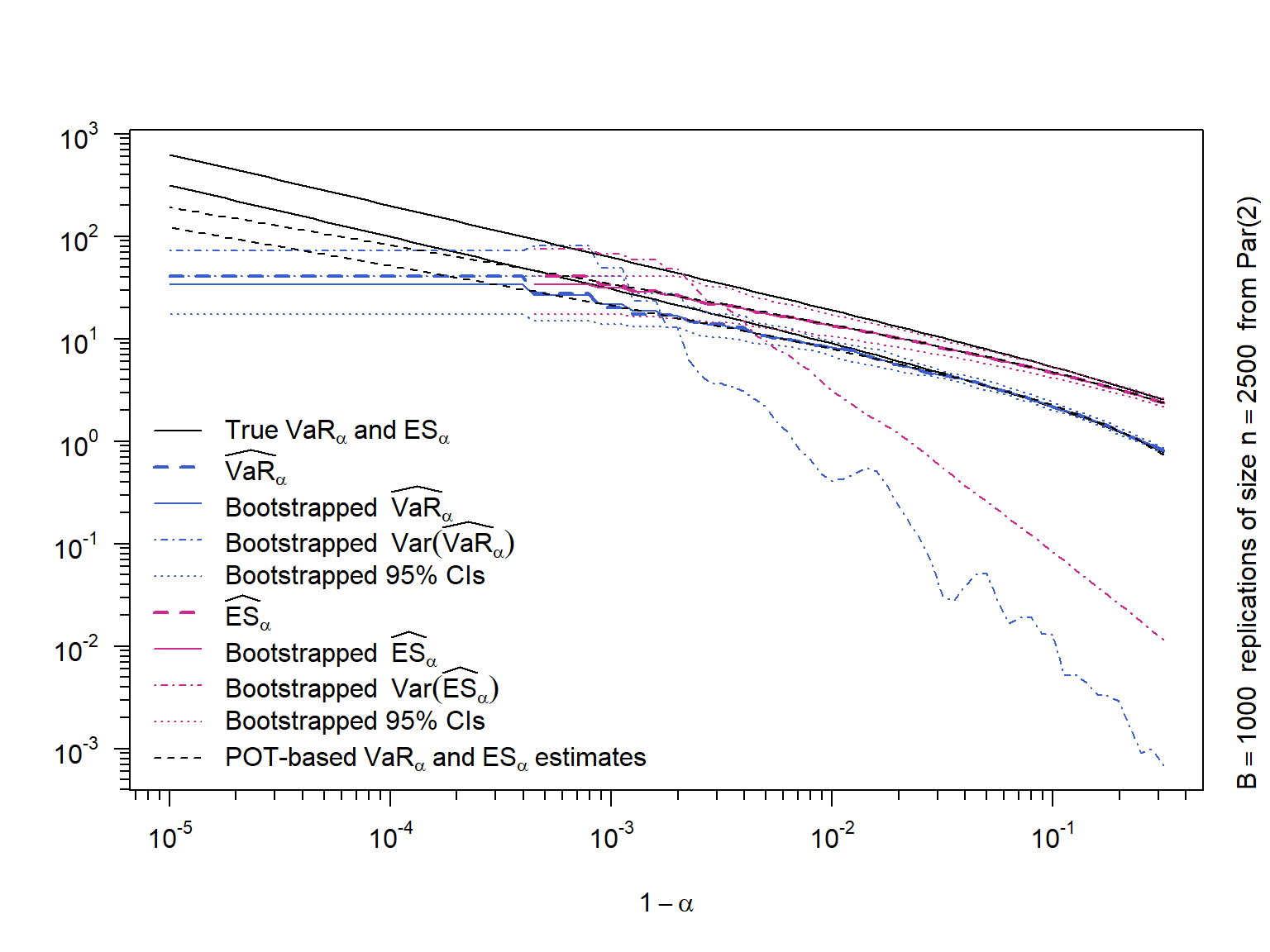
2.3.6 Results
\(\widehat{\text{VaR}}_\alpha < \widehat{\text{ES}}_\alpha\) (clear)
\(\widehat{\text{ES}}_\alpha\) (and bootstrapped quantities) are not available for large \(\alpha\) (there is no observation beyond \(\widehat{\text{VaR}}_\alpha\) anymore)
\(\widehat{\text{VaR}}_\alpha\) and \(\widehat{\text{ES}}_\alpha\) underestimate \(\text{VaR}_\alpha\) and \(\text{ES}_\alpha\) for large \(\alpha\); \(\widehat{\text{ES}}_\alpha\) even a bit more (a non-parametric estimator cannot adequately capture the tail)
\(Var(\widehat{\text{VaR}}_\alpha)\) and \(Var(\widehat{\text{ES}}_\alpha)\) (mostly) increase in \(\alpha\) (less data to the right of \(\text{VaR}_\alpha \Rightarrow\) higher variance)
\(Var(\widehat{\text{ES}}_\alpha) > Var(\widehat{\text{VaR}}_\alpha)\) (\(\widehat{\text{ES}}_\alpha\) requires information from the whole tail)
For not too extreme \(\alpha\), the estimated CI for \(\text{ES}_\alpha\) are larger than those for \(\text{VaR}_\alpha\)
The POT-based method (see later) allows more accurate estimates for large \(\alpha\)
2.4 Exercises
library(sfsmisc) # for eaxis()
library(qrmtools)
options(digits = 10)## Covariance matrices of X
sig.d.1 = 0.2 /sqrt(250)
sig.d.2 = 0.25/sqrt(250)
rho = 0.4
rho. = 0.6
(Sigma = matrix(c(sig.d.1^2, rho *sig.d.1*sig.d.2, rho *sig.d.1*sig.d.2, sig.d.2^2), ncol = 2))## [,1] [,2]
## [1,] 0.00016 0.00008
## [2,] 0.00008 0.00025(Sigma. = matrix(c(sig.d.1^2, rho.*sig.d.1*sig.d.2, rho.*sig.d.1*sig.d.2, sig.d.2^2), ncol = 2))## [,1] [,2]
## [1,] 0.00016 0.00012
## [2,] 0.00012 0.00025## Setup
w = c(0.7, 0.3)
V.t = 10^6
alpha = 0.99
q = qnorm(alpha)
## VaR and ES for rho = 0.4
(VaR.99 = V.t * sqrt(drop(t(w) %*% Sigma %*% w)) * q)## [1] 26979.61825stopifnot(all.equal(VaR.99,
VaR_t(0.99, loc = 0,
scale = V.t * sqrt(drop(t(w) %*% Sigma %*% w)),
df = Inf))) # sanity check
(ES.99 = V.t * sqrt(drop(t(w) %*% Sigma %*% w)) * dnorm(q)/(1-alpha))## [1] 30909.59139stopifnot(all.equal(ES.99,
ES_t(0.99, loc = 0,
scale = V.t * sqrt(drop(t(w) %*% Sigma %*% w)),
df = Inf))) # sanity check
## VaR and ES for rho = 0.6
(VaR.99 = V.t * sqrt(drop(t(w) %*% Sigma. %*% w)) * q)## [1] 28615.0245stopifnot(all.equal(VaR.99,
VaR_t(0.99, loc = 0,
scale = V.t * sqrt(drop(t(w) %*% Sigma. %*% w)),
df = Inf))) # sanity check
(ES.99 = V.t * sqrt(drop(t(w) %*% Sigma. %*% w)) * dnorm(q)/(1-alpha))## [1] 32783.21831stopifnot(all.equal(ES.99,
ES_t(0.99, loc = 0,
scale = V.t * sqrt(drop(t(w) %*% Sigma. %*% w)),
df = Inf))) # sanity checkExercise 2.2 (Basic historical simulation) Consider two stocks, indexed by \(j \in \{1, 2\}\), with current values \(S_{t,1} = 1000\) and \(S_{t,2} = 100\) in some unit of currency. The monthly log-returns of both stocks over the last 10 months are given in the following table (values in %):
| Lag \(k\) | 10 | 9 | 8 | 7 | 6 | 5 | 4 | 3 | 2 | 1 |
|---|---|---|---|---|---|---|---|---|---|---|
| Log-return of \(S_1\) at lag \(k\) | -16.1 | 5.1 | -0.4 | -2.5 | -4 | 10.5 | 5.2 | -2.9 | 19.1 | 0.4 |
| Log-return of \(S_2\) at lag \(k\) | -8.2 | 3.1 | 0.4 | -1.5 | -3 | 4.5 | 2 | -3.7 | 10.9 | -0.4 |
Use historical simulation to estimate the one-month VaR at confidence level \(\alpha = 0.9\) for the linearized loss \(L^\Delta\) for the following two portfolios:
A portfolio consisting of two shares of the first stock \(S_1\).
A portfolio consisting of one share of the first stock and 10 shares of the second stock.
## Monthly log-returns
X.tp1.1 = c(-16.1, 5.1, -0.4, -2.5, -4, 10.5, 5.2, -2.9, 19.1,  0.4) / 100 # X_{t+1,1}
X.tp1.2 = c( -8.2, 3.1,  0.4, -1.5, -3,  4.5, 2,   -3.7, 10.9, -0.4) / 100 # X_{t+1,2}

## a)
(L = -2 * 1e3 * X.tp1.1) # -lambda_1 S_{t,1} X_{t+1,1}
## [1] 322 -102 8 50 80 -210 -104 58 -382 -8(VaR.90.a = quantile(L, probs = 0.9, names = FALSE, type = 1)) # VaR_{0.9}## [1] 80## Note: Changing sort(-X.tp1.1)[9] changes VaR.90.a
## b)
(L = -1 * 1e3 * X.tp1.1 - 10 * 100 * X.tp1.2) # -lambda_1 S_{t,1} X_{t+1,1} - lambda_2 S_{t,2} X_{t+1,2}## [1] 243 -82 0 40 70 -150 -72 66 -300 0(VaR.90.b = quantile(L, probs = 0.9, names = FALSE, type = 1)) # VaR_{0.9}## [1] 70## Note: Changing the second-largest loss of S_1 changes VaR.90.b:
## 1) X.tp1.2[5] = -5 < -4 = X.tp1.1[5] => VaR.90.b = 90 > 80 = VaR.90.a
## 2) X.tp1.2[5] = -4 = X.tp1.1[5] => VaR.90.b = 80 = VaR.90.a
## 3) X.tp1.2[5] = -3 > -4 = X.tp1.1[5] => VaR.90.b = 70 < 80 = VaR.90.a