4 Introduction to simple Linear Regression

Linear regression is a powerful statistical method often used to study the linear relation between two or more variables. It can be seen as a descriptive method, in which case we are interested in exploring the linear relation between variables without any intent at extrapolating our findings beyond the sample data. It can also be seen as an inferential method, in which case we intend to extrapolate our findings from a sample data by making a sweeping general statements about a population of interest. Inference statistics is tricky and requires some understanding of probability theory. Extrapolating our findings from a sample data to the general population of interest is subject to errors, and we use probability theories to quantify these errors, and communicate the uncertainty associated with our findings. Because we haven’t introduced probability theory yet in this class, we will focus on the exploratory aspect of linear regression. We will come back to the inferential aspect of linear regression near the end of the course. Ideally we would introduce linear regression after we have covered probability theory; however, we want to go with the flow started in chapter 3 of the course. Here is the flow I am trying to keep going: the idea of z-score is central to the concept of correlation; the idea of correlation is central to the concept of linear regression. And the scatterplot is central to both the correlation and linear regression ideas.

4.1 Correlation

In section 3.1.1.1, we learned how to draw a scatterplot. We also defined scatterplot as a graphical display of the relationship between two quantitative variables. One variable is shown on the horizontal axis and the other variable is shown on the vertical axis. The observations for the n subjects (or elements) are n points on the scatterplot. The general pattern of the plotted points suggests the overall relationship between the two variables. If we suspect that one variable explains the behavior of the other variable, we should have the explaining variable on the x axis and the response variable on the y axis. By response variable, we mean the explained variable. Once we draw the scatterplot, we can have a good idea of the relationship between the two variables. We often materialize this relationship with a trendline. The easiest interpretation of the trendline would be to say that there is a positive, negative, or no relationship between the two variables. Wouldn’t that be great if we can have a measure of the strength of the relationship? That is what the correlation coefficient does.

4.1.1 Definition

The correlation coefficient measures the direction and strength of the linear relationship between two quantitative variables. The correlation coefficient is usually written as r.

Suppose that we have data on variables $X$ and $Y$ for n individuals. The means and standard deviations of the two variables are $\bar X$ and $s_X$ (for the X variable), $\bar Y$ and $s_Y$ (for the Y variable). The correlation r between $X$ and $Y$ is: \[r = \frac{1}{n-1} \sum^n_i \Bigg (\frac{X_i-\bar X}{s_X} \Bigg ) \Bigg (\frac{Y_i- \bar Y}{s_Y} \Bigg )\] \[i.e.\] \[r = \frac{1}{n-1} \sum^n_i z_{x_i} z_{y_i}\] \[i.e.\] \[r = \frac{1}{n-1} (z_{x_1} z_{y_1} + z_{x_2} z_{y_2} + z_{x_3} z_{y_3}+ ... + z_{x_n} z_{y_n})\]

Question: looking at the formula, when would r be:

Positive
Negative

When looking at a scatterplot, the overall pattern includes: trend, direction, and strength of the relationship. The trend can be linear, curved, or no pattern at all. The direction can be positive, negative or no direction at all. By strength, we refer to how closely the points fit the trend. The figure below shows a few scatterplots and the correlation values:

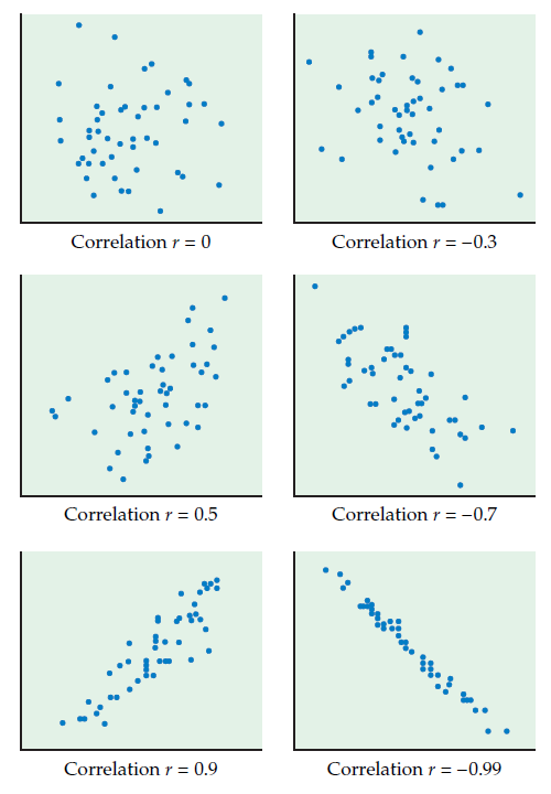
source: Introduction to the Practice of Statistics 6th edition Moore, McCABE, and Craig

4.1.2 Properties of the correlation coefficient

Correlation makes no use of the distinction between explanatory and response variables. It makes no difference which variable you call x and which you call y in calculating the correlation.
Correlation requires that both variables be quantitative, so that it makes sense to do the arithmetic indicated by the formula for r. We cannot calculate a correlation between the incomes of a group of people and what city they live in, because city is a categorical variable (a boxplot of income by city would be a much better tool to use in that case).
Because r uses the standardized values of the observations, r does not change when we change the units of measurement of x, y, or both. Measuring height in inches rather than centimeters and weight in pounds rather than kilograms does not change the correlation between height and weight. The correlation r itself has no unit of measurement; it is just a number.
Positive r indicates positive association between the variables, and negative r indicates negative association.
The correlation r is always a number between $-1$ and $1$. Values of r near 0 indicate a very weak linear relationship. The strength of the relationship increases as r moves away from 0 toward either $-1$ or $1$. Values of r close to $-1$ or $1$ indicate that the points lie close to a straight line. The extreme values $r = -1$ and $r = 1$ occur only when the points in a scatterplot lie exactly along a straight line.
Correlation measures the strength of only the linear relationship between two variables. Correlation does not describe curved relationships between variables, no matter how strong they are.
Like the mean and standard deviation, the correlation is not resistant to outliers: r is strongly affected by a few outlying observations. Use r with caution when outliers appear in the scatterplot.

Example: The table below shows Reed Auto Sales number of TV ads (x) and sales (y). Find the correlation coefficient between the two variables x and y.

Number of TV Ads (x)	Number of Cars Sold (y)
1	14
3	24
2	18
1	17
3	27

Source: Introduction to the Practice of Statistics 6th edition Moore, McCABE, and Craig.

Practice question: Recover the correlation coefficient obtained in page 66 of “Naked Statistics”, by using only the two columns B and C. The goal is for you to convince yourself that you can compute the correlation coefficient by hand.

4.2 Simple linear regression

We have seen how to explore the relationship between two quantitative variables graphically, with a scatterplot. When the relationship has a linear (or straight-line) pattern, the correlation provides a numerical measure of the strength and direction of the relationship. We can analyze the data further by finding an equation for the straight line that best describes that pattern. That equation predicts the value of the response variable from the value of the explanatory variable. The straight line that best describes the linear pattern is called the regression line. The equation of the regression line predicts the value for the response variable y from the explanatory variable x. The equation for the regression line has the form: \[y = a + bx\] Where $a$ denotes the y-intercept, and $b$ denotes the slope.

Regression line

Note: The response variable is also referred as the dependent variable; and the explanatory variable is also referred as the independent variable. The regression is referred as multiple regression when we have two or more independent variables.

A regression equation is often called a prediction equation, since it predicts the value of the response variable y at any value of x.

4.2.1 Interpreting the regression line

Again, in descriptive statistics, the simple linear regression line describes the nature of the relationship between the dependent variable y and the independent variable x. The slope of the line reflects the degree to which the variable y changes linearly as a function of changes in the variable x. The sign of the slope indicates whether the relationship between x and y is positive or negative. A positive slope indicates that both variables changes in the same direction; and a negative slope indicates that x and y changes in opposite directions. If there is no linear relationship between x and y, then the regression line will be flat (zero slope).

Interpreting the slope of the regression line

4.2.2 Estimation of the regression line: the method of least squares

The method of least squares is the most popular method used to calculate the coefficients of the regression line. Recall that the goal of the regression line is to find the line that best describes the linear pattern observed on the scatterplot. The least squares method is the method that minimizes the error terms (also called residuals). The error terms ($\epsilon_i$) are the difference between the observed values of y ($y_i$) and the predicted values of y ($\hat y_i$). The linear model is written as:

\[y_i = a +bx_i + \epsilon_i\]

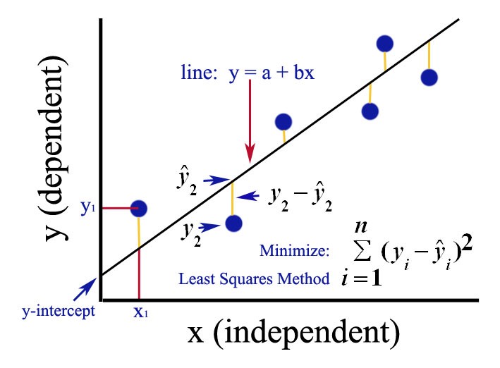
Ordinary least squares plot

The ordinary least squares (OLS) seeks $a$, $b$ to minimize the quantity \[Q(a, b) = \sum^n_i (y_i - \hat y)^2 = \sum^n_i (y_i- (a + bx))^2\]

A simple use of calculus yields the following formulas for $a$ and $b$.

\[a = \bar y - b \bar x\] \[b = \frac{\sum^n_i(x_i - \bar x)(y_i - \bar y)}{\sum^n_i(x_i - \bar x)^2}\]

Note that $b$ can be rewritten as:

\[b = \frac{\frac {1}{n-1}\sum^n_i(x_i - \bar x)(y_i - \bar y)}{\frac {1}{n-1} \sum^n_i(x_i - \bar x)^2} = \frac{cov(x, y)}{var(x)}\]

Where, by definition, $cov(x, y) = \frac {1}{n-1} \sum^n_i (x_i - \bar x)(y_i - \bar y)$

Example: the table below presents data on dollars spent (monthly) for advertisement and the sales recorded.

The scatterplot from these data is:

From the scatterplot above (above), we can say that there is a positive linear relationship between advertising dollars and sales.

And the trend-line (below) indicates the general linear pattern of the data.

Applying our formulas above, we find $a = 28.65$ and $b = 13.9$

Interpretation: a unit increase of advertising dollar increases sales by 13.9 units. Put differently, a dollar increase of advertising money increases sales by $13.9.

The intercept is 28.65, which means that with zero advertising dollars, sales are 28.65 (thousands).

With this regression equation ($\hat y = 28.65 + 13.9x$), we can predict the sales given particular dollars spent on advertisement. Note that x stands for advertising dollars and y stands for sales. So, with this equation, we can predict sales for any level of advertising dollars.

Practice question 1: The table below shows Reed Auto Sales number of TV ads (x) and sales (y). Find the regression line.

Number of TV Ads (x)	Number of Cars Sold (y)
1	14
3	24
2	18
1	17
3	27

4.2.3 Correlation and the simple linear regression

So far, we have alluded that scatterplot, correlation, and simple linear regression are related. By definition, the simple linear regression equation provides us with the best trendline we want to draw on the scatterplot. However, how is the correlation related to the simple linear regression equation? The relation resides in the slope of the regression equation. In fact, it turned out that by playing around with formula of the slope of the regression line, we can find the following relationship between the slope of the regression line (b) and the correlation between the two variables (r). Here is the relationship:

\[b = r \frac{s_y}{s_x}\]

and since $a = \bar y - b \bar x$, we can see that the intercept a is also a function of the correlation (r).

Interpretation: $b = r \frac{s_y}{s_x}$ says that, along the regression line, a change of one standard deviation in x corresponds to a change of r standard deviations in y. Note that the absolute value of the slope increases with the absolute value of the correlation coefficient.

The square of the correlation coefficient, refers as the coefficient of determination, has a particular meaning in linear regression. It tells how much of the variations in y is explained by the variation on x.

Definition: The square of the correlation, $r^2$ , is the fraction of the variation in the values of $y$ that is explained by the variation in $x$.

Why do we interpret $r^2$ the way we interpret it?

The total variations of $y$ ($\sum^n_i(y_i - \bar y)^2$) is due to the variation explained by the regression line ($\sum^n_i(\hat y_i - \bar y)^2$) and some unexplained variations ($\sum^n_i(y_i - \hat y)^2$). That is,

\[\sum^n_i(y_i - \bar y)^2 = \sum^n_i(\hat y_i - \bar y)^2 + \sum^n_i(y_i - \hat y)^2\] \[i.e.\] \[SST = SSR + SSE\]

where,

SST = total sum of squares;

SSR = sum of squares due to the regression

SSE = sum of squares due to the errors

By definition, $r^2 = \frac{SSR}{SST}$

For our sales example, if $r^2 = 0.79$, we would say that 79% of the variations in sales are explained by the variations on advertisement spending.

Practice: For the advertizing and sales data, compute the following:

The standard deviations $s_x$ and $s_y$
The correlation coefficient $r$
The coefficients $a$ and $b$ of the regression line.
Interpret $a$ and $b$
Interpret $r^2$

Sources:

http://www2.cedarcrest.edu/academic/bio/hale/biostat/session24links/regression-assumptions.html
https://onlinecourses.science.psu.edu/stat100/node/37
http://ci.columbia.edu/ci/premba_test/c0331/s7/s7_6.html

4.3 Linear Regression Using R

In practice, we will use a statistical software to compute the coefficients of the regression line.

The lm() function in R does the calculations for us. The following R code illustrates the use of the lm() function. lm stands for linear model.

lm(y~x, data = my_dataframe)

1- Replace y with your outcome (or explained, or dependent) variable.
2- Replace x with your predictor (or explanatory, or independent) variable.
3- Replace my_dataframe with your dataset name.

Keeping with our running example, which uses data on ads and sales, here is an application of the lm() function:

4.3.1 Constructing a dataset

ad <- c(1, 3, 2, 1, 3) # Ads variable
sales <- c(14, 24, 18, 17, 27) # Sales variable
car_dat <- data.frame(Number_of_TV_Ads_x = ad,
                      Number_of_Cars_Sold_y = sales) # combine both into a single dataset (or dataframe)
car_dat # outputs the data

##   Number_of_TV_Ads_x Number_of_Cars_Sold_y
## 1                  1                    14
## 2                  3                    24
## 3                  2                    18
## 4                  1                    17
## 5                  3                    27

4.3.2 A simple use of the `lm()` function

lm(sales~ad, data = car_dat)

## 
## Call:
## lm(formula = sales ~ ad, data = car_dat)
## 
## Coefficients:
## (Intercept)           ad  
##          10            5

4.3.3 A more useful way of using the `lm()` function

By running lm(y~x, data = my_dataframe), R outputs the coefficients for us. However, we get more informations by giving the results a name, and using the summary() function with the name given. Below is an illustration of a good way to use the lm() function.

m1 <- lm(sales~ad, data = car_dat) # gives your results a name
summary(m1) # provides a detailled results

## 
## Call:
## lm(formula = sales ~ ad, data = car_dat)
## 
## Residuals:
##  1  2  3  4  5 
## -1 -1 -2  2  2 
## 
## Coefficients:
##             Estimate Std. Error t value Pr(>|t|)  
## (Intercept)   10.000      2.366   4.226   0.0242 *
## ad             5.000      1.080   4.629   0.0190 *
## ---
## Signif. codes:  0 '***' 0.001 '**' 0.01 '*' 0.05 '.' 0.1 ' ' 1
## 
## Residual standard error: 2.16 on 3 degrees of freedom
## Multiple R-squared:  0.8772, Adjusted R-squared:  0.8363 
## F-statistic: 21.43 on 1 and 3 DF,  p-value: 0.01899

Note that the table under coefficient provides additional information besides the coefficients. These information are the Std. Error, t value, Pr(>|t|) also called p-value. These elements are used to assess the strengh of the linear relation between the $y$ and $x$ variables. We will come back to these elements after we introduce some probability concepts. For now, just accept on faith that:
1- a $p-value \le .10$ suggests a fairly strong relationship between $y$ and $x$.
2- a $p-value \le .05$ suggests a strong relationship between $y$ and $x$.
3- a $p-value \le .01$ suggests a highly strong relationship between $y$ and $x$.

In statistical parlance, we use the phrase statistically significant, to mean strong relationship.

The $r^2$ is also provided, under the name Multiple R-squared, next to the last line of the output.

This is the end of the chapter on simple linear regression. Next, we will extend it with more explanatory variables.