5 Basics of Probability

Descriptive statistics and Inference Statistics are the two biggest aspects of statistics. In order to do inference statistics, it is necessary to have a good understanding of probability. In fact, going from a random sample of a population to a generalization about the population involve uncertainties. For instance, is the sample at hand a good representation of the population? If we had a different sample, would we still have the same descriptive statistics? It is highly likely that different samples will provide different descriptive statistics. So, when we generalize from a sample, there is a chance that we may be making errors. Now, can we have a measure of that probable error? This is when probability comes in in a statistics class.

5.1 Basic probability concepts

5.1.1 Randomness

Toss a coin, or roll a die. Can you predict the results? No! We can nonetheless reasonably guess how likely head or tail will occur; and how likely 1, 2, … , or 6 will occur when a die is rolled. Our guess is particularly true if we repeat the experiment several times. Why? Definitions: We call a phenomenon random if individual outcomes are uncertain but there is nonetheless a regular distribution of outcomes in a large number of repetitions. The probability of any outcome of a random phenomenon is the proportion of times the outcome is expected to occur in a very long series of repetitions.

Fair: A coin or a die is said to be fair if the probability of every side is equally likely.

5.1.2 Probability Models

A description of a random phenomenon in the language of mathematics is called a Probability Model. The study of probabilities consists of assigning probabilities to random phenomena. For instance, when we toss a coin, we cannot predict the outcome, but we can say that the outcome will be either head or tail. Moreover, if we know that the coin is a fair coin, we believe that each of these outcomes has probability of 1/2.

The description of coin tossing has two parts:

List of possible outcomes;
A probability for each outcome.

This two-part description is the starting point for a probability model. We will begin by describing the outcomes of a random phenomenon and then learn how to assign probabilities to the outcomes.

5.1.2.1 Sample Spaces

A probability model first tells us what outcomes are possible. The sample space S of a random phenomenon is the set of all possible outcomes.

Examples:

1- Sample Space for tossing a coin: $S = \{Head, Tail\} = \{H, T\}$

2- Sample Space for random digits: $S = \{0, 1, 2, 3, ..., 9\}$

3- Sample Space for rolling a die: $S = \{1, 2, 3, 4, 5, 6\}$

4- A student is asked on which day of the week he or she spends the most time studying. What is the sample space? $S = \{Mon, Tue, Wed, Thr, Fri, Sat, Sun\}$

5- Sample space for heights. You record the height in feet of a randomly selected college student. What is the sample space? $S = [2, 8.5]$ is a sensible guess.

6- Sample Space for tossing a coin four time: \[S = \{HHHH, HHHT, HHTH, HHTT, HTHH, HTHT, \\ HTTH, HTTT, THHH, THHT, THTH, THTT, TTHH, \\ TTHT, TTTH, TTTT\}\]

The tree diagram is often helpful when trying to identify the different outcomes. Below is the tree diagram for identifying the possible outcomes when a coin is tossed four times.

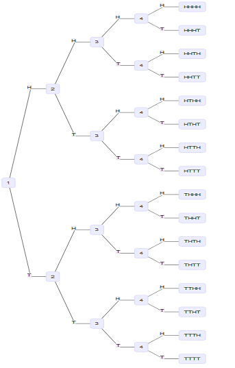
Tree Diagram

A sample space $S$ lists the possible outcomes of a random phenomenon. To complete a mathematical description of the random phenomenon, we must also give the probabilities with which these outcomes occur.

Sometimes, we may want to assign probabilities not only to single outcomes but also to sets of outcomes. An event is an outcome or a set of outcomes of a random phenomenon. That is, an event is a subset of the sample space.

Example: Consider our example of tossing a coin four times. Possible events are: exactly one head (call it event A); exactly two heads (call it event B); exactly three heads (call it event C); exactly four heads (call it event D).

The event B expressed as a set of outcomes is: \[B = \{HHTT, HTHT, HTTH, THHT, THTH, TTHH\}\]

For a toss of a single coin, the outcome head is an event (call it A); $A = {Head}$

5.1.2.2 General facts about probabilities

Any probability is a number between 0 and 1. A probability is a proportion, and any proportion is a number between 0 and 1, so any probability is also a number between 0 and 1. An event with probability 0 never occurs, and an event with probability 1 occurs on every trial. An event with probability 0.5 occurs in half the trials in the long run.
All possible outcomes together must have probability 1. Because every trial will produce an outcome, the sum of the probabilities for all possible outcomes must be exactly 1. Understand the sum of all proportion should add up to one.
If two events have no outcomes in common, the probability that one or the other occurs is the sum of their individual probabilities. If one event occurs in 40% of all trials, a different event occurs in 25% of all trials, and the two can never occur together, then one or the other occurs on 65% of all trials because 40% + 25% = 65%.
The probability that an event does not occur is 1 minus the probability that the event does occur. If an event occurs in (say) 70% of all trials, it fails to occur in the other 30%. The probability that an event occurs and the probability that it does not occur always add to 100%, or 1.

5.1.2.3 Probability rules

If $A$ is any event, we write its probability as $P(A)$.

Formally (or mathematically), facts 1 through 4 can be written as:

Rule 1: The probability $P(A)$ of any event $A$ satisfies $0\le P(A) \le 1$.

Rule 2: If $S$ is the sample space in a probability model, then $P(S) = 1$.

Rule 3: Two events $A$ and $B$ are disjoint if they have no outcomes in common and so can never occur together. If $A$ and $B$ are disjoint, \[P(A \ or \ B) = P(A) + P(B)\]

This is the addition rule for disjoint events.

Rule 4: The complement of any event $A$ is the event that $A$ does not occur, written as $A^c$. The complement rule states that: \[P(A^c) = 1 - P(A)\]

It may be helpful to picture the ideas of disjoint and complement events using a Venn diagram. Let’s assume the rectangles below are our sample space, and that $A$ and $B$ are events in the sample space. $A$ and $B$ do not overlap; thus, they are disjoint. The complement of A ($A^c$) is everything in the sample space $S$, that is, the whole rectangle, except A itself.

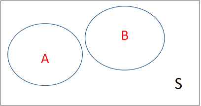
Venn diagram for disjoint events

Example 1: Cell phones and accidents. Some states are considering laws that will ban the use of cell phones while driving because they believe that the ban will reduce phone-related car accidents. One study classified these types of accidents by the day of the week when they occurred. For this example, we use the values from this study as our probability model. Here are the probabilities:

Day	Sun	Mon	Tue	Wed	Thr	Fri	Sat
Probility	0.03	0.19	0.18	0.23	0.19	0.16	0.02

Questions:

Is this probability model a legitimate probability model? Justify your answer.
What is the probability that an accident occurs on a weekend, that is, Saturday or Sunday?
What is the probability that a phone-related accident occurs on a weekday?
Find the probability that a phone-related accident occurred on a Monday or a Friday.
Find the probability that a phone-related accident occurred on a day other than a Wednesday.

Example 2: Benford’s law. Faked numbers in tax returns, payment records, invoices, expense account claims, and many other settings often display patterns that aren’t present in legitimate records. Some patterns, like too many round numbers, are obvious and easily avoided by a clever crook. Others are more subtle. It is a striking fact that the first digits of numbers in legitimate records often follow a distribution known as Benford’s law. Here it is (note that a first digit can’t be 0)

First digit	1	2	3	4	5	6	7	8	9
Probability	0.301	0.176	0.125	0.097	0.079	0.067	0.058	0.051	0.046

Investigators can detect fraud by comparing the first digits in records such as invoices paid by a business with these probabilities.

Questions:

Verify that the Benford’s law is indeed a legitimate probability model.
Consider the events A= {first digit is 1}, and B = {first digit is 6 or greater}; Compute P(A), and P(B).
What is the probability that the first digit is greater than 6?
Find the probability that a first digit is anything other than 1.
Find the probability that a first digit is either 1 or 6 or greater.

5.1.2.4 Assigning probability to equally likely outcomes

If a random phenomenon has $k$ possible outcomes, all equally likely, then each individual outcome has probability $1/k$. The probability of any event $A$ is: \[P(A) = \frac{Counts \ of \ outcomes \ in \ A}{Counts \ of \ outcomes \ in \ S}\]

Example 3: Possible outcomes for rolling a die. A die has six sides with 1 to 6 “spots” on the sides. (1) Give the probability distribution (or probability model) for the six possible outcomes that can result when a perfect die is rolled. (2) Let $A$ be the event the outcome is an even number. Find $P(A)$. (3) Find $P(A^c)$.

5.1.2.5 Independence and multiplication rule

Probability Rule 5: Two events $A$ and $B$ are independent if knowing that one occurs does not change the probability that the other occurs. If $A$ and $B$ are independent, \[P(A \ and \ B) = P(A)P(B)\]

This is the multiplication rule for independent events.

Example 4: Tossing a coin two times. The event $A=\{head \ in \ the \ first \ time\}$, and $B=\{head \ in \ the \ second \ time\}$ are independent. Consequently, \[P(A \ and \ B) = P(A)P(B)\]

Example 5: Dependent events in cards. The colors of successive cards dealt from the same deck are not independent. A standard 52-card deck contains 26 red and 26 black cards. For the first card dealt from a shuffled deck, the probability of a red card is 26/52 = 0.50 because the 52 possible cards are equally likely. Once we see that the first card is red, we know that there are only 25 reds among the remaining 51 cards. The probability that the second card is red is therefore only 25/51 = 0.49. Knowing the outcome of the first deal changes the probabilities for the second.

Practice: The probability of a second ace. A deck of 52 cards contains 4 aces, so the probability that a card drawn from this deck is an ace is 4/52. If we know that the first card drawn is an ace, what is the probability that the second card drawn is also an ace? Using the idea of independence, explain why this probability is not 4/52.

Sources: Introduction to the Practice of Statistics, Sixth Edition, by Moore, McCabe, and Craig, Publisher: W. H. Freeman.

5.2 Additional Probability Rules

5.2.1 General addition rule

Recall that we said that if A and B are disjoint events, then:

\[P(A \ or \ B) = P(A) + P(B)\]

We illustrated that fact with this venn diagram:

Disjoint events A and B

Now considering the following ven diagram where A and B are no longer disjoint, what is the probability of $P(A \ or \ B)$

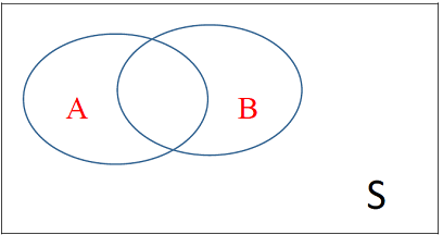
Events A and B are not disjoint

$P(A \ or B) =$

This formula is often referred as the “general addition rule”.

Notation: Mathematically, $(A \ or \ B)$ is written as $A \cup B$, and (A and B) is written as $A \cap B$

So, \[P(A \ or \ B) = P(A \cup B)\]

Definition:

1- The union of any collection of events is the event that at least one of the collection occurs.
2- The intersection of any collection of events is the event that all of the events occur.

Example1: If you roll a die, the probability of each of the six possible outcomes (1, 2, 3, 4, 5, 6) is 1/6.
(a) What is the probability that you roll a 3 or a 5?
(b) What is the probability that your roll is even or greater than 4?

$X = x_i$	1	2	3	4	5	6
$P(X = x_i)$	1/6	1/6	1/6	1/6	1/6	1/6

Answer:

Let A be the event “roll 3 or 5”, B be the event “the roll is even”, and C the event “the roll is greater than 4”. Then,

P(A) =
P(B) =

5.2.2 Conditional Probability

Recall that two events A and B are independent if the probability of A happening does not affect the probability of B happening (and vice versa). We say $P(B\ given \ A) = P(B)$, or $P(A \ given \ B)= P(A)$. Put differently, knowing that B has happened will not change the probability of A happening.
Notation: we use the symbol “|” to mean “given”. Thus $P(B \ given \ A) = P(B|A)$.
Now, let’s use one of our previous practice questions to motivate the formula of conditional probability.

A deck of 52 cards contains 4 aces, so the probability that a card drawn from this deck is an ace is 4/52. If we know that the first card drawn is an ace, what is the probability that the second card drawn is also an ace?

Let’s define A the event “the first card drawn is an ace”, and B “the second card drawn is also an ace”. Two scenarios emerge.

1- With replacement, $P(B|A) = P(B) = 4/52$, and $P(A \ and \ B) = P(A)*P(B|A) = P(A)*P(B)$

Knowing A does not change the probability for B: $P(B|A) = P(B)$

2- Without replacement, $P(B|A)= 3/51$, and $P(A \ and \ B)= P(A)*P(B|A)$

Here, knowing A alters the probability for B: $P(B|A) \not= P(B)$

Aside: Recall that, in probabilistic language, the “or” implies an addition and the “and” implies a multiplication. Thus, the probability of two events C and D is $P(C \ and \ D) = P(C)*P(D)$.

\[P(A \cap B) = P(A)*P(B | A)\] \[P(A)*P(B | A) = P(A \cap B)\] \[P(B | A) = \frac {P(A \cap B)}{P(A)}\]

The formula (1) is known as the multiplication rule, and the formula (2) is known as the conditional probability rule.

Additional resource: http://www.mathsisfun.com/data/probability-events-conditional.html

5.3 Random Variables

When we toss a coin four times, we can record the outcome as a string of heads and tails, such as $HTTH$. In statistics, however, we are most often interested in numerical outcomes such as the count of heads in the four tosses. For convenience, let’s use a shorthand notation; let $X$ be the number of heads. If our outcome is $HTTH$, then $X = 2$. If the next outcome is $TTTH$, the value of X changes to $X = 1$. The possible values of $X$ are $0, 1, 2, 3, \ and \ 4$.

Definition: A random variable is a numerical description of the outcome of an experiment.

Note: We usually denote random variables by capital letters near the end of the alphabet, such as $X$, $Y$, or $Z$.

If $X$ denotes our random variable, we usually list the possible outcomes as: $X= {x_1, x_2, x_3, …}$. For the example of tossing a coin four times, and defining $X$ as the number of heads obtained, $X= {0, 1, 2, 3, 4}$.

We can distinguish two types of random variables: Discrete random Variables, and Continuous random variables.

5.3.1 Discrete Random Variables

A discrete random variable $X$ has a finite number of possible values. Discrete random variables are usually (but not necessarily) counts.

Examples: The number of children in a family, the number of defective light bulbs in a box of ten, the number of car accidents per day in a city, etc.

The probability distribution (or probability model) of X lists the possible values and their probabilities:

Values of X	$x_1$	$x_2$	$x_3$	…	$x_k$
Probability	$p_1$	$p_2$	$p_3$	…	$p_k$

Example1: Number of heads in four tosses of a coin. What is the probability distribution of the discrete random variable X that counts the number of heads in four tosses of a coin?

Values of X	0	1	2	3	4
Probability

Note: We can use histograms to show probability distributions.

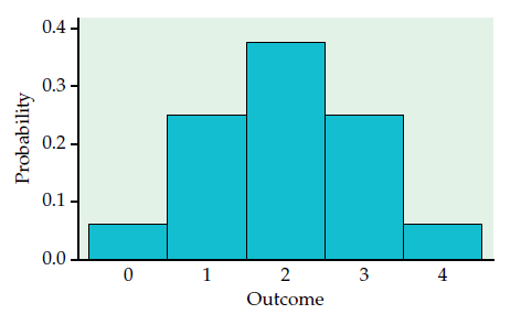
Probability histogram for the number of heads in four tosses of a coin.

Example 1 continued: Using the probability distribution in example 1, find:

The probability of getting at least 3 heads,
The probability of getting at least 2 heads,
The probability of getting at most 2 heads,
The probability of getting at most 3 heads.

Practice: Two tosses of a fair coin. Find the probability distribution for the number of heads that appear in two tosses of a fair coin.

5.3.2 Continuous Random Variables

Definition: A continuous random variable may assume any numerical value in an interval or collection of intervals. Experimental outcomes based on measurement such as time, weight, distance, and temperature can be described by continuous random variables.

Example: Arrival time. Econ 215 start at 2:00 PM; Assuming that the students can get access to the classroom starting from 1:50 PM to 2 PM, the arrival time of any student in the class is between 0 and 10 mn. The student arrival time is zero if he/she enters the classroom at exactly 1:50, and 10 mn if he/she enters the classroom at exactly 2PM. So, the random variable X assumes values between 0 and 10.

5.3.3 The Normal Distribution

Of all the resources I have looked at, the following link provides a very good presentation of the Normal Distribution topic. So, consider this material as part of your notes: http://www.mathsisfun.com/data/standard-normal-distribution.html

The following link provides a short history of the normal distribution:

http://onlinestatbook.com/2/normal_distribution/history_normal.html

Sources: Introduction to the Practice of Statistics, Sixth Edition, by Moore, McCabe, and Craig, Publisher: W. H. Freeman. (p.258-270)

http://www.stat.yale.edu/Courses/1997-98/101/ranvar.htm

5.4 Expected Value and Variance

5.4.1 Expected Value

Assume we have the following series of numbers denoted $X = x_1, x_2, ...x_k$:

$x_1$	$x_2$	$x_3$	$x_4$	$x_5$	$x_6$
$-2$	$-2$	$-2$	$3$	$4$	$4$

What is the mean value $\bar X$?

\[ \bar X = \]

Another way of computing the same mean is:

\[\bar X = \]

This is called the weighted mean. The weights are:

Now, assume a game in which you pay $\$2$ to participate. The game consists of tossing a die. If the die falls on 1, 2, or 3, you lose your $\$2$. If the die falls on 4, you win $\$5$; and you win $\$6$ if the die falls on 5, or 6. Construct the probability model of the random variable X, winning (by winning, we mean net gain here).

Compute the weighted mean of winning:

Note 1: the weighted mean is called Expected Value (in the context of probability model). Its formula is:

\[\mu = E(X) = \bar X = \sum_i p_ix_i\]

Note 2: Like the average number of children does not have to be a whole number, the expected value of a random number does not have to be a value the random variable can assume.

Example: The probability distribution for damage claims paid by Newton Automobile Insurance Company on collision insurance follows (for any given client):

Payment ($), or $X = x_i$	Probability, or $P(X = x_i)$	$x_iP(X = x_i)$	Net receipt by policy holder $Y = y_i$	$y_iP(Y = y_i$
0	0.85
500	0.04
1000	0.04
3000	0.03
5000	0.02
8000	0.01
10000	0.01
Totals	1

Use the expected collision payment to determine the collision insurance premium that would enable the company to break even.
The insurance company charges an annual rate of $520 for collision coverage. What is the expected value of the collision policy for a policy holder? Why does this policy holder purchase a collision policy with this expected value?

5.4.2 Variance

The variance is by definition a measure of dispersion or spreadness. The variance of a random variable $X$ is given by the formula:

\[\sigma^2 = \sum_i p_i (x_i - \mu)^2\] where $p_i$ is the probability of observing $x_i$

Example: Compute the variance of the insurance example above:

Payment ($), or $X = x_i$	Probability, or $P(X = x_i)$	$x_iP(X = x_i)$	$(x_i-\mu)^2$
0	0.85
500	0.04
1000	0.04
3000	0.03
5000	0.02
8000	0.01
1000	0.01
Totals	1	$\mu = 430$	–

There is a simpler formula for the variance: \[\sigma^2 = \sum_i p_i x_i^2 - \mu^2\]

Practice: use the $\sigma^2 = \sum_i p_i x_i^2 - \mu^2$ formula to recover the answer found above, i.e. the answer on the table.