7 Inference for Numerical Data
At the heart of statistics is the desire to understand differences. For instance, is a given drug more effective than a placebo? Do undergraduate students in private schools have more student loans than undergraduate students in public schools? Note that these two questions are about finding if two groups are different in a “meaningful way” with respect to a criterion. Answering to these types of questions is often referred as significance testing, or hypothesis testing. We use significance testing to make a judgment about a claim. The claim is referred as the null hypothesis.
7.1 Hypothesis Testing
Hypothesis testing refers to the formal procedures used by researchers to accept or reject statistical hypotheses. A statistical hypothesis is a claim about the population parameter. For example, we may claim that the population mean is equal to a particular value; Or the population means of two different groups are equal. The claim may be true or false. The task of the researcher is to use sample data to assess the likelihood of the hypothesis (claim) being true. If the sample data is not consistent with the statistical hypothesis, the hypothesis is rejected. There are two types of statistical hypotheses:
- Null hypothesis. The null hypothesis, denoted by \(H_0\), is usually our claim.
- Alternative hypothesis. The alternative hypothesis is denoted by \(H_1\) or \(H_a\).
Note: The test of significance is designed to assess the strength of the evidence against the null hypothesis. Usually the null hypothesis is a statement of “no effect” or “no difference”. For example, when comparing two means, our null hypothesis is:
\(H_0\): there is no difference in the means
\(H_a\): there is a difference in the means
Hypotheses are formulated in such a way that the alternative statement is what we are trying to prove with our test.
We reject the null, \(H_0\) if the evidences in the data are overwelming against the null. By overwelming, we mean to say that the null is very unlikely.
7.2 Steps for hypothesis testing
Researchers follow a formal process to determine whether to reject a null hypothesis, based on sample data. This process, called hypothesis testing, can be summarized in the following 5 steps:
State the research question: stating the research question clearly is necessary in order to define the type of data that should be used.
For example: Is the mean “first salary” of newly graduated students (in Nebraska) equal to $30,000?Formulate the hypotheses: state the research question in terms of null hypothesis \(H_0\) and the alternative hypothesis \(H_a\).
The null hypothesis is the population parameter,$ = $30,00$ (\(H_0: \mu = \$30,000\)). The alternative hypothesis is the population parameter does not equal \(30,000 (\)H_a: = $30,000$). These statements are written as: \[H_0: \mu = \$30,000\] \[H_a: \mu \not = \$30,000\]
- Calculate the test statistics. There are several test statistics. We will look at the z-statistics, also called the z-score. Note that, from a sample data, we can compute the sample mean, which we will compare with the hypothesized parameter µ. Thus the z-statistics is as follows: \[|z^*| = |\frac{\bar X - \mu(hypothesized)}{s/\sqrt n}|\]
Technically the formula of the z-score above is called t-statistics because of the use of s instead of sigma. The z-statistcs, and t-statistics are different when the data size is too small. But they are identical when the data size is “large”. In today’s world, where data size is less of an issue, I will not make a big deal on differentiating z-statistics and t-statistics. Without going into details, just use them alternatively. In fact, most software give you the t-statistics automatically, just to satisfy mathematical rigor (see this app for illustration: http://demonstrations.wolfram.com/ComparingNormalAndStudentsTDistributions/).
Example: Suppose we randomly sampled 100 high school seniors and determined their salary of their first job. The sample mean salary, \(\bar X\), was $29,000 with a standard deviation of $6,000. The test statistic would be: \[|z^*| = \]
- Compute the probability of the test statistics. We want to know the probability of obtaining a z value as extreme as the one we observed under our null hypothesis. This probability is known as the p-value. That probability is given by: \[p-value = p(|z| \ge |z^*|)\]
Example:
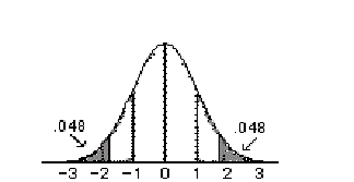
\(p(z \ge 1.667) = 0.048\) and \(p(z \le -1.667) = 0.048\)
so \(p-value = 0.096\) or 9.6%
- Make a decision: reject or fail to reject the null hypothesis
The p-value is the probability of observing a z-statistics as extreme as the one observed, given the null hypothesis. If the probability is “too small” (i.e, under the null hypothesis, it is highly unlikely to obtain the calculated z-statistics) we reject the null hypothesis. Otherwise, we fail to reject the null hypothesis. What does “too small” mean? We often compare the p-value to a stated significance level \(\alpha\). We reject if \(p-value \le \alpha\). It is a common practice to choose .1, .05, .01 for the value of \(\alpha\).
Aside: Some researchers say that a hypothesis test can have one of two outcomes: you accept the null hypothesis or you reject the null hypothesis. Many statisticians, however, take issue with the notion of “accepting the null hypothesis.” Instead, they say: you reject the null hypothesis or you fail to reject the null hypothesis. This is a philosophical argument that we will not get into. It suffices to know that both sides have a point. I recommend you use “fail to reject”. Read more: http://statistics.about.com/od/Inferential-Statistics/a/Why-Say-Fail-To-Reject.htm
Sources: http://stattrek.com/hypothesis-test/hypothesis-testing.aspx http://www.unc.edu/~jamisonm/fivesteps.htm
7.3 Comparing two means
We have covered how to statistically compare a population mean to a hypothetical value. Now, let’s look at how we can compare two populations’ means. Comparing two populations’ means follows the same principles as before, except that we need to do some fixes for the standard error. By definition, the standard error of the difference between two means is:
\[s_{x,y} = \sqrt{\frac{s^2_{\bar x}}{n_x}+\frac{s^2_{\bar y}}{n_y}}\]
Where:
\(s^2_{\bar x}\) is the variance for the sample x (male group for example)
\(s^2_{\bar y}\) is the variance for the sample y (female group for example)
\(n_x\) and \(n_y\) are respectively the number of observations in sample x and y.
The z-statistics equivalent for comparing two means is given by:
\[z^* = \frac{\bar X - \bar Y}{\sqrt{\frac{s^2_{\bar x}}{n_x}+\frac{s^2_{\bar y}}{n_y}}}\]
Once we have the calculated z-statistics (\(z^*\)), the decision rules covered above (section IV) applies. Moreover, the confidence interval procedure, covered before, applies to the means difference. The confidence interval for the difference between \(\mu_x\) and \(\mu_y\) (\(\mu_x - \mu_y\)) is given by:
\[CI = \Bigg[(\bar X - \bar Y) \pm z_{\alpha/2}\sqrt{\frac{s^2_{\bar x}}{n_x}+\frac{s^2_{\bar y}}{n_y}}\Bigg]\]
7.4 Decision Rule:
The analysis plan includes decision rules for rejecting the null hypothesis. In practice, statisticians describe these decision rules in two ways - with reference to a P-value or with reference to a region of rejection.
The P-value approach: the null hypothesis is rejected when the p-value is less than a predefined significance level (\(\alpha\)).
Rejection region approach: the null hypothesis is rejected when the calculated z-statistics is located in the rejection region, defined by the chosen significance level (\(\alpha\)).
Note: The two approaches are equivalent. Why?
7.5 Decision Errors: Types of errors
Two types of errors can result from a hypothesis test.
Type I Error: A Type I error occurs when we reject a null hypothesis when it is true. The probability of committing a Type I error is called the significance level (often noted as \(\alpha\)).
Type II Error: A type II error occurs when we fail to reject (i.e accept) the null hypothesis when we should reject it.
7.6 Two-Tailed Tests vs One-Tailed Test
The type of test we introduced in the first part of the lecture is often referred as a two tailed test (or two sided test). The test is set as follows: \[H_0: \mu = \mu_0\] \[vs.\] \[H_a: \mu \ not = \mu_0\]
In this case, we use:
\[|z^*| = |\frac{\bar X - \mu(hypothesized)}{s/\sqrt n}|\]
and compute our p-value as follows:
\[p-value = p(|z| \ge |z^*|)\]
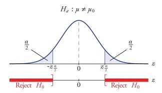
The shaded areas are called the rejection region. The null hypothesis is rejected when the calculated z-statistics \(z^*\) is in that region. The null hypothesis cannot be rejected when our calculated z-statistics is not located in that area.
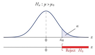
A test of a statistical hypothesis, where the region of rejection is on only one side of the sampling distribution, is called a one-tailed test. For example, suppose the null hypothesis states that the mean is less than or equal to 10. The alternative hypothesis would be that the mean is greater than 10. The region of rejection would consist of a range of numbers located on the right side of the sampling distribution; that is, a set of numbers greater than 10. The test can be stated as follows:
\[H_0: \mu \le \mu_0\] \[vs.\] \[H_a: \mu \gt \mu_0\] where \(\mu_0 = 10\) for our example.
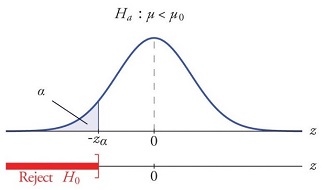
Of course, there are test that can be set as follow: \[H_0: \mu \ge \mu_0\] \[vs.\] \[H_a: \mu \lt \mu_0\]
In that case, the rejection region is as shown below.