6 Foundations for inference

In statistics, we are often interested in knowing some summary statistics about the population of interest (for example, the average income of all American adults, the median weight of all Nebraskans, the number of homeless people in Nebraska, …). It is very difficult to collect information on all American adults, or on all Nebraskans, or on all homeless people in Nebraska. In general, it is not practical to collect information on the whole population. So, we often rely on samples. But, how likely the summary statistics we get from a sample is representative of the summary statistics of the whole population. That is the subject of inferential statistics. Inferential statistics consists of generalizing from a sample to a population.

6.1 Variability in estimates (Sampling and Sampling Distribution)

Notice that if we take several samples from a population, each sample is likely to give us different summary statistics. Now, how can we generalize our findings if we have only a single sample of data? We will rely on the central limit theorem to make this generalization.

6.1.1 The Central Limit Theorem (CLT)

Basically, the CLT says that the sample mean $\bar X$ has a normal distribution with mean $\mu_{\bar X} = \mu$ and variance $\sigma^2_{\bar X} = \sigma^2/n$ . That is, the mean of $\bar X$ ( $\mu_{\bar X}$ ) is the same as the mean of the population ( $\mu$ ), and the variance of $\bar X$ ( $\sigma^2_{\bar X}$ ) is the variance of the population divided by the sample size n. Moreover, $\bar X$ has a bell curved type of distribution. What can we do with this information? ( hint: Think about the z-score)

Definitions:

$\mu$ and $\sigma^2$ refer to the population mean and variance respectively. They are called population parameters. By definition, a parameter is a numerical summary of the population.
$\bar X$ and $s^2$ refer to the sample mean and variance respectively. They are called sample statistics. By definition, a statistic is a numerical summary of a sample taken from the population.
The probability distribution of a statistic is called the “sampling distribution”.

Why do we need to know the CLT?
Answer: it provides the theoretical foundation of inferential statistics. By inferential statistics we mean generalizing from a sample to the general population.

Challenge: We are asked to think as if. Generally we only have one sample, so we have one mean. How then can we talk about sampling distribution of the mean? Note that our sample is just one sample. If we could get a new sample, that sample will likely be different. Assume we have the luxury of taking hundreds of samples with the same size n; then compute the mean for each sample. The set of computed means has a distribution. The central limit theorem tells us that if the sample size is big enough, this distribution is normal. What do we mean by big enough? There is no formal answer. Textbooks recommend that n=30 is good enough.
Can you see why we spent some time on the normal distribution?

Examples:
Find the mean and the standard deviation of the sampling distribution. You take a simple random sample (SRS) of size 25 from a population with mean 200 and standard deviation 10. Find the mean and standard deviation of the sampling distribution of your sample mean.

The effect of increasing the sample size. In the setting of the previous exercise, repeat the calculations for a sample size of 100. Explain the effect of the increase on the sample mean and standard deviation.

Note: We call the standard deviation of a statistic, standard error.

6.2 Confidence intervals

Recall, from previous lectures, that if the random variable $X$ follow a normal distribution with mean $\mu_{\bar X}$ and standard deviation $\sigma_{\bar X}$ , then we can convert the random variable $X$ to its standard form, i.e. $z_x = \frac{X-\mu_x}{\sigma_x}$

One reason we want to convert our data to standard form is that we can easily read off probabilities of some conditions on z-scores from the standard normal table (or the standard normal app) (see link http://www.mathsisfun.com/data/standard-normal-distribution.html). The picture below shows an example of a normaly distributed data and the standardized form of the same data. Remember that with the standardized form of the data, we can say something about the probabilities of some conditions on the z-scores. For example, what is the probability of $z \le -1$ ?

Standardized normal distribution

Example: Assume the random variable X follows a normal distribution with mean $\mu_{X} = 10$ and standard deviation $\sigma_X = 3$ . What is the probability that $X \ge 16$ ?

What is the probability that $4 \le X \le 16$ ?

Actually, we used 2 for simplicity when we said that about 95% of all observations fall within 2 standard deviations. Note that $P(-2 \le z \le 2) \not= 95\%$ (check that with the online app on normal distribution). $P(-2 \le z \le 2) = 95.4\%$ . We should use 1.96 instead of 2 if we want to get 95%, precisely (i.e $P(-1.96 \le z \le 1.96) = 95\%$ )

Recall also, from section 5.1.1, that the CLT says that the sample mean ( $\bar X$ ) has a normal distribution with mean $\mu_{\bar X} = \mu$ and variance $\sigma^2_{\bar X} = \sigma^2/n$ . $\mu$ is the population mean (also called true mean), and $\sigma^2$ is the population variance (also called true variance).

The z-score for any $\bar X$ is then: $z_{\bar X} = \frac{\bar X - \mu_{\bar X}}{\sigma_{\bar X}} = \frac{\bar X - \mu}{\sigma/\sqrt n}$

Based on 1 and 2, we know that:

$P(-1.96 \le z_{\bar X} \le 1.96) = 95\%$ . We can derive the formula of confidence interval as:

$P(-1.96 \le \frac{\bar X - \mu_{\bar X}}{\sigma_{\bar X}} \le 1.96) = 95\% \Longleftrightarrow$

$P(-1.96 \le \frac{\bar X - \mu}{\sigma/\sqrt n} \le 1.96) = 95\% \Longleftrightarrow$

$P(-1.96\sigma/\sqrt n \le \bar X - \mu\le 1.96\sigma/\sqrt n) = 95\% \Longleftrightarrow$

$P(-1.96\sigma/\sqrt n - \bar X \le - \mu\le 1.96\sigma/\sqrt n - \bar X) = 95\% \Longleftrightarrow$

$P(1.96\sigma/\sqrt n + \bar X \ge \mu\ge - 1.96\sigma/\sqrt n + \bar X) = 95\% \Longleftrightarrow$

$P(\bar X - 1.96\sigma/\sqrt n \le \mu\le \bar X + 1.96\sigma/\sqrt n) = 95\%$

The interval $[\bar X - 1.96 \sigma / \sqrt n \ , \ \bar X + 1.96 \sigma/\sqrt n ]$ is known as the 95% confidence interval, or the 95% interval estimate. The following picture illustrates the idea of confidence interval:

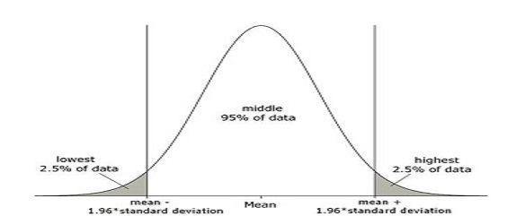
Idea of confidence interval

Note: 1.96 is the value of z that gives us 95% confidence interval. It is noted $z_{0.025}$ because we have 2.5% of observations that lie above that z. More generally, we will write $z_{\alpha}$ to refer to the value of z for which the proportion of observations lying above it is $\alpha/2$ . Thus, the general formula of the confidence interval is: $[\bar X - z_{\alpha/2}\sigma/\sqrt n \ , \ \bar X + z_{\alpha/2}\sigma / \sqrt n]$

Most of the time, we will be using $\alpha = 1%$ , $\alpha = 5%$ , or $\alpha = 10%$ . Why these number? It is just a tradition.

Level of Confidence

Problem: How would you interpret the interval $[\bar X - z_{\alpha/2}\sigma/\sqrt n \ , \ \bar X + z_{\alpha/2}\sigma / \sqrt n]$ .

Wouldn’t we get a different interval if we had a different sample? The answer is yes! Then, what does our interpretation really mean?

Every sample will likely give us a different interval, and they cannot all mean what our naïve interpretation says.

Here is the interpretation of confidence interval: A proportion of $(1-\alpha)$ of such intervals will contain the true value of the parameter (the mean $\mu$ in our case). This is a little bit technical.

Here is another interpretation: We are $(1-\alpha)100\%$ confident that the interval $[\bar X - z_{\alpha/2}\sigma/\sqrt n \ , \ \bar X + z_{\alpha/2}\sigma / \sqrt n]$ includes the population mean.

$z_{\alpha/2}\sigma/\sqrt n$ is refers as the margin of error; and $(1-\alpha)$ is refers as the confidence level.

Practice Question:

Discount Sounds has 260 retail outlets throughout the United States. The firm is evaluating a potential location for a new outlet, based in part, on the mean annual income of the individuals in the marketing area of the new location.

A sample of size n = 36 was taken; the sample mean income is $41,100. The population standard deviation is estimated to be $4,500, and the confidence coefficient to be used in the interval estimate is 0.95.

What is the margin of error?
What is the confidence interval for the population mean?
Interpret the confidence interval.

Values of $z_{\alpha/2}$ for the Most Commonly Used Confidence Levels are:

Confidence Level	$\alpha$	$\alpha/2$	$z_{\alpha/2}$
90%	10	5	1.645
95%	5	2.5	1.96
99%	1	0.5	2.576