Chapter 2 TURF
TURF analysis (Total Unduplicated Reach and Frequency analysis) is a market research technique that helps companies identify the optimal product or service offering for a target market by analyzing the total reach and frequency of different combinations of offerings. TURF analysis is particularly useful when a company has a range of products or services and wants to know which combination will maximize its market penetration. By analyzing the unduplicated reach (the number of unique customers reached) and frequency (the number of times customers are reached) of different product or service combinations, companies can determine which offerings are most likely to appeal to the largest number of customers. TURF analysis involves creating a matrix of all possible product or service combinations, then calculating the unduplicated reach and frequency for each combination. The results are then analyzed to determine which combination or set of offerings will provide the highest total reach and frequency.
Let’s make an example: suppose we have a collection of k items, and we want to determine the set of items that has the highest reach. We can start by collecting data on consumer choices across the items and hot-encoding them (1 if respondent i selected item k and 0 otherwise). This results in a dataset with k columns (each column is an item) and n rows (equal to the number of respondents). (Let’s deal with the frequency of purchase later).
If the set is made of only one item or all items, the choice is straightforward. We choose the item with the highest reach in the first scenario, while we choose all items in the latter. However, for bundle sizes greater than 2 and less than the maximum size, the process becomes more complicated.
For \(k\geq2\) we have N possible combinations of item, where N is given by the binomial coefficient: \(N=\binom{n}{k}=\frac{n!}{k!(n-k)!}\). It gives us how many unique different ways there are to choose k items from n items set.
For example, if k=2 and n=10 there are N=45 combinations, listed below
| Item | 1 | 1 | 1 | 1 | 1 | 1 | 1 | 1 | 1 | 2 | 2 | 2 | 2 | 2 | 2 |
| Item | 2 | 3 | 4 | 5 | 6 | 7 | 8 | 9 | 10 | 3 | 4 | 5 | 6 | 7 | 8 |
| Item | 2 | 2 | 3 | 3 | 3 | 3 | 3 | 3 | 3 | 4 | 4 | 4 | 4 | 4 | 4 | 5 |
| Item | 9 | 10 | 4 | 5 | 6 | 7 | 8 | 9 | 10 | 5 | 6 | 7 | 8 | 9 | 10 | 6 |
| Item | 5 | 5 | 5 | 5 | 6 | 6 | 6 | 6 | 7 | 7 | 7 | 8 | 8 | 9 |
| Item | 7 | 8 | 9 | 10 | 7 | 8 | 9 | 10 | 8 | 9 | 10 | 9 | 10 | 10 |
Once we have all the possible combinations of items of size 2, we can loop over these combinations and record for each individual whether he/she selected at least one of the items in the combination or not. We set the record variable to 1 if the individual has chosen at least one item from the selected combination and 0 otherwise. To determine the reach of each combination, we divide the sum of the records of each combination by the size of the sample. If we take into account the frequency of purchase, the computation is slightly different as we should weight each individual by its purchasing frequency. In other words, it is a simple average when we do not consider frequency, while it is a weighted average when we do consider frequency. For instance in the case of k = 2 and n=10, the first combination is made of \(x_{1}\) and \(x_{2}\) therefore the record variable (let’s call it \(R(x_{1}, x_{2})\)) is created as follows: \[ R(x_{1}, x_{2})= \begin{cases} 1 & \text{if}\ \text{respondent chooses } \{x_{1}\cup{x_{2}}\} \\ 0 & \text{otherwise} \end{cases} \] The reach is calculated as: \(Reach(x_{1}, x_{2})=\frac{\sum_{i=1}^{n} R(x_{1}, x_{2})}{n}\), where n is the sample size. We then proceed in calculating the reach for all two-combinations of items. (If we consider the frequency of purchase we should compute a weighted average: \(Reach(x_{1}, x_{2})=\frac{\sum_{i=1}^{n} w(R(x_{1}, x_{2}))}{\sum_{i=1}^{n} w}\) where \(w\) are the weights).
# Load data
dir <- "C:\\Users\\roal2007\\Desktop\\learning\\TURF\\"
load(file = paste0(dir, "turf_ex_data.rda"))
dt <- turf_ex_data[stringr::str_detect(colnames(turf_ex_data), "item")==T]
## number of items
N = ncol(dt)
## names of items
item_list = colnames(dt)
c=2
#### possible combinations of c
combinations <- combn(ncol(dt), c)
## loop thorugh each column (variable)
reach_comb <- apply(combinations, 2, function(cols) {
  ### record variable, equal to 1 if at least one of the items in the selected combination is selected (ie the sum of the columns selected is > 0)
  record <- rowSums(dt[,cols] == 1) > 0
  ## calculate the mean (ie the reach)
  reach <- mean(record)
  ### extract the names of the items
  item_name <- paste0(names(dt)[cols], collapse = ";")
  c(item_name, reach)
})
### transpose the matrix
reach_comb <- t(reach_comb)
reach_comb <- data.frame(item = reach_comb[,1], share = as.numeric(reach_comb[,2]))
### multiply *100 to have percentages
reach_comb <- reach_comb %>%
  mutate(share = round(share*100,2))

turf_res <- reach_comb
## V1 V2 V3 V4 V5 V6 V7 V8 V9 V10 V11 V12 V13 V14 V15
## Item 1 1 1 1 1 1 1 1 1 2 2 2 2 2 2
## Item 2 3 4 5 6 7 8 9 10 3 4 5 6 7 8
## Reach 25.56 40.56 42.22 52.78 67.78 73.33 78.33 82.22 91.11 47.78 49.44 57.22 70.56 74.44 77.22
## V16 V17 V18 V19 V20 V21 V22 V23 V24 V25 V26 V27 V28 V29 V30
## Item 2 2 3 3 3 3 3 3 3 4 4 4 4 4 4
## Item 9 10 4 5 6 7 8 9 10 5 6 7 8 9 10
## Reach 83.89 92.22 62.78 67.78 73.33 78.89 82.78 86.67 91.67 68.33 78.89 82.22 83.89 87.22 94.44
## V31 V32 V33 V34 V35 V36 V37 V38 V39 V40 V41 V42 V43 V44 V45
## Item 5 5 5 5 5 6 6 6 6 7 7 7 8 8 9
## Item 6 7 8 9 10 7 8 9 10 8 9 10 9 10 10
## Reach 80 82.78 85 89.44 93.89 89.44 90 92.22 93.89 93.89 94.44 96.67 95 96.67 98.33We can perform this process for all possible sets ranging from size 1 up to the maximum size of 10 in this example. We then determine the combination with the highest reach for each set size to identify the optimal set. The resulting output is displayed in the following plot.
## Let's write a function so that we can compute the reach for any combination c
turf <- function(dt, c) {

  # possible combinations of c
  combinations <- combn(ncol(dt), c)

  # loop through each column (variable)
  reach_comb <- apply(combinations, 2, function(cols) {

    # record variable, equal to 1 if at least one of the items in the selected combination is selected (ie the sum of the columns selected is > 0)
    ## for the case c=1 we need to adjust the code a little
    if (c > 1) {
      record <- rowSums(dt[, cols] == 1) > 0
    } else {
      record <- as.numeric(dt[, cols])
    }

    # calculate the mean (ie the reach)
    reach <- mean(record)

    # extract the names of the items
    item_name <- paste0(names(dt)[cols], collapse = ";")

    c(item_name, reach)
  })

  # transpose the matrix
  reach_comb <- t(reach_comb)

  # convert to data frame, rename columns, and format percentages
  reach_comb <- as.data.frame(reach_comb, stringsAsFactors = FALSE)
  colnames(reach_comb) <- c("item", "share")
  reach_comb$share <- as.numeric(reach_comb$share) * 100
  ### arrange(desc()) sort results in desceding order on variable share
  reach_comb <- reach_comb %>% arrange(desc(share))

  return(reach_comb)
}

## let's call the function for all possible combinations and store the results in a list
res_all <- list()
for(i in 1:N){
  res_temp <- turf(dt, i)
  res_temp. <- list(res_temp)
  res_all <- append(res_all, res_temp., after = (i-1))
}

## extract max reach for each number of combinations
max_reach <- cbind(1:N,sapply(res_all, function(x) {
  max_r <- round(max(x[, 2]),2)
  c(max_r)
}))

max_reach <- as.data.frame(max_reach)
colnames(max_reach) <- c("N", "Reach")

ggplot(max_reach, aes(x = N, y = Reach)) +
  geom_point(size = 3) +
  geom_line() + scale_x_continuous(breaks=c(1:10))+
  labs(title = "", x = "N", y = "Reach")+theme_classic()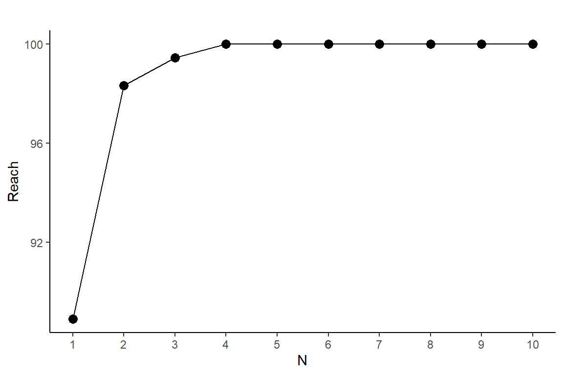
For this example, a set containing 4 items achieves the maximum reach, but a set with 2 items is also considered a satisfactory result. (It’s important to consider the incremental change at each step when evaluating the optimal set.) We select the set with 2 items as the optimal one, and then extract the combinations of items with the highest reach. The table below displays the first 10 combinations.
k = 2
datplot <- turf(dt, k)
datplot <- as.data.frame(datplot)
## subset first 10 combinations made of c items
datplot <- datplot[1:10,]| best_items | reach |
|---|---|
| item_9 item_10 | 98.33% |
| item_7 item_10 | 96.67% |
| item_8 item_10 | 96.67% |
| item_8 item_9 | 95% |
| item_4 item_10 | 94.44% |
| item_7 item_9 | 94.44% |
| item_5 item_10 | 93.89% |
| item_6 item_10 | 93.89% |
| item_7 item_8 | 93.89% |
| item_2 item_10 | 92.22% |
The differences between the best combinations appear to be so small that it’s unclear whether they are statistically significant or just due to chance. To test for statistical significance, we can estimate the standard errors using a technique called bootstrap. (A detailed section on bootstrap is coming.)
Bootstrap is a resampling method used to estimate the standard errors and confidence intervals of a statistical estimate, such as a mean or a regression coefficient. The procedure involves repeatedly sampling observations from the original data set with replacement, creating many new “bootstrap samples” of the same size as the original data set. For each bootstrap sample, the same statistic is computed as in the original data set. By doing this process many times (usually N=1000), we get a distribution of the statistic across the different bootstrap samples. This distribution represents the sampling variability of the statistic, which can be used to estimate its standard error. The standard error of the estimate is then calculated from the standard deviation of the distribution of the statistic across the bootstrap samples. Confidence intervals for the estimate can also be calculated using this distribution.