Chapter 6 Dimensionality Reduction

Principal Component Analysis (PCA) is a statistical technique used for reducing the dimensionality of a dataset while retaining as much information as possible. In simple terms, it involves transforming a set of correlated variables into a smaller set of uncorrelated variables, called principal components. The first principal component accounts for the most variance in the data, followed by the second component, and so on, with the condition that each component is independent (uncorrelated to) from the others.

Here’s a step-by-step overview of how PCA works:

Standardize the data: PCA works best when the variables are on the same scale, so the first step is often to standardize the data by subtracting the mean and dividing by the standard deviation.
Compute the covariance matrix: The covariance matrix describes the relationships between the variables in the dataset. It is computed by taking the dot product of the standardized data matrix and its transpose.
Compute the eigenvectors and eigenvalues: The eigenvectors are the directions in which the data varies the most, and the eigenvalues are the amount of variance explained by each eigenvector. The eigenvectors and eigenvalues are computed from the covariance matrix.
Choose the number of principal components: We can choose to keep all of the principal components, or we can select a smaller subset based on how much variance we want to explain.
Transform the data: We can then transform the original data into the lower-dimensional space spanned by the principal components. Each observation in the original dataset can be expressed as a linear combination of the principal components. We reduce the dimensionality of data by projecting the data into these new principal components, they become the new “axis” of the system.
Interpret the results: We can interpret the results by looking at the loadings, which describe how much each original variable contributes to each principal component. We can also plot the data in the lower-dimensional space to look for patterns and clusters.

Let’s decompose each step: the covariance matrix stores the variance of each variable and the cross-variable covariances, so if we have a nXd matrix where n is given by the number of rows (individuals) and d the number of columns (variables), the covariance matrix is given by: \[ VARCOV=\boldsymbol{\Sigma}=\begin{Bmatrix} Var(X_{1}) & Cov(X_{1},X_{2}) & ... & Cov(X_{1},X_{d}) \\ Cov(X_{2},X_{1}) & Var(X_{2}) & ... & ... \\ ... & ... & ... & ...\\ Cov(X_{d},X_{1}) & ... & ... & Var(X_{d}) \end{Bmatrix} \]

The covariance matrix defines both the spread (variance) and the orientation (covariance) of our data (positively correlated variables tend to “move” together and conversely for negatively correlated variables). Let’s make an example to visualize it: \[ \boldsymbol{\Sigma}=\begin{Bmatrix} 7 & 0.2 \\ 0.2 & 2 \end{Bmatrix} \]

Is the covariance matrix of the following dataset:

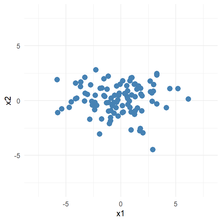
We can see that the data vary most on the x1 variable while little on the x2 variable.

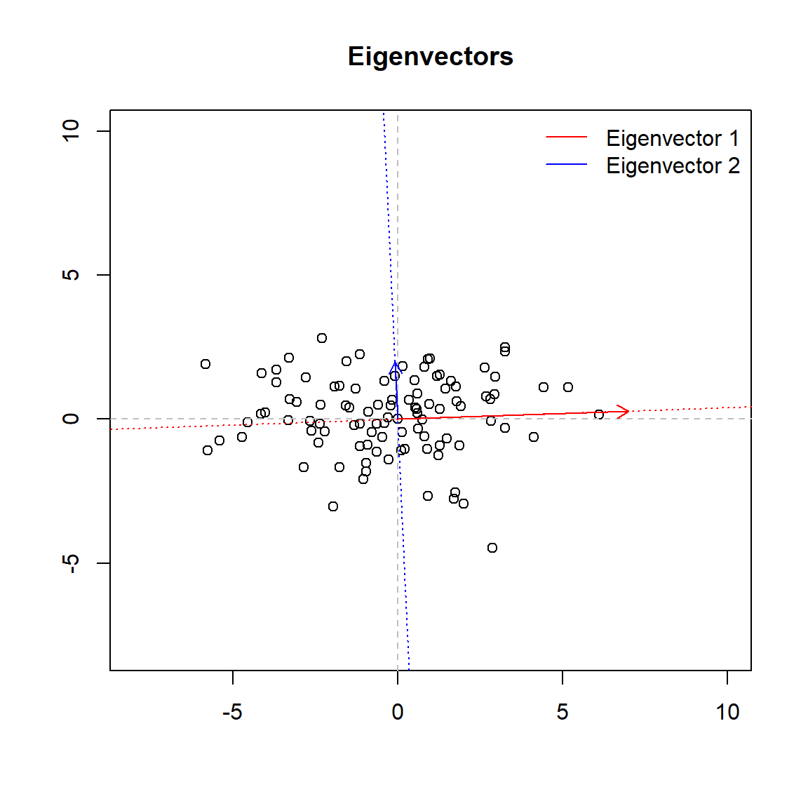
To this matrix can be assigned two further elements: a representative vector (the eigenvector) and a number which indicates its magnitude (the eigenvalue). The vector will point into the direction of the larger spread of data, the number will be equal to the spread (variance) of that direction.

\[\begin{equation} \boldsymbol{\Sigma} \boldsymbol{v}_i = \lambda_i \boldsymbol{v}_i \end{equation}\]

where \(\lambda_i\) is the \(i\)-th eigenvalue and \(\boldsymbol{v}_i\) is the corresponding eigenvector.

In simple terms, an eigenvector is a vector that, when multiplied by a matrix, is only scaled by a scalar value. This scalar value is called the eigenvalue. In other words, the eigenvector is a special vector that does not change its direction when it is transformed by the matrix, only its length is multiplied by the eigenvalue.

Below we plot the two eigenvectors (the lenght of the vector is proportional to the eigenvalue). You can think of egeinvectors as the directions in which the data varies the most. In this example the first eigenvector of the covariance matrix points in the direction of \(x_{1}\) axis, it means that the variability in the data is mostly along this variable (as can be easely seen from the graph and the covariance matrix). The second principal component is uncorrelated with (i.e., perpendicular to) the first principal component and accounts for the next highest variance (in this case for the remaining variance). So in this case once we know the first eigenvector we already know the second as its the vector perpendicular to the first one.

We then select the first \(k\) eigenvectors to form the projection matrix, in this example we select both eigenvectors. We project the original data matrix \(\boldsymbol{X}\) onto the projection matrix multiplying the two: \[\begin{equation} \boldsymbol{Z} = \boldsymbol{X} \boldsymbol{W} \end{equation}\] where \(\boldsymbol{Z}\) is the \(n \times k\) matrix of transformed data points. We call the columns of the new matrix scores, which are not other than the values obtained by projecting the data onto the new coordinate system defined by the principal components. The projection matrix \(\boldsymbol{W}\) contains the loadings of each original variable onto each principal component, which are not other than the values of the eigenvectors, which give us the weight of each variable into each component. \[ \boldsymbol{W}=\begin{Bmatrix} \boldsymbol{v}_1 & \boldsymbol{v}_2 \end{Bmatrix}=\begin{Bmatrix} \phi_{1,1} & \phi_{2,1} \\ \phi_{2,1} & \phi_{2,3} \end{Bmatrix} \] If we decide to keep both components than \(\boldsymbol{Z}\) will have two columns, corresponding to the score derived from each component \[ \begin{equation} Z_{1}=x_{1}\phi_{1,1}+x_{2}\phi_{2,1} \end{equation} \] \[ \begin{equation} Z_{2}=x_{1}\phi_{1,2}+x_{2}\phi_{2,2} \end{equation} \] PCA in this example is not be particularly useful, as you can easily plot the raw data on a scatter plot to visualize the relationship between the two variables. PCA is most useful when you have high-dimensional data, where it can help to identify patterns and relationships that are difficult to see in the original data space.

Let’s do an example with real data, we will use the USArrest dataset which collects statistics on violent crime rates in the United States. It includes data on the number of arrests per 100,000 residents for three different types of crimes (murder, rape and assault) and the urban population in each of the 50 states of the United States.

We start by standardizing the dataset, we subtract to each variable its mean and divide by its standard deviation, we obtain the new standardized dataset \(\mathbf{\tilde{X}}\). We then compute the covariance matrix and its corresponding eigenvectors and eigenvalues.

data(USArrests)

# Standardize the data
USArrests_scaled <- scale(USArrests)

# Compute the covariance matrix
cov_matrix <- cov(USArrests_scaled)

# Compute the eigenvectors and eigenvalues
eigen_values <- eigen(cov_matrix)$values
eigen_vectors <- eigen(cov_matrix)$vectors
rownames(eigen_vectors) <- names(USArrests)
colnames(eigen_vectors) <- c("PC1", "PC2", "PC3", "PC4")
print(eigen_vectors)

##                 PC1        PC2        PC3         PC4
## Murder   -0.5358995  0.4181809 -0.3412327  0.64922780
## Assault  -0.5831836  0.1879856 -0.2681484 -0.74340748
## UrbanPop -0.2781909 -0.8728062 -0.3780158  0.13387773
## Rape     -0.5434321 -0.1673186  0.8177779  0.08902432

print(eigen_values)

## [1] 2.4802416 0.9897652 0.3565632 0.1734301

Here are printed the 4 eigenvectors (in general there are \(m\) eigenvectors where \(m=min(n-1,d)\) with their corresponding eigenvalues, already sorted in descending orderd by the value of the eigenvalues (so that the first eigenvector is the one that accounts for most of the variance, the second is the vector that account for most of the variance, and so on; under the condition that all these new eigenvectors are independent (uncorrelated) among each other).

To choose the number of components we can calculate how much variance is explained by each component. Variance of the component is equal to the square of the corresponding eigenvalue.

Below is the proportion of variance explained by each component.

## [1] "62.01%" "24.74%" "8.91%"  "4.34%"

While here we show the cumulative proportion of explained variance by each component

## [1] "62.01%" "86.75%" "95.66%" "100%"

In this example the first two components account for more than 80% of the total variance. Before proceeding into transforming the original dataframe we want to know to what variables these two components refer to. These are given by the values in the eigenvectors, the first component is mostly correlated to murder, assualt and rape, while the second component to Urbanpop.

We then transform the data into two dimensions, multiplying the original scaled dataframe (\(\mathbf{\tilde{X}}\)) by the first two principal components. So that we will end up with two variables, called scores. \[\begin{equation} Score_{PC1}=\tilde{x_{1}}\phi_{PC1,x_{1}}+\tilde{x_{2}}\phi_{PC1,x_{2}}+\tilde{x_{3}}\phi_{PC1,x_{3}}+\tilde{x_{4}}\phi_{PC1,x_{4}} \end{equation}\] \[\begin{equation} Score_{PC2}=\tilde{x_{1}}\phi_{PC2,x_{1}}+\tilde{x_{2}}\phi_{PC2,x_{2}}+\tilde{x_{3}}\phi_{PC2,x_{3}}+\tilde{x_{4}}\phi_{PC2,x_{4}} \end{equation}\]

# Transform the data (ie. reduce to two dimension, the first two principal components)
transformed_data <- USArrests_scaled %*% eigen_vectors[,1:2]

To better visualize the output we can use special plot called biplot, which is a type of graphical display that allows to simultaneously display both the scores and the loadings of the variables in a two-dimensional plot. The scores are the coordinates of the observations in the new coordinate system defined by the principal components. The loadings represent the contribution of each variable to each principal component and are plotted on two different axis (top axis correspond to the weight of the variable in the first component; and left axis correspond to the weight the variable has in the second component) in the same plot.