Chapter 4 Clustering
4.1 K-means clustering
Clustering is a type of unsupervised machine learning technique used to group together similar data points based on their characteristics. The goal of clustering is to identify groups or clusters within a dataset that share common traits, patterns or features. The resulting clusters can then be used to gain insights into the data, make predictions, or take actions.
K-means clustering is a popular clustering algorithm that partitions a dataset into k clusters based on their distance to the cluster centroids (the vector containing the average of each dimension). The algorithm first randomly assigns each data point to a cluster, it then computes the centroid of each cluster k and assign each observation to the nearest centroid, based on a chosen distance metric such as Euclidean distance (it is the length of the straight line that connects two points in that space \(d=\sqrt{(x_{2}-x_{1})^{2}+(y_{2}-y_{1})^{2}}\), and can be easily extended to each number of dimension: \(d=\sqrt{(x_{2}-x_{1})^{2}+(y_{2}-y_{1})^{2}+(z_{2}-z_{1})^{2}+...}\)) (* There are many dissimilarities measure, the choice depends on the nature and distribution of the data, as well as the requirements of the clustering algorithm. For certain type of data a measure based on correlation may be better suited). The centroids are then updated to the mean of the data points in their respective clusters. The assignment and update steps are repeated until the clusters no longer change significantly or a maximum number of iterations is reached. The resulting clusters are optimized to minimize the sum of squared distances between the data points and their respective centroids.
Formally, the k-means algorithm can be described as follows:
- Randomly assign each observation to a cluster k and compute clusters centroids
- Assign each data point to the cluster whose centroid is nearest
- Recalculate the centroids of each cluster as the mean of the data points assigned to it.
- Repeat steps 2 and 3 until the cluster assignments no longer change or a maximum number of iterations is reached.
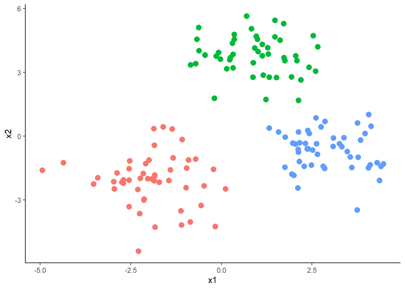
Let’s explain it with a fake dataset.
rm(list = ls())
set.seed(77)
cluster1 <- data.frame(x1 = rnorm(50, mean = 1, sd = 1)-3,
                       x2 = rnorm(50, mean = 1, sd = 1)-3,
                       cluster = "A")
cluster2 <- data.frame(x1 = rnorm(50, mean = 1, sd = 1),
                       x2 = rnorm(50, mean = 1, sd = 1)+3,
                       cluster = "B")
cluster3 <- data.frame(x1 = rnorm(50, mean = 1, sd = 1)+2,
                       x2 = rnorm(50, mean = 1, sd = 1)-2,
                       cluster = "C")

# Combine the two clusters into a single dataset
ogdata <- as.data.frame(rbind(cluster1, cluster2, cluster3))
This code creates three clusters of data, each with 50 observations and two variables (\(x_{1}\) and \(x_{2}\)). Each cluster is generated by randomly sampling 50 observations from a normal distribution with a different mean and standard deviation.
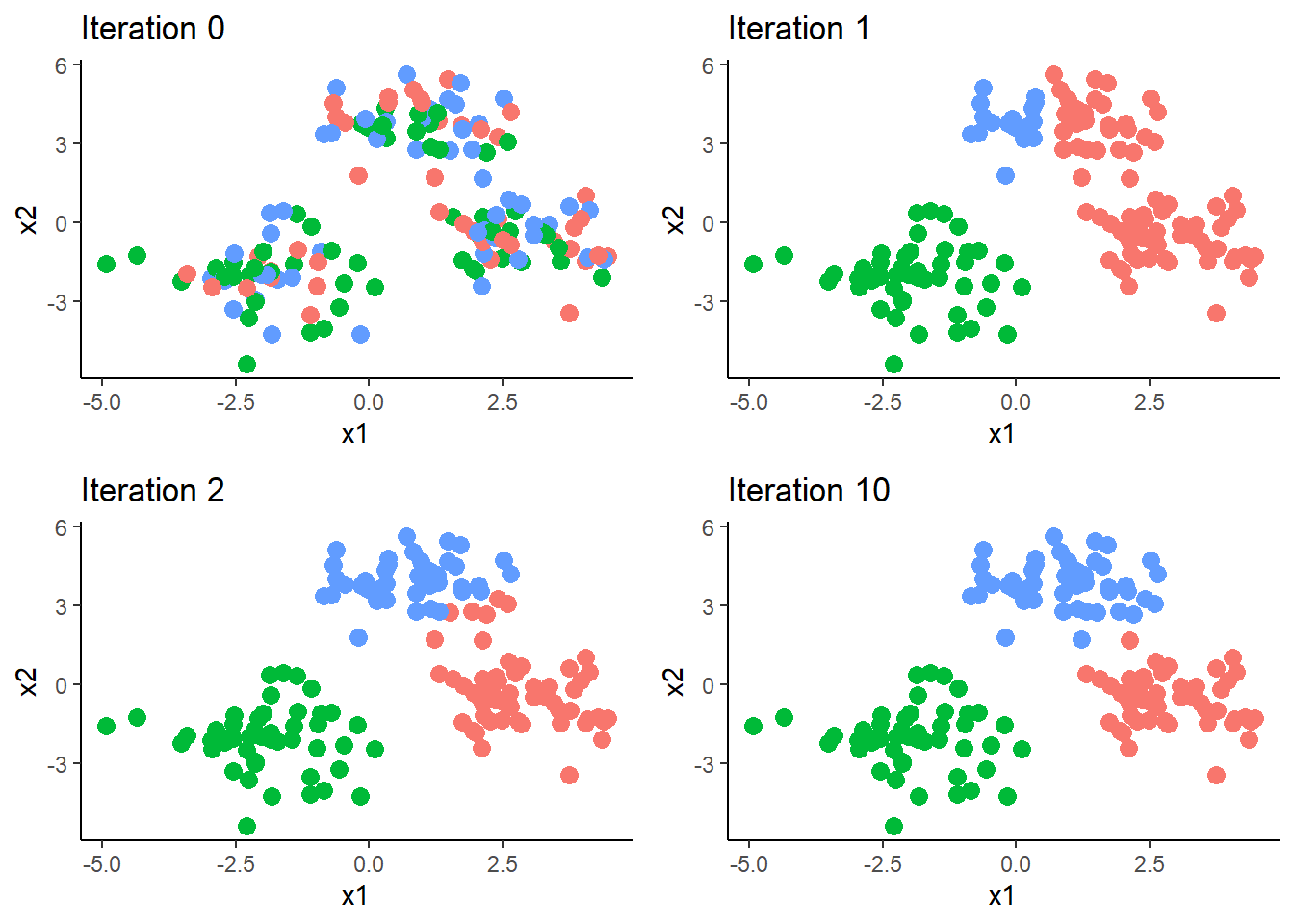
We start the process by selecting how many clusters we want to group the data into, and random assign each observations to 1 of the k clusters. We know that the data have three “natural” clusters and therefore choose k to be 3. After assiging the observations we compute the centroid for each cluster. \[ \begin{equation} \mu_{k}={\boldsymbol{\bar{X}}_{i\in{C_{k}}}}=\begin{Bmatrix} \frac{1}{n_{k}}\sum_{i\in{C_{k}}}^{n_{k}}x_{1} & \frac{1}{n_{k}}\sum_{i\in{C_{k}}}^{n_{k}}x_{2}\end{Bmatrix} \end{equation} \] Where \(n_{k}\) is the number of observations in cluster k. We then compute the distance between observation i and each of the k clusters. For each observation i we calculate:
\[\begin{equation} \boldsymbol{d_{i}}=\begin{Bmatrix} \sqrt{(\boldsymbol{x_{i}-\mu_{k_{1}}})^{2}} & \sqrt{(\boldsymbol{x_{i}-\mu_{k_{2}}})^{2}} & \sqrt{(\boldsymbol{x_{i}-\mu_{k_{3}}})^{2}} \end{Bmatrix} \end{equation} \]
And reassign it to nearest cluster, the cluster for \(\boldsymbol{d_{i}}\) is the minimum. We then repeat this process until the cluster assignments no longer change.
data <- ogdata[,1:2]

## number of clusters
k=3

## 1 step: random assign obs to clusters
y <- sample(1:k, nrow(data),replace = T)
yo <- y
Y <- matrix(data = NA, nrow = nrow(data), ncol = 10)
for(t in 1:10){
  # Compute cluster centroids for each cluster
  centroids <- matrix(0, nrow=k, ncol=ncol(data))
  for(i in 1:k){
    centroids[i,] <- colMeans(data[y==i,])
  }

  # Assign observations to nearest cluster
  dists <- apply(data, 1, function(x) sqrt(rowSums((x - centroids)^2)))
  y_new <- apply(dists, 2, which.min)

  y <- y_new
  Y[,t] <- y

}

data$group <- y
Please note this is just a toy example, in most practical applications data are scaled before running the clustering algorithms. K-means clustering is a distance-based clustering technique and thus is sensitive to the scale of the data, meaning that if the features of the data are measured in different units or have different scales, the clustering results may be biased towards the features with higher variances or larger scales. By scaling the data, we ensure that each feature is measured on the same scale and has equal importance in the clustering process. Usually data are normalized to have mean 0 and standard deviation of 1. A further detail to note is that the final clusters depend on the initial random assignments of the data points, therefore in most practical applications the algorithm is run N times, each time with a different initial random assignment and the best solution is selected. Here the best solution is the one that minimizes average within cluster variation. We can calculate the within cluster variation for each cluster k computing all the pairwise squared euclidean distances within the cluster and calculate the average, we then compute the average of all the within cluster variation. Formally, for each cluster k we compute the average within cluster variation: \[ \begin{equation} \frac{1}{n_{k}}\sum_{i\in{C_{k}}}^{n_{k}}(\mathbf{x_{i}}-\mathbf{\bar{x}_{i\in{C_{k}}}})^2 \end{equation}\]
The above algorithm minimizes the average of the k within cluster variations.
### within variation of each cluster
data %>% group_by(group) %>%
  mutate(within_variation=(x1-mean(x1))^2+(x2-mean(x2))^2) %>%
  summarise(avg_within_var = mean(within_variation))
## # A tibble: 3 × 2
## group avg_within_var
## <int> <dbl>
## 1 1 1.62
## 2 2 2.42
## 3 3 1.63## average within variation
data %>% group_by(group) %>%
mutate(within_variation=(x1-mean(x1))^2+(x2-mean(x2))^2) %>%
ungroup() %>% summarise(avg_within_var = mean(within_variation))## # A tibble: 1 × 1
## avg_within_var
## <dbl>
## 1 1.894.2 Hierarchical clustering
In K-means clustering, the number of clusters needs to be pre-specified, which can be challenging since it is not always clear how many clusters the data should be divided into. To overcome this limitation we can use as alternative hierarchical clustering, which creates a hierarchical structure of nested clusters, starting with all data points as individual clusters and then merging them iteratively based on their similarity. The result is a dendrogram that shows how the clusters are merged at different levels of similarity.
One of the main advantages of hierarchical clustering is that it allows us to explore different levels of clustering without having to commit to a specific number of clusters. By cutting the dendrogram at different heights, we can obtain different numbers of clusters, which provides a more nuanced understanding of the structure of the data. This flexibility makes hierarchical clustering a popular choice for exploratory data analysis and visualization.
To start hierarchical clustering, we first need to define how different or similar each observation is to each other. Euclidean distance is often used as the measure of similarity, but we can choose other measures as well.
The algorithm then proceeds in a step-by-step manner. At the beginning, each observation is treated as its own cluster. Next, we find the two most similar clusters and merge them into one cluster, reducing the total number of clusters by one. We repeat this process, merging the two most similar clusters at each step, until there is only one cluster left. When we merge two clusters, we need to define how dissimilar they are to each other. This is done using the concept of linkage, which extends the notion of dissimilarity from individual observations to groups of observations.
There are several types of linkage methods commonly used. The complete linkage method defines the dissimilarity between two clusters as the maximum distance between any two points in the two clusters. The single linkage method, on the other hand, uses the minimum distance between any two points in the two clusters. The average linkage method takes the average distance between all pairs of points in the two clusters.
By using different linkage methods, we can obtain different clustering results, so it’s important to choose the linkage method that best fits the data and problem at hand.
Let’s apply it to the above dataset.
set.seed(77)
cluster1 <- data.frame(x1 = rnorm(15, mean = 1, sd = 1)-3,
                       x2 = rnorm(15, mean = 1, sd = 1)-3)
cluster2 <- data.frame(x1 = rnorm(15, mean = 1, sd = 1),
                       x2 = rnorm(15, mean = 1, sd = 1)+3)
cluster3 <- data.frame(x1 = rnorm(15, mean = 1, sd = 1)+2,
                       x2 = rnorm(15, mean = 1, sd = 1)-2)

# Combine the two clusters into a single dataset
data <- as.data.frame(rbind(cluster1, cluster2, cluster3))


hc.complete <- hclust(dist(data), method = "complete")
hc.average <- hclust(dist(data), method = "average")
hc.single <- hclust(dist(data), method = "single")
###
par(mfrow = c(1, 3))
plot(hc.complete, main = "Complete Linkage",
     xlab = "", sub = "", cex = .9)
plot(hc.average, main = "Average Linkage",
     xlab = "", sub = "", cex = .9)
plot(hc.single, main = "Single Linkage",
     xlab = "", sub = "", cex = .9)
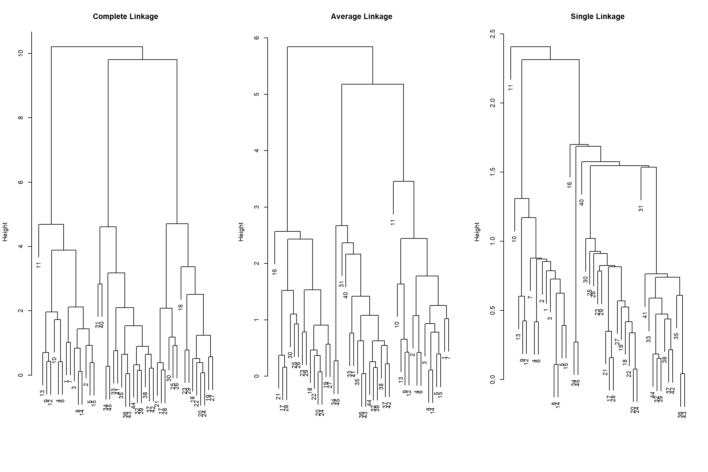
We can see from the graphs that, average and complete linkage tend to yield more balanced dendrograms, and are thus generally preferred over single linkage.
In this example, observations 9 and 12 are merged pretty soon. The height of the dendogram, that represents the distance between the two clusters at which they become a single cluster is pretty small. We can compute it as follows (note that for single observations the dissimilarity measure is the same for each linkage method as groups of observations are not involved).
pairwise_dist <- function(data) {
  n <- nrow(data)
  distances <- matrix(0, n, n)
  for (i in 1:(n-1)) {
    for (j in (i+1):n) {
      distances[i, j] <- sqrt(sum((data[i,] - data[j,])^2))
      distances[j, i] <- distances[i, j]
    }
  }
  return(distances)
}

dist_mat <- pairwise_dist(data)
cat("Distance between observation 9 and 12:", round(dist_mat[9,12],2))
## Distance between observation 9 and 12: 0.42While the dissimilarity among clusters, assuming complete linkage, is:
## Distance between cluster 2 and 3: 10.21## Distance between cluster 1 and 3: 9.82## Distance between cluster 2 and 3: 9.81We can see that cluster 2 and 3 are the most similar to each other among the remaining clusters and therefore are fused together; after it, cluster 2, the last cluster is finally added.
To determine the number of clusters one common method is to cut the dendrogram at a certain height that corresponds to a meaningful level of similarity or dissimilarity. However, there is no definitive answer as to what height is appropriate, and the choice often depends on the context of the problem.
One approach is to visually inspect the dendrogram and identify any noticeable gaps or branches that can be interpreted as distinct clusters. Another approach is to use a quantitative method, such as the elbow method, to identify an optimal number of clusters based on a measure of cluster quality or compactness.
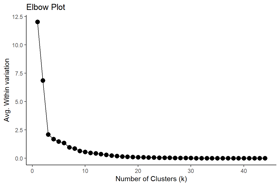
The elbow method involves plotting the average within-cluster sum of squares as a function of the number of clusters and selecting the number of clusters where the rate of decrease starts to level off, forming an “elbow” in the plot. It was easily predictable, the curve starts to level off once we have reached three clusters.
