Chapter 5 Conjoint

Conjoint analysis is a statistical technique used in market research to understand how people make trade-offs between different attributes of a product or service. It is a widely used method for estimating consumer preferences and determining the relative importance of different features of a product or service.

The basic idea behind conjoint analysis is to present respondents with a series of hypothetical product or service profiles, each varying in their combination of attributes, and ask them to rate or rank their preferences for each profile. By analyzing the patterns of responses across different profiles, we can estimate the relative importance of each attribute and its level or level combination that drives consumer preference.

For example, if we were interested in understanding consumers’ preferences for a new car, we might ask them to rate a series of hypothetical cars that vary in their attributes such as price, brand, fuel efficiency, horsepower, color, and size. By systematically varying the levels of each attribute across different profiles and analyzing the patterns of responses, we can estimate the relative importance of each attribute and the ideal combination of attribute levels that maximizes consumer preference.

Respondents are typically presented with a set of profiles that are generated using a statistical design such as orthogonal arrays or Latin squares. The profiles are designed to be efficient, meaning that they vary systematically across the attributes and levels to minimize the number of profiles required to estimate the relative importance of each attribute.

Such design ensures that each level in each attribute appears an equal number of times. This means that each level is represented equally in the design, and any variation in the results is due to the differences in the levels themselves and not due to an unequal representation of the levels.

Furthermore orthogonal design ensures that the levels of each attribute are independent of each other. In other words, the levels of one attribute do not affect the levels of another attribute. This is achieved by ensuring that every possible combination of levels from different attributes is represented equally in the experimental design.

Let’s make an example to explain it in details.

5.1 Full Profile Conjoint

Let’s make an example to explain it in details.

price	$10,000	$20,000	$30,000	$40,000
brand	Toyota	Honda	Ford	Chevrolet
fuel_efficiency	Low	Medium	High

In total we have $4*4*3$ (n=48) possible combinations and due to constraints we cannot test them all. We can create a set of N profiles to reduce the number of combinations in such a way that all the levels of each attribute are balanced by using an orthogonal design. In this example we have 9 profiles, listed below.

library(AlgDesign)
set.seed(77)
# define the levels
cand.list = expand.grid(price <- c("$10,000", "$20,000", "$30,000", "$40,000"),
  brand <- c("Toyota", "Honda", "Ford", "Chevrolet"), 
  fuel_efficiency <- c("Low", "Medium", "High")
  )

design <- optFederov(~ .,data = cand.list, nTrials = 9)

design_df <- design$design
colnames(design_df) <- c("Price", "Brand", "Fuel_efficiency")

knitr::kable(design_df, "simple", booktabs = TRUE, align = "c", row.names = F)

Price	Brand	Fuel_efficiency
$40,000	Toyota	Low
$10,000	Honda	Low
$20,000	Chevrolet	Low
$10,000	Toyota	Medium
$20,000	Honda	Medium
$30,000	Ford	Medium
$30,000	Toyota	High
$20,000	Ford	High
$40,000	Chevrolet	High

We start by collecting information on consumers preference, they are asked to rate each profile on a scale from 1 to 7.

To estimate the relative importance of each attribute and its levels or level combinations, generally, we can estimate the following regression: \[ Y=\beta_{0}+\sum_{i=1}^{n=N_{x_{1}}-1}\beta_{x_{1},i}x_{1,i}+\sum_{i=1}^{n=N_{x_{2}}-1}\beta_{x_{2},i}x_{2,i}+... \] Where we have a dummy variable for each level of each attribute, except one, otherwise we fall into the dummy variable trap.

In this example, the regression to estimate is the following: \[ \begin{equation} \small \begin{split} Y=\beta_{0}+\beta_{\text{P=\$20,000}}x_{1,\text{P=\$20,000}}+\beta_{\text{P=\$30,000}}x_{1,\text{P=\$30,000}}+\beta_{\text{P=\$40,000}}x_{1,\text{P=\$40,000}} \\ +\beta_{\text{B=Honda}}x_{2,\text{B=Honda}}+\beta_{\text{B=Ford}}x_{2,\text{B=Ford}}+\beta_{\text{B=Chevrolet}}x_{2,\text{B=Chevrolet}} \\ +\beta_{\text{FE=Medium}}x_{3,\text{FE=Medium}}+\beta_{\text{FE=High}}x_{3,\text{FE=High}} \end{split} \end{equation} \] for attribute 1 that is “Price” we have three dummy variables:

\[ x_{1,\text{Price=\$20,000}}= \begin{cases} 1 & \text{if}\ \text{Price}=\$ 20,000 \\ 0 & \text{otherwise} \end{cases} \]

\[ x_{1,\text{Price=\$30,000}}= \begin{cases} 1 & \text{if}\ \text{Price}=\$ 30,000 \\ 0 & \text{otherwise} \end{cases} \] \[ x_{1,\text{Price=\$40,000}}= \begin{cases} 1 & \text{if}\ \text{Price}=\$ 40,000 \\ 0 & \text{otherwise} \end{cases} \]

In total we have three dummy for $x_{1}$ price and brand $x_{2}$ and two for fuel efficiency $x_{3}$. We have to omit one level to each attribute, thus the betas of each factor represents the change from the baseline attribute. In this example the baseline for price is $10,000, Toyota for brand and Low for fuel efficiency.

Let’s clarify, continuing the example:

## 
## Call:
## lm(formula = rating ~ as.factor(Price) + as.factor(Brand) + as.factor(Fuel_efficiency), 
##     data = df)
## 
## Residuals:
##     Min      1Q  Median      3Q     Max 
## -3.5111 -0.8778 -0.0222  0.8778  3.5333 
## 
## Coefficients:
##                                  Estimate Std. Error t value Pr(>|t|)    
## (Intercept)                       4.21905    0.13524  31.197  < 2e-16 ***
## as.factor(Price)$20,000          -0.20317    0.14458  -1.405 0.160322    
## as.factor(Price)$30,000          -0.56825    0.16164  -3.515 0.000464 ***
## as.factor(Price)$40,000          -0.75238    0.16164  -4.655  3.8e-06 ***
## as.factor(Brand)Honda            -0.19683    0.14458  -1.361 0.173777    
## as.factor(Brand)Ford              0.02381    0.14458   0.165 0.869235    
## as.factor(Brand)Chevrolet        -0.43810    0.14458  -3.030 0.002523 ** 
## as.factor(Fuel_efficiency)Medium  0.20317    0.12521   1.623 0.105048    
## as.factor(Fuel_efficiency)High    0.47143    0.12521   3.765 0.000179 ***
## ---
## Signif. codes:  0 '***' 0.001 '**' 0.01 '*' 0.05 '.' 0.1 ' ' 1
## 
## Residual standard error: 1.283 on 801 degrees of freedom
## Multiple R-squared:  0.07324,    Adjusted R-squared:  0.06398 
## F-statistic: 7.912 on 8 and 801 DF,  p-value: 2.773e-10

Thus $\beta_{0}$ represents the expected rating of the product with the following attributes: Price{$10,000},Brand{Toyota} and Fuel_efficiency{Low}. While the expected rating of the first profile Price{$40,000},Brand{Toyota} and Fuel_efficiency{Low} is equal to $\beta_{0}+\beta_{\text{Price=\$40,000}}$; we proceed in calculating the expected rating of each profile tested along with the confidence interval to extract the one with the highest average rating

fit <- predict(m01, newdata = design_df, interval = "confidence")

design_df <- cbind(design_df[,1:3], fit)
design_df <- design_df%>%arrange(desc(fit))
knitr::kable(design_df, "simple", booktabs = TRUE, align = "c", row.names = F)

Price	Brand	Fuel_efficiency	fit	lwr	upr
$20,000	Ford	High	4.511111	4.245644	4.776578
$10,000	Toyota	Medium	4.422222	4.156755	4.687690
$30,000	Toyota	High	4.122222	3.856755	4.387689
$20,000	Honda	Medium	4.022222	3.756755	4.287689
$10,000	Honda	Low	4.022222	3.756755	4.287689
$30,000	Ford	Medium	3.877778	3.612310	4.143245
$20,000	Chevrolet	Low	3.577778	3.312311	3.843245
$40,000	Chevrolet	High	3.500000	3.234533	3.765467
$40,000	Toyota	Low	3.466667	3.201199	3.732134

With the estimated coefficients we can then compute the expected ratings of each of the 48 possible combinations, below are listed the first five.

variables <- c("Price", "Brand", "Fuel_efficiency")
levels <- lapply(variables, function(x) levels(as.factor(df[, x])))

# Create dataframe with all possible combinations of levels
newdf <- expand.grid(levels)
colnames(newdf) <- variables

fit <- predict(m01, newdata = newdf, interval = "confidence")

design_newdf <- cbind(newdf, fit)
design_newdf <- design_newdf%>%arrange(desc(fit))
knitr::kable(design_newdf[1:5,], "simple", booktabs = TRUE, align = "c", row.names = F)

Price	Brand	Fuel_efficiency	fit	lwr	upr
$10,000	Ford	High	4.714286	4.352515	5.076057
$10,000	Toyota	High	4.690476	4.389465	4.991488
$20,000	Ford	High	4.511111	4.245644	4.776578
$10,000	Honda	High	4.493651	4.160870	4.826432
$20,000	Toyota	High	4.487302	4.186290	4.788313

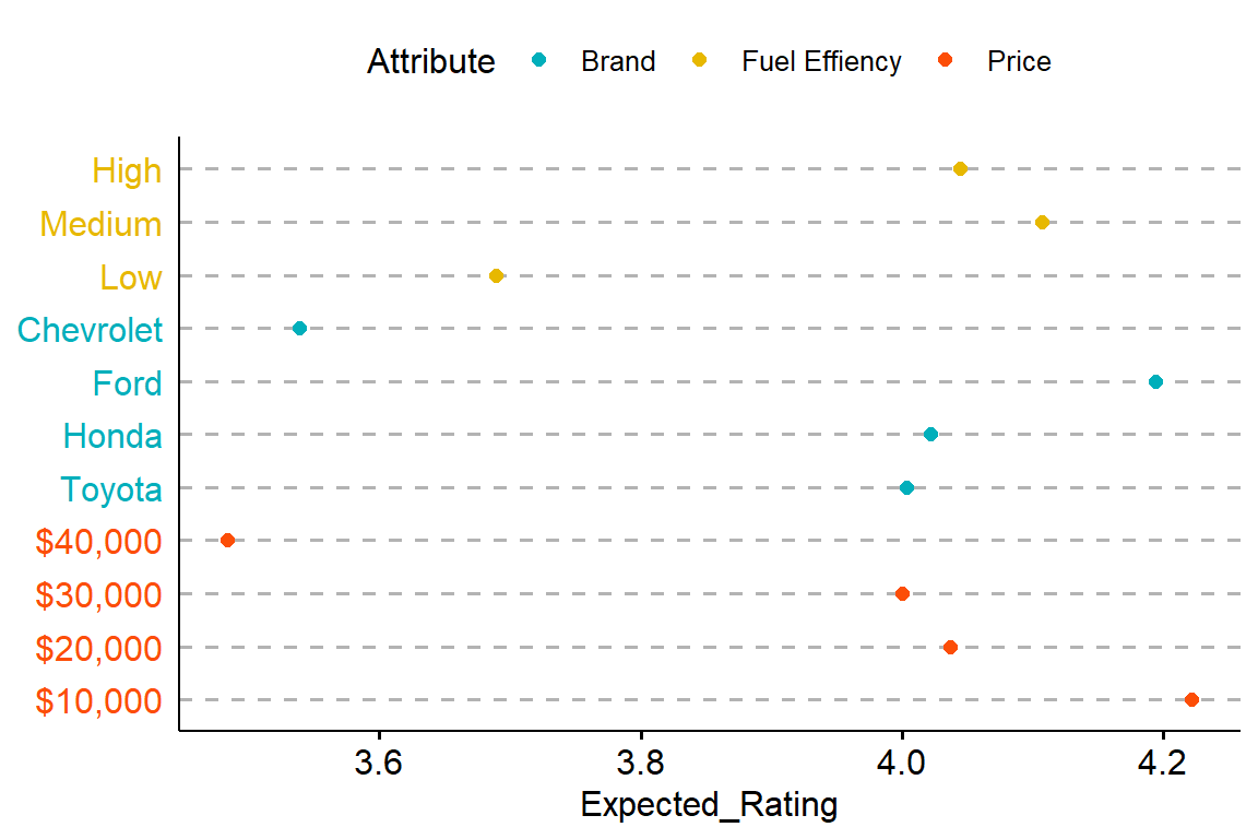
To better understand what are the levels within each attribute that have the biggest impact on rating we can plot the coefficients and/or calculate the marginal means for each level of each attribute and plot them.

Below we plot the average rating for each level of each attribute. In other words, we average the fitted values of the regression estimated above by each attribute.

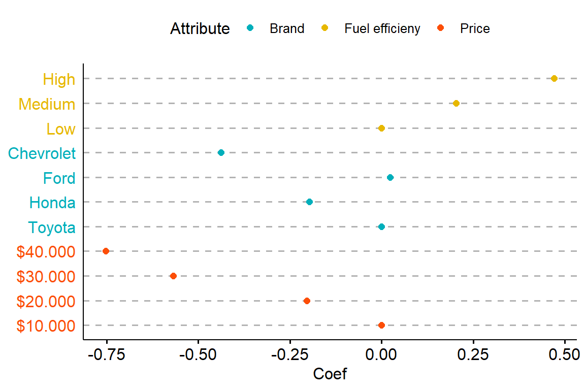
While here we plot the coefficients, which represent the relative change in rating with respect to the baseline.

5.2 MaxDiff Conjoint

MaxDiff Conjoint, also known as Best-Worst Scaling, is a technique used in market research to measure the relative importance or preference of different attributes or features of a product or service. It allows researchers to identify the most and least preferred attributes by asking respondents to choose the best and worst options from a set of alternatives. This approach helps uncover the trade-offs individuals make when making choices.

Experimental Design in MaxDiff Conjoint involves presenting respondents with a series of choice tasks or sets of alternatives. Each set consists of several attributes or features, and respondents are asked to indicate their best and worst choices within that set. By systematically varying the attributes across different choice sets, researchers can estimate the relative importance of each attribute based on the frequency of it being selected as the best or worst choice.

To make it easier to understand let’s make a practical example. We have four features and want to understand what is the preferred choice. Respondent are asked to select the best and worst feature among three possible alternatives (usually the number of alternatives for each block is between 3 and 5), the process is repeated t times. The alternatives displayed in each block are taken from balanced-incomplete-block-design which ensures that attributes are balanced (for each respondent all attributes appear the same number of times); orthogonal (for each respondent each pair of attributes appear the same number of times); randomized.

Here is the set of questions for the first individual:

library(ibd)
set.seed(123)
v <- 4 #Number of total attributes
b <- 5 #Number of questions, or experimental "blocks"
k <- 3 #Number of attributes per question 

ibd <- ibd(v = v, b = b, k = k) #Create design
ibd$design

##         [,1] [,2] [,3]
## Block-1    2    3    4
## Block-2    1    3    4
## Block-3    1    2    4
## Block-4    2    3    4
## Block-5    1    2    3

We collect data for N individuals, the final dataset is structured as follows: there are b blocks in total, and each block is represented by two separate sets. Each set consists of k rows (number of alternatives per question).

In the first set, there are three alternatives: 2, 3, and 4 (that corresponds to B, C, D). These alternatives are represented by three rows in the dataset. In each row, a value of 1 is present in the columns corresponding to the respective alternative. For example, in one row, a 1 appears in the Choice column for alternative D, indicating that D was chosen as the best option. In the second set, which follows the first set, there are three different alternatives. Instead of 1, each of these alternatives is represented by -1 to indicate the alternatives chosen as “worst”. In the dataset, specifically in the 5th row, a 1 appears in the Choice column for alternative B. This indicates that B was chosen as the worst option.

df.temp[df.temp$id==1&df.temp$block=="Block1", 3:7]

##   choice A  B  C  D
## 1      0 0  1  0  0
## 2      0 0  0  1  0
## 3      1 0  0  0  1
## 4      1 0 -1  0  0
## 5      0 0  0 -1  0
## 6      0 0  0  0 -1

Above are showed the data referring to the first block of the respondent, these fake data are generated for 300 individuals, with the following probabilities:

prob_mat2 <- data.frame(item = c("A", "B", "C", "D"), prob=c(0.2, 0.4, 0.05, 0.35))
prob_mat2

##   item prob
## 1    A 0.20
## 2    B 0.40
## 3    C 0.05
## 4    D 0.35

Now we can ask ourselves what is the most appropriate method to analyse the data. The easiest is to rely on a count based approach, we can: (i) count the relative frequencies each feature was selected as the Best vs. Worst. Dividing the number of times feature “x” has been selected by the number of times feature “x” appear in the question block (ii) Count the best feature for each respondent

calculate_percentage <- function(column, x=1) {
  percentage <- paste0(round(100 * sum(column == x&df.temp$choice==1) / sum(column == x), 0), " %")
  return(percentage)
}

# Apply the function to all columns of the dataframe
percentage_best <- apply(df.temp[,c("A", "B", "C", "D")], 2, calculate_percentage)
percentage_worst <- apply(df.temp[,c("A", "B", "C", "D")], 2, calculate_percentage, x=-1)

pct<-cbind(c("A", "B", "C", "D"), percentage_best, percentage_worst)
colnames(pct) <- c("Attribute", "Best %", "Worst %")
pct

##   Attribute Best % Worst %
## A "A"       "29 %" "35 %" 
## B "B"       "52 %" "24 %" 
## C "C"       "6 %"  "49 %" 
## D "D"       "45 %" "26 %"

With this approach attribute B is the best, followed by D, A and C.

We can use another approach and calculate the top feature choice for each respondent:

countA <- 0
countB <- 0
countC <- 0
countD <- 0


ids <- unique(df.temp$id)

for(i in 1:length(ids)){
  
  id_df <- subset(df.temp, df.temp$id==ids[i])
  
  temp_choice <- apply(id_df[,c("A", "B", "C", "D")], 2, function(column) sum(column == 1&id_df$choice==1) )
  
  if(names(which.max(temp_choice))=="A"){
    countA=countA+1
  }
  if(names(which.max(temp_choice))=="B"){
    countB=countB+1
  }
  if(names(which.max(temp_choice))=="C"){
    countC=countC+1
  }
  if(names(which.max(temp_choice))=="D"){
    countD=countD+1
  }
}

pct_resp <- data.frame(Attribute = c("A", "B", "C", "D"), 
                       Pct=c(paste0(100*countA/length(ids), " %"),paste0(100*countB/length(ids), " %"), 
                             paste0(100*countC/length(ids), " %"),paste0(100*countD/length(ids), " %")))
pct_resp

##   Attribute  Pct
## 1         A 16 %
## 2         B 56 %
## 3         C  1 %
## 4         D 27 %

This approach yields the same ranking as the previous, attribute B is the most chosen, followed by D, A and C.

A major drawback of count analysis is that it is unable to discern a rank ordering, B is the preferred choice with both methods but there’s nothing that ensures that in the set {B, A, D} D is preferred to B and thus leading to inconsistencies.
To overcome this issue we can employ a more sophisticated approach based on random utilities model. Random utility models (RUMs) are used to model individual decision-making in situations where people face choices between different alternatives. These models assume that individuals make choices based on the utility they derive from each alternative and that there is some randomness or variability involved in decision-making.

Here’s a simplified explanation of how random utility models work:

Utility of an Alternative:

Each alternative has an associated utility that represents the satisfaction or preference an individual derives from choosing that alternative. Utility is subjective and can vary from person to person.

Deterministic Utility:

The deterministic utility of an alternative is the component that captures the systematic or predictable factors influencing utility. It is typically represented as a linear combination of attribute values or characteristics of the alternatives.

Random Utility:

The random utility component captures the unobservable or random factors that influence utility and introduce variability in decision-making. It represents individual-specific preferences, taste variations, or random noise. Random utility is usually assumed to follow a specific distribution, often the Gumbel distribution in the case of discrete choice models.

Choice Probability:

The probability that an individual chooses a particular alternative is derived from the random utility associated with each alternative. The choice probability (P) for an alternative is typically calculated using the logit or conditional logit model. The probability of choosing alternative A, among alternatives A, B, C, D, …, can be expressed as: $P(A)=\frac{\exp(U(A))}{\sum_{i\in\{A, B, C, D, ...\}} exp(U(i))}$

Choosing the Alternative:

Based on the choice probabilities, an individual’s choice is determined by a probabilistic mechanism. The alternative with the highest choice probability has the highest likelihood of being selected.

Conditional logit model is specified as follows: \[\begin{equation} U_{j}=Z_{j}\beta_{j}+\epsilon_{i,j} \end{equation}\] where j indicates the alternative, the utilities in this specification varies only by the characteristic of the option. We thus have that option j is chosen over option l when: $U_{j}>U_{l}$ that implies $Z_{j}\beta_{j}+\epsilon_{j}>Z_{l}\beta_{l}+\epsilon_{l}$ that is: $\epsilon_{l}<Z_{j}\beta_{j}-Z_{l}\beta_{l}+\epsilon_{j}$. In general if we have J choices we have J-1 inequalities: \[\begin{equation} \epsilon_{l}<Z_{j}\beta_{j}-Z_{l}\beta_{l}+\epsilon_{j} \end{equation}\] \[\begin{equation} \epsilon_{m}<Z_{j}\beta_{j}-Z_{m}\beta_{m}+\epsilon_{j} \end{equation}\] \[\begin{equation} \epsilon_{n}<Z_{j}\beta_{j}-Z_{n}\beta_{n}+\epsilon_{j} \end{equation}\]

Therefore, generally, the probability that option j is selected equals: \[\begin{equation} P(\epsilon_{l}<Z_{j}\beta_{j}-Z_{l}\beta_{2}+\epsilon_{j} \cap \epsilon_{m}<Z_{j}\beta_{j}-Z_{m}\beta_{3}+\epsilon_{j} \cap ...) \end{equation}\]

Recall that if r. variables are independent than: $P(A \cap B \cap C \cap ...)=P(A)P(B)P(C)...$, since the errors ($\epsilon$) are assumed to be independent, the equation becomes: \[\begin{equation} P(Z_{j}\beta_{j}-Z_{l}\beta_{l}+\epsilon_{j})P(Z_{j}\beta_{j}-Z_{m}\beta_{m}+\epsilon_{j})... \end{equation}\]

Note that this probability is conditional on the value of $\epsilon_{j}$, to obtain the unconditional probability (which depends only on the coefficients $\beta$) we have to integrate out the random variable $\epsilon_{j}$ and finally we end up with the following equation: \[\begin{equation} \int P(Z_{j}\beta_{j}-Z_{l}\beta_{l}+\epsilon_{j})P(Z_{j}\beta_{j}-Z_{m}\beta_{m}+\epsilon_{j})...f_{j}(\epsilon_{j}) d\epsilon_{j} \end{equation}\]

Now the conditional logit model assumes that: (i) errors are independent; (ii) errors term follow a Gumbel distribution whose density function is $f(z)=\frac{1}{\theta}e\{-\frac{z}{\theta}\}e\{-e\{-\frac{z}{\theta}\}\}$ and finally (iii) errors are identically distributed.

With these assumption we can solve the above integral, obtaining an easy closed form solution: \[\begin{equation} P(Y=1|Z_{j})=\frac{\exp{(Z_{j}\beta_{j})}}{\sum_{l \in J} \exp{(Z_{l}\beta_{l})}} \end{equation}\]

These assumptions lead to the IIA Assumption, which states the odds ratio between any two alternatives in a choice set remains constant regardless of the presence or absence of other alternatives in the choice set. In other words, the relative preference for two alternatives should not be affected by the introduction or removal of irrelevant alternatives.

Let’s view it “mathematically”, if we have two alternatives j and l, the probability of them being chosen is, respectively, $P(Y=j)=\frac{\exp{(Z_{j}\beta_{j})}}{\sum_{i \in J} \exp{(Z_{i}\beta_{i})}}$ and $P(Y=l)=\frac{\exp{(Z_{l}\beta_{l})}}{\sum_{i \in J} \exp{(Z_{i}\beta_{i})}}$. The ratio of these two probabilities, which gives us how many times option i is preferred over option l is: \[\begin{equation} \frac{P(Y=j)}{P(Y=l)}=\frac{\exp{(Z_{j}\beta_{j})}}{\sum_{i \in J} \exp{(Z_{i}\beta_{i})}}\frac{\sum_{i \in J} \exp{(Z_{i}\beta_{i})}}{\exp{(Z_{l}\beta_{l})}}=\frac{\exp{(Z_{j}\beta_{j})}}{\exp{(Z_{l}\beta_{l})}} \end{equation}\]

This ratio for the two alternatives depends only on the characteristics of these two alternatives and not on those of other alternatives.

We can estimate this model via maximum likelihood. Given the data, the likelihood function, is: \[\begin{equation} Likelihood(z,\beta)=\prod_{i}\prod_{j}^{J} \left[ \frac{\exp{(Z_{j}\beta_{j})}}{\sum_{l \in J} \exp{(Z_{l}\beta_{l})}}\right]^{y_{ij}} \end{equation}\]

We have to omit an attribute, that will represent the baseline, in this example we set the attribute B to be the baseline.

### prepare the data 

alt1 <- as.data.frame(subset(df.temp, df.temp$alt==1))
alt2 <- as.data.frame(subset(df.temp, df.temp$alt==2))
alt3 <- as.data.frame(subset(df.temp, df.temp$alt==3))

### B is the baseline 

x1 <- alt1[c("A", "C", "D")]
y1 <- alt1["choice"]

x2 <- alt2[c("A", "C", "D")]
y2 <- alt2["choice"]

x3 <- alt3[c("A", "C", "D")]
y3 <- alt3["choice"]

x1 <- as.matrix(x1)
x2 <- as.matrix(x2)
x3 <- as.matrix(x3)


### log.likelihood function

ll.logit <- function(beta){
  
  LL <- exp(x1%*%beta)+exp(x2%*%beta)+exp(x3%*%beta)
  
  ll <- y1*log(exp(x1%*%beta)/LL)+y2*log(exp(x2%*%beta)/LL)+y3*log(exp(x3%*%beta)/LL)
  
  return(-sum(ll))
}

ini <- rep(0, ncol(x1))

## find maximum, hessian=T to recover SE 
opt <- optim(ini, ll.logit, method = "BFGS", hessian = TRUE)

p <- matrix(opt$par, nrow = ncol(x1), ncol = 1)
#rownames(p) <- colnames(x1)

names <- c("A", "C", "D")
output <- cbind(names, p, sqrt(diag(solve(opt$hessian))), p/sqrt(diag(solve(opt$hessian))))
colnames(output) <- c("Attribute", "Estimate", "Std. Error", "Z-value")
output

##      Attribute Estimate             Std. Error           Z-value            
## [1,] "A"       "-0.59268242618466"  "0.0604944158985362" "-9.79730802225998"
## [2,] "C"       "-1.23362652160386"  "0.0569535144525344" "-21.660235254349" 
## [3,] "D"       "-0.145214558205451" "0.0539417877212818" "-2.69206054044366"

The estimated parameters are all relative to the baseline B, that is set to 0. First of all the coefficients give us a clear rank ordering where $B>D>A>C$, we can further calculate the probability that alternative x is chosen among the set of all attributes computing the inverse logit transformation:

### convert in prob

probs <- c(exp(p[1])/(exp(p[1])+exp(p[2])+exp(p[3])+exp(0)), 
           exp(0)/(exp(p[1])+exp(p[2])+exp(p[3])+exp(0)), 
           exp(p[2])/(exp(p[1])+exp(p[2])+exp(p[3])+exp(0)), 
           exp(p[3])/(exp(p[1])+exp(p[2])+exp(p[3])+exp(0)))

names <- c("A", "B", "C", "D")

output_prob <- cbind(names, prob_mat$prob, round(probs,2))
colnames(output_prob) <- c("Attribute", "True Prob.", "Est. Prob.")
output_prob

##      Attribute True Prob. Est. Prob.
## [1,] "A"       "0.2"      "0.2"     
## [2,] "B"       "0.4"      "0.37"    
## [3,] "C"       "0.05"     "0.11"    
## [4,] "D"       "0.35"     "0.32"

Final remarks for practical applications: (i) Qualtrics suggest to run MaxDiff on 8-25 attributes (ii) 3-5 alternatives for each block (iii) No more than 15 sets