Chapter 7 Bootstrap
Bootstrap resampling is a statistical technique used to estimate the sampling distribution of a statistic by repeatedly resampling with replacement from an observed dataset. It was introduced by Bradley Efron in the late 1970s and has since become a crucial tool in statistical analysis, offering robust solutions to various estimation and hypothesis testing problems.
Procedure:
Original Dataset (D): Begin with a dataset containing N observations.
Resampling with Replacement: The core concept of bootstrap lies in generating multiple resamples of the same size as the original dataset. Resampling involves selecting observations from the dataset with replacement, effectively simulating a new dataset (D*) in each iteration.
Estimation: Calculate the desired statistic (mean, variance, median, etc.) for each resampled dataset (D*) to create a distribution of the statistic. This empirical distribution approximates the sampling distribution of the statistic under consideration.
Mathematical Foundation:
The bootstrap method capitalizes on the Law of Large Numbers. As the number of resamples approaches infinity, the empirical distribution of the statistic converges to the true sampling distribution. Mathematically, for a statistic θ, the bootstrap estimate θ* is given by:
\[\begin{equation} \theta{*}=g(D*) \end{equation}\]
where g(.) represents the calculation of the statistic of interest for a resampled dataset D*.
Let’s make a practical example base on the TURF analysis for which there is no (at least to my knowledge) analytical formula to recover the standard errors.
As seen in the first chapter Turf analysis yields in most of the cases sets that have very similar reach and it is unclear whether we should recommend a bundle over another based on the reach alone. In order to provide a more sound recommendation we can employ bootstrap to estimate which bundles are statistically different from each other.
Let’s load the data from, in total we have 10 columns, each corresponding to one of the tested items. Data or dichotomus, 1 means the respondent is willing to buy the item while 0 means she/he will not buy it. Here are the first 5 observations
##   item_1 item_2 item_3 item_4 item_5 item_6 item_7 item_8 item_9 item_10
## 1      0      0      0      0      0      0      1      0      1       1
## 2      0      0      1      1      0      0      1      1      1       1
## 3      0      1      0      0      0      1      1      0      1       1
## 4      0      1      1      0      0      0      1      1      1       1
## 5      0      0      1      0      1      1      1      1      1       1
Let’s calculate again the reach for each possible set of size 2.
##              item    share
## 1  item_9;item_10 98.33333
## 2  item_7;item_10 96.66667
## 3  item_8;item_10 96.66667
## 4   item_8;item_9 95.00000
## 5  item_4;item_10 94.44444
## 6   item_7;item_9 94.44444
## 7  item_5;item_10 93.88889
## 8  item_6;item_10 93.88889
## 9   item_7;item_8 93.88889
## 10 item_2;item_10 92.22222
The reach of the best 10 combinations is not greatly different from each other and is unclear whether this is difference is due to random chance or is there a clear preference for a bundle over another.
Remember the formula for calculating the reach is as follows \(Reach(x_{1}, x_{2})=\frac{\sum_{i=1}^{n} R(x_{1}, x_{2})}{n}\).
Applying bootstrap (to bundle (item_9; item_10)):
We draw N sample X* from the original dataset X with replacement (usually N=10000)
we calculate the reach for each of the bootstrap sample, ending up with N \(Reach(x_{1}, x_{2})*\) we thus have the complete distribution of the statistics for the bundle (item_9, item_10).
reach.bundle <- c()
N=5000
for(i in 1:N){

dt.boot <- dt[sample(1:nrow(dt), size = nrow(dt), replace = T),]
reach.bundle2 <- turf(dt.boot, c)
reach.temp <- reach.bundle2$share[reach.bundle2$item=="item_9;item_10"]
reach.bundle <- c(reach.bundle, reach.temp)

}

ggplot(data = NULL, aes(x = reach.bundle)) +
  geom_histogram(binwidth = 0.8, fill = "dodgerblue", color = "black", alpha = 0.8) +
  labs(title = "Reach: item_9; item_10", x = "Reach") +
  theme_minimal()+
  theme(plot.title = element_text(hjust=0.5))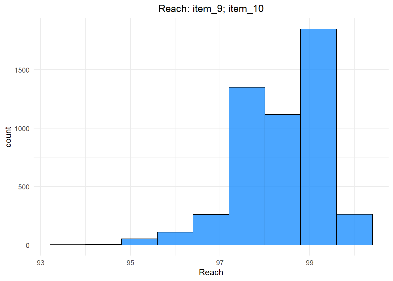
And we can thus calculate the 95% confidence interval (or whatever xx% confidence interval) in order to eventually perform statistical test to see what bundles have statistically different reach.
reach.bundle2 <- turf(dt, c)
og.reach <- reach.bundle2$share[reach.bundle2$item=="item_9;item_10"]

L.ci = quantile(reach.bundle - og.reach, .025)
U.ci = quantile(reach.bundle - og.reach, .975)
names(og.reach) <- "Mean"
c(og.reach - U.ci,og.reach, og.reach - L.ci)
## Mean Mean Mean
## 96.66667 98.33333 100.55556We can then calculate the 95% CI for each bundle of size 2.
## let's write a function that does it
bootstrap <- function(dt, N=1000, sample_size=nrow(dt), c){


  rex_ls <- list()


  for(i in 1:N){

    ## draw random sample
    sampled_dt <- dt[sample(nrow(dt), sample_size, replace = T), ]
    ## run turf
    rex_temp <- turf(sampled_dt, c)

    rex_ls <- append(rex_ls, list(rex_temp), after = (i-1))

  }


  #### merge
  merged_prova <- Reduce(function(x, y) merge(x, y, by = "item", all = TRUE), rex_ls)
  ### apply mean by row (should be approximately equal to rex_temp)
  rex_mean <- apply(merged_prova[,2:ncol(merged_prova)], 1, mean)
  names(rex_mean) <- merged_prova$item

  ### apply sd by row to get standard error
  rex_sd <- apply(merged_prova[,2:ncol(merged_prova)], 1, sd)
  names(rex_sd) <- merged_prova$item

  ### get CI
  rex <- turf(dt, c)
  mergeCI <- merge(rex, merged_prova, by = "item")

  L.re <- c()
  U.re <- c()

  for(i in 1:nrow(mergeCI)){
    diff <- mergeCI[i, 3:ncol(mergeCI)]-mergeCI[i,2]
    l.re <- quantile(diff, 0.025)
    u.re <- quantile(diff, 0.975)

    low_ci <- mergeCI[i,2]-u.re
    up_ci <- mergeCI[i,2]-l.re
    L.re <- c(L.re, low_ci)
    U.re <- c(U.re, up_ci)
  }


  rex_output <- data.frame(item = names(rex_sd), share = mergeCI$share, se = rex_sd,
                           low_ci = as.numeric(L.re), up_ci = as.numeric(U.re))

  return(rex_output)

}

reach.boot <- bootstrap(dt,N=1000, c=c)
rownames(reach.boot) <- NULL
reach.boot <- reach.boot[order(reach.boot$share, decreasing=T),]
head(reach.boot, 10)
## item share se low_ci up_ci
## 45 item_9;item_10 98.33333 0.9745866 96.66667 100.55556
## 40 item_7;item_10 96.66667 1.3402288 94.44444 99.44444
## 43 item_8;item_10 96.66667 1.3434330 94.44444 99.44444
## 44 item_8;item_9 95.00000 1.6119077 92.22222 98.33333
## 25 item_4;item_10 94.44444 1.7018566 91.66667 98.33333
## 42 item_7;item_9 94.44444 1.6237948 91.66667 97.77778
## 31 item_5;item_10 93.88889 1.7655835 90.55556 97.22222
## 36 item_6;item_10 93.88889 1.7453400 90.55556 97.22222
## 41 item_7;item_8 93.88889 1.7351509 90.55556 97.22222
## 10 item_2;item_10 92.22222 1.9233735 88.88889 95.55556Above are the 10 best combinations along with the SE and the CIs, we can see that there is a statistical significant difference only between the first and the tenth bundle.