Chapter 4 Poisson Regression

4.1 Learning Objectives

After finishing this chapter, you should be able to:

• Describe why simple linear regression is not ideal for Poisson data.
• Write out a Poisson regression model and identify the assumptions for inference.
• Write out the likelihood for a Poisson regression and describe how it could be used to estimate coefficients for a model.
• Interpret estimated coefficients from a Poisson regression and construct confidence intervals for them.
• Use deviances for Poisson regression models to compare and assess models.
• Use an offset to account for varying effort in data collection.
• Fit and use a zero-inflated Poisson (ZIP) model.

4.2 Introduction to Poisson Regression

Consider the following questions:

1. Are the number of motorcycle deaths in a given year related to a state’s helmet laws?
2. Does the number of employers conducting on-campus interviews during a year differ for public and private colleges?
3. Does the daily number of asthma-related visits to an Emergency Room differ depending on air pollution indices?
4. Has the number of deformed fish in randomly selected Minnesota lakes been affected by changes in trace minerals in the water over the last decade?

Each example involves predicting a response using one or more explanatory variables, although these examples have response variables that are counts per some unit of time or space. A Poisson random variable is often used to model counts; see Chapter 3 for properties of the Poisson distribution. Since a Poisson random variable is a count, its minimum value is zero and, in theory, the maximum is unbounded. We’d like to model our main parameter \(\lambda\), the average number of occurrences per unit of time or space, as a function of one or more covariates. For example, in the first question above, \(\lambda_i\) represents the average number of motorcycle deaths in a year for state \(i\), and we hope to show that state-to-state variability in \(\lambda_i\) can be explained by state helmet laws.

For an OLS linear regression model, the parameter of interest is the average response, \(\mu_i\), for subject \(i\), and \(\mu_i\) is modeled as a line in the case of one explanatory variable. By analogy, it might seem reasonable to try to model the Poisson parameter \(\lambda_i\) as a linear function of an explanatory variable but there are some problems with this approach. In fact, a model like \(\lambda_i=\beta_0+\beta_1x_i\) doesn’t work well for Poisson data. A line is certain to yield negative values for certain \(x_i\), but \(\lambda_i\) can only take on values from 0 to \(\infty\). In addition, the equal variance assumption in linear regression inference is violated because as the mean rate for a Poisson variable increases the variance also increases (recall from Chapter 3 that, if \(Y\) is the observed count, then \(E(Y)=Var(Y)=\lambda\)).

One way to avoid these problems is to model log(\(\lambda_i\)) instead of \(\lambda_i\) as a function of the covariates. The log(\(\lambda_i\)) takes on values from \(-\infty\) to \(\infty\). We can also take into account the increase in the variance with an increasing mean using this approach. (Note that throughout Broadening Your Statistical Horizons we use log to represent the natural logarithm.) Thus, we will consider the Poisson regression model:

\[\begin{equation} log(\lambda_i)=\beta_0+\beta_1 x_i \tag{4.1} \end{equation}\]

where the observed values \(Y_i \sim\) Poisson with \(\lambda=\lambda_i\) for a given \(x_i\). For example, each state \(i\) can potentially have a different \(\lambda\) depending on its value of \(x_i\), where \(x_i\) could represent presence or absence of a particular helmet law. Note that the Poisson regression model contains no separate error term like the \(\epsilon\) we see in linear regression, because \(\lambda\) determines both the mean and the variance of a Poisson random variable.

4.2.1 Poisson Regression Assumptions

Much like OLS, using Poisson regression to make inferences requires model assumptions.

1. Poisson Response The response variable is a count per unit of time or space, described by a Poisson distribution.
2. Independence The observations must be independent of one another.
3. Mean=Variance By definition, the mean of a Poisson random variable must be equal to its variance.
4. Linearity The log of the mean rate, log(\(\lambda\)), must be a linear function of x.

4.2.2 A Graphical Look at Poisson Regression

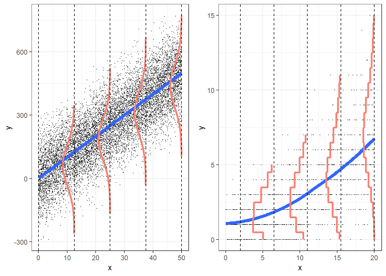
Figure 4.1: Regession Models: Linear Regression (left) and Poisson Regression (right)

Figure 4.1 illustrates a comparison of the OLS model for inference to Poisson regression using a log function of \(\lambda\).

1. The graphic displaying the ordinary least squares (OLS) inferential model appears in the left panel of Figure 4.1. It shows that for each level of X, the responses appear to be approximately normal. The panel on the right side of Figure 4.1 depicts what a Poisson regression model looks like. For each level of X, the responses follow a Poisson distribution (Assumption 1). For Poisson regression, small values of \(\lambda\) are associated with a distribution that is noticeably skewed with lots of small values and only a few larger ones. As \(\lambda\) increases the distribution of the responses begins to look more and more like a normal distribution.
2. In the OLS regression model, the variation in \(Y\) at each level of X, \(\sigma^2\), is the same. For Poisson regression the responses at each level of X become more variable with increasing means, where variance=mean (Assumption 3).
3. In the case of OLS, the mean responses for each level of X, \(\mu_{Y|X}\), fall on a line. In the case of the Poisson model, the mean values of \(Y\) at each level of \(X\), \(\lambda_{Y|X}\), fall on a curve, not a line, although the logs of the means should follow a line (Assumption 4).

4.3 Case Studies Overview

We take a look at the Poisson regression model in the context of three case studies. Each case study is based on real data and real questions. Modeling household size in the Philippines introduces the idea of regression with a Poisson response along with its assumptions. A quadratic term is added to a model to determine an optimal size per household, and methods of model comparison are introduced. The campus crime case study introduces two big ideas in Poisson regression modeling: offsets, to account for sampling effort, and overdispersion, when actual variability exceeds what is expected by the model. Finally, the weekend drinking example uses a modification of a Poisson model to account for more zeros than would be expected for a Poisson random variable. These three case studies also provide context for some of the familiar concepts related to modeling such as exploratory data analysis, estimation, and residual plots.

4.4 Case Study: Household Size in the Philippines

How many other people live with you in your home? The number of people sharing a house differs from country to country and often from region to region. International agencies use household size when determining needs of populations, and the household sizes determine the magnitude of the household needs.

The Philippine Statistics Authority (PSA) spearheads the Family Income and Expenditure Survey (FIES) nationwide. The survey, which is undertaken every three years, is aimed at providing data on family income and expenditure, including levels of consumption by item of expenditure. Our data, from the 2015 FIES, is a subset of 1500 of the 40,000 observations (Philippine Statistics Authority 2015). Our dataset focuses on five regions: Central Luzon, Metro Manila, Ilocos, Davao, and Visayas (see Figure 4.2).

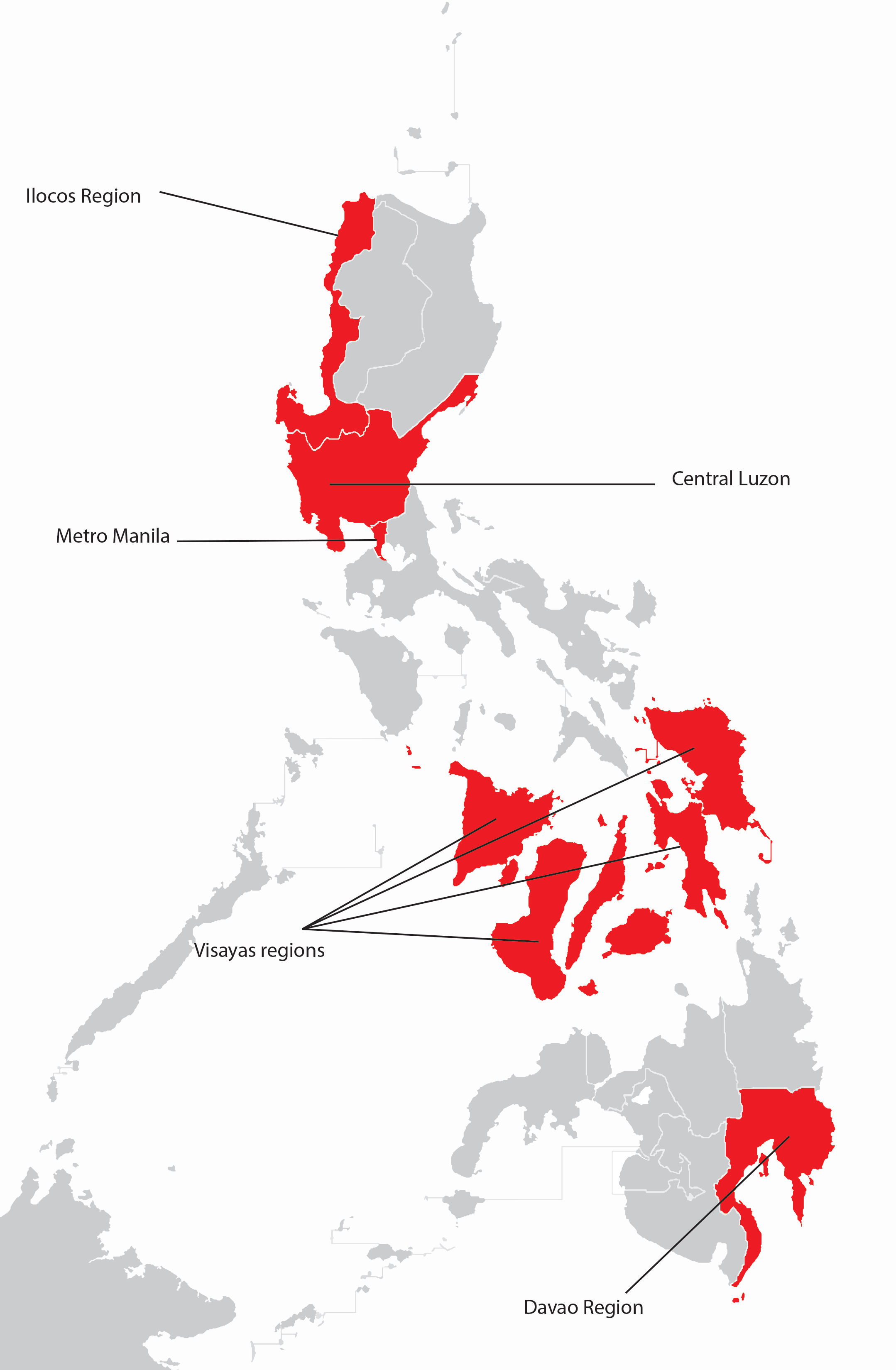
Figure 4.2: Regions of the Philippines

At what age are heads of households in the Philippines most likely to find the largest number of people in their household? Is this association similar for poorer households (measured by the presence of a roof made from predominantly light/salvaged materials)? We begin by explicitly defining our response, \(Y=\) number of people other than the head of the household. We then define the explanatory variables: age of the head of the household, type of roof (predominantly light/salvaged material or predominantly strong material), and location (Central Luzon, Davao Region, Ilocos Region, Metro Manila, or Visayas). Note that predominantly light/salvaged materials are a combination of light material, mixed but predominantly light material, and mixed but predominantly salvaged material, and salvaged matrial. Our response is a count, so we consider a Poisson regression where the parameter of interest is \(\lambda\), the average number of people, other than the head, per household. We will primarily examine the relationship between household size and age of the head of household, controlling for location and income.

4.4.1 Data Organization

The first five rows from our data set fHH1.csv are illustrated in Table 4.1. Each line of the data file refers to a household at the time of the survey:

• age = the age of the head of household
• numLT5 = the number in the household under 5 years of age
• total = the number of people in the household other than the head
• roof = the type of roof in the household (either Predominantly Light/Salvaged Material, or Predominantly Strong Material, where stronger material can sometimes be used as a proxy for greater wealth)
• location = where the house is located (Central Luzon, Davao Region, Ilocos Region, Metro Manila, or Visayas)

Table 4.1: The first five observations from the Philippines Household case study.

X1	location	age	total	numLT5	roof
1	CentralLuzon	65	0	0	Predominantly Strong Material
2	MetroManila	75	3	0	Predominantly Strong Material
3	DavaoRegion	54	4	0	Predominantly Strong Material
4	Visayas	49	3	0	Predominantly Strong Material
5	MetroManila	74	3	0	Predominantly Strong Material

4.4.2 Exploratory Data Analyses

For the rest of this case study, we will refer to the number of people in a household as the total number of people in that specific household besides the head of household. The average number of people in a household is 3.68 (Var = 5.53), and there are anywhere from 0 to 16 people in the house. Over 11.1% of these households are made from predominantly light and salvaged material. The mean number of people in a house for houses with a roof made from predominantly strong material is is 3.69 (Var=5.55), whereas houses with a roof made from predominantly light/salvaged material average 3.64 people (Var=5.41). Of the various locations, Visayas has the largest household size, on average, with a mean of 3.90 in the household, and the Davao Region has the smallest with a mean of 3.39.

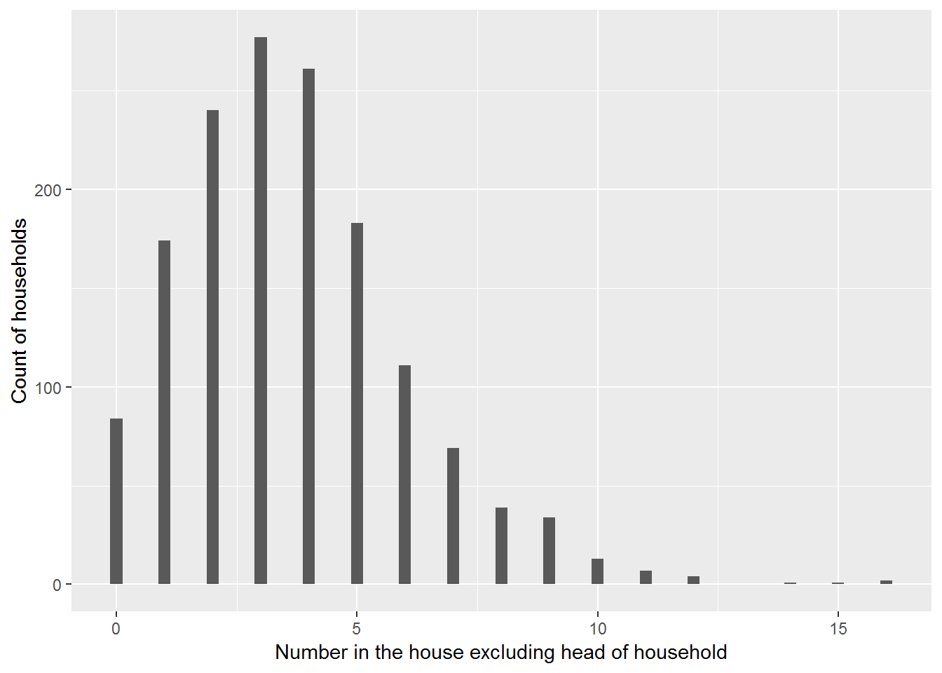
Figure 4.3: Philippines: Distribution of household size

Figure 4.3 reveals a fair amount of variability in the number in each house; responses range from 0 to 16 with many of the respondents reporting between 1 and 5 people in the house. Like many Poisson distributions, this graph is right skewed. It clearly does not suggest that the number of people in a household is a normally distributed response.

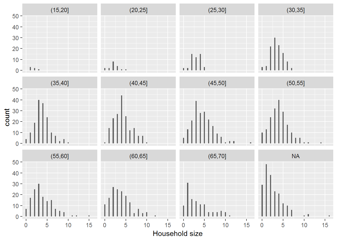
Figure 4.4: Distribution of household sizes by age group of the household head.

Figure 4.4 further shows that responses can be reasonably modeled with a Poisson distribution when grouped by a key explanatory variable: Age of the household head. These last two plots together suggest that Assumption 1 (Poisson Response) is satisfactory in this case study.

For Poisson random variables, the variance of \(Y\) (i.e., the square of the standard deviation of \(Y\)), is equal to its mean, where \(Y\) represents the size of an individual household. As the mean increases, the variance increases. So, if the response is a count and the mean and variance are approximately equal for each group of \(X\), a Poisson regression model may be a good choice. In Table 4.2 we display age groups by 5-year increments, to check to see if the empirical means and variances of the number in the house are approximately equal for each age group. This provides us one way in which to check the Poisson assumption.

Table 4.2: Compare mean and variance of household size within each age group

Age Groups	Mean	Variance	n
(15,20]	1.666667	0.6666667	6
(20,25]	2.166667	1.5588235	18
(25,30]	2.918367	1.4098639	49
(30,35]	3.444444	2.1931464	108
(35,40]	3.841772	3.5735306	158
(40,45]	4.234286	4.4447947	175
(45,50]	4.489691	6.3962662	194
(50,55]	4.010638	5.2512231	188
(55,60]	3.806897	6.5318966	145
(60,65]	3.705882	6.1958204	153
(65,70]	3.339130	7.9980168	115
NA	2.549738	5.5435657	191

If there is a problem with this assumption most often we see variances much larger than means. Here, as expected, we see more variability as age increases. However, it appears that the variance is smaller than the mean for lower ages, while the variance is greater than the mean for higher ages. Thus, there is some evidence of a violation of the mean=variance assumption (Assumption 3), although any violations are modest.

The Poisson regression model also implies that log(\(\lambda_i\)), not the mean household size \(\lambda_i\), is a linear function of age; i.e., \(log(\lambda_i)=\beta_0+\beta_1\textrm{age}_i\). Therefore, to check the linearity assumption (Assumption 4) for Poisson regression we would like to plot log(\(\lambda_i\)) by age. Unfortunately, \(\lambda_i\) is unknown. Our best guess of \(\lambda_i\) is the observed mean number in the household for each age (level of \(X\)). Because these means are computed for observed data, they are referred to as empirical means. Taking the logs of the empirical means and plotting by age provides a way to assess the linearity assumption. The smoothed curve added to Figure 4.5 suggests that there is a curvilinear relationship between age and the log of the mean household size, implying that adding a quadratic term should be considered. This finding is consistent with the researchers’ hypothesis that there is an age at which a maximum household size occurs. It is worth noting that we are not modeling the log of the empirical means, rather it is the log of the true rate that is modeled. Looking at empirical means, however, does provide an idea of the form of the relationship between log(\(\lambda)\) and \(x_i\).

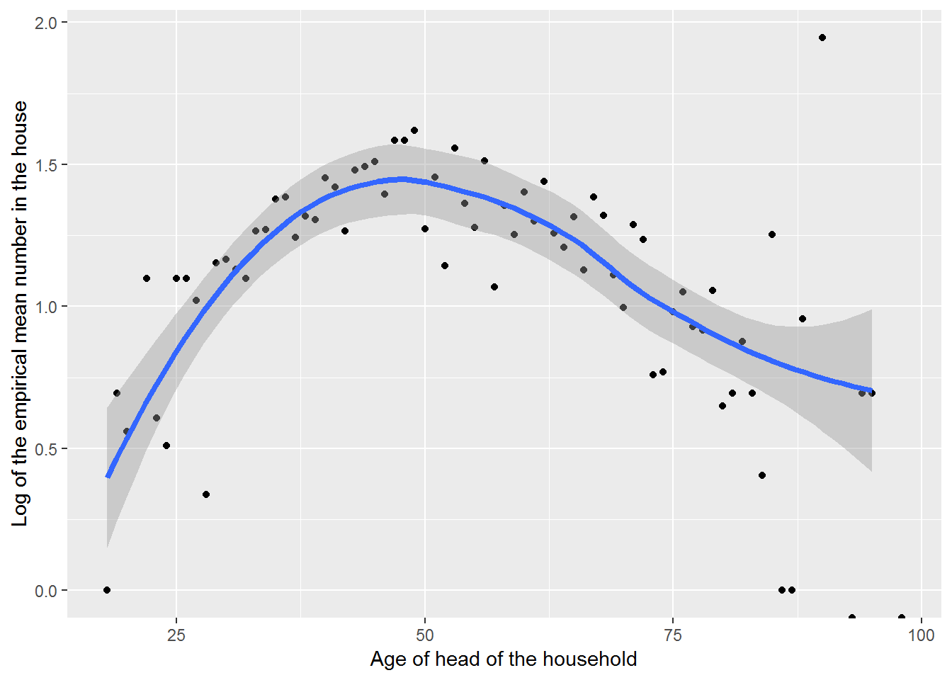
Figure 4.5: The log of the mean household sizes, besides the head of household, by age of the head of household, with loess smoother.

We can extend Figure 4.5 by fitting separate curves for each region (see Figure 4.6). This allows us to see if the relationship between mean household size and age is consistent across region. In this case, the relationships are pretty similar; if they weren’t we could consider adding an age-by-region interaction to our eventual Poisson regression model.

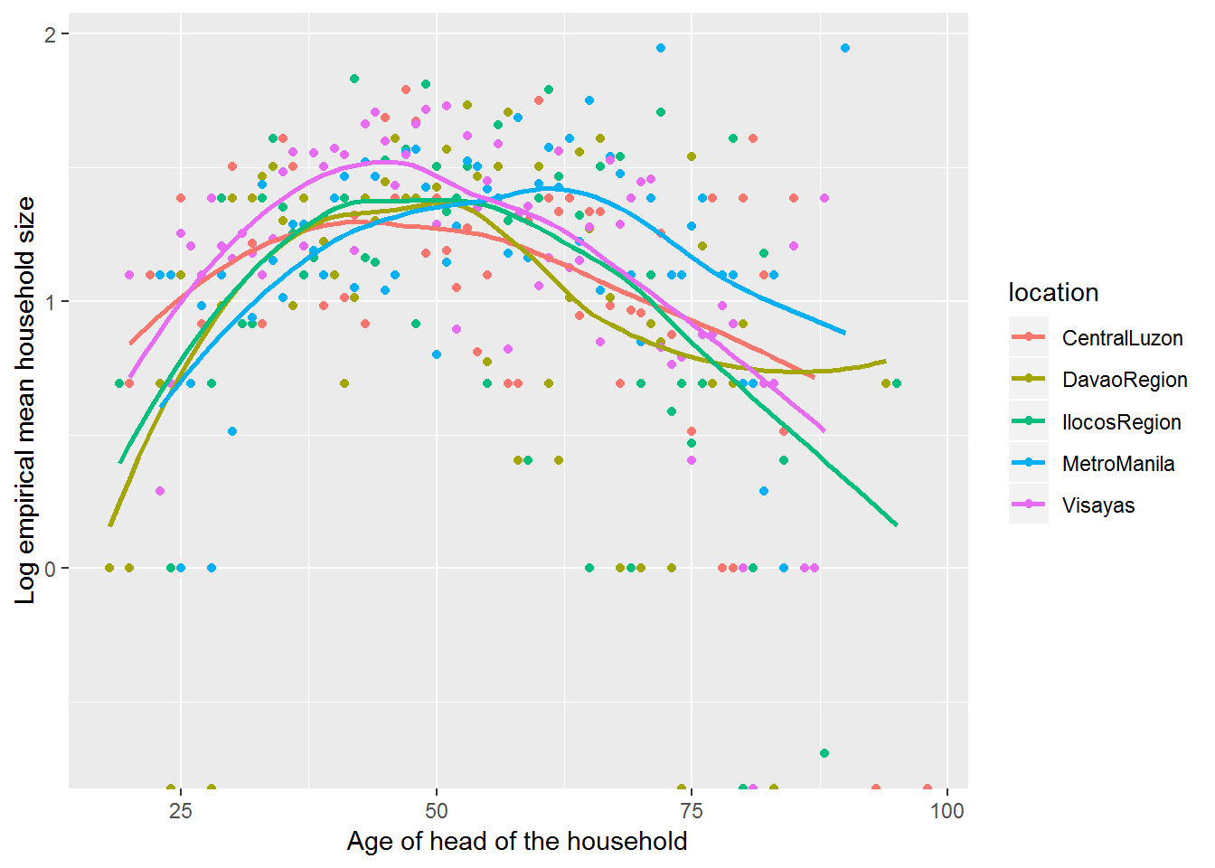
Figure 4.6: Empirical log of the mean household sizes vs. age of the head of household, with loess smoother by region.

Finally, the independence assumption (Assumption 2) can be assessed using knowledge of the study design and the data collection process. In this case, we do not have enough information to assess the independence assumption with the information we are given. If each household was not selected individually in a random manner, but rather groups of households were selected from different regions with differing customs about living arrangements, the independence assumption would be violated. If this were the case, we could use a multilevel model like those discussed in later chapters with a village term.

4.4.3 Estimation and Inference

We first consider a model for which log(\(\lambda\)) is linear in age. We then will determine whether a model with a quadratic term in age provides a significant improvement based on trends we observed in the exploratory data analysis.

R reports an estimated regression equation for the linear Poisson model as: \[ \widehat{log(\lambda)} = 1.55 - 0.0047 (age) \]

glm(formula = total ~ age, family = poisson, data = fHH1)

Coefficients:
              Estimate Std. Error z value Pr(>|z|)    
(Intercept)  1.5499422  0.0502754  30.829  < 2e-16 ***
age         -0.0047059  0.0009363  -5.026 5.01e-07 ***
---
(Dispersion parameter for poisson family taken to be 1)

    Null deviance: 2362.5  on 1499  degrees of freedom
Residual deviance: 2337.1  on 1498  degrees of freedom
AIC: 6714

How can the coefficient estimates be interpreted in terms of this example? As done when interpreting slopes in the OLS models, we consider how the estimated mean number in the house, \(\lambda\), changes as the age of the household head increases by an additional year. But in place of looking at change in the mean number in the house, with a Poisson regression we consider the log of the mean number in the house and then convert back to original units. For example, consider a comparison of two models—one for a given age (\(x\)) and one after increasing age by 1 (\(x+1\)) \[\begin{eqnarray} log(\lambda_X) &=& \beta_0 + \beta_1X \\ log(\lambda_{X+1}) &=& \beta_0 + \beta_1(X+1) \\ log(\lambda_{X+1})-log(\lambda_X) &= & \beta_1 \\ log \left(\frac{\lambda_{X+1}}{\lambda_X}\right) &= &\beta_1\\ \frac{\lambda_{X+1}}{\lambda_X} &=& e^{\beta_1} \tag{4.2} \end{eqnarray}\]

These results suggest that by exponentiating the coefficient on age we obtain the multiplicative factor by which the mean count changes. In this case, the mean number in the house changes by a factor of \(e^{-0.0047}=0.995\) or decreases by 0.5% with each additional year older the household head is; or, we predict a 0.47% increase in mean household size for a 1 year decrease in age of the household head (\(1/.995=1.0047\)). The quantity on the left hand side of Equation (4.2) is referred to as a rate ratio or relative risk, and it represents a percent change in the response for a unit change in X. In fact, for regression models in general, whenever a variable (response or explanatory) is logged, we make interpretations about multiplicative effects on that variable, while with unlogged variables we can reach our usual interpretations about additive effects.

Typically the standard errors for the estimated coefficients are included in Poisson regression output. Here the standard error for the estimated coefficient for age is 0.00094. We can use the standard error to construct a confidence interval for \(\beta_1\). A 95% CI provides a range of plausible values for the age coefficient and can be constructed: \[\hat\beta_1-Z^*\cdot SE(\hat\beta_1), \hat\beta_1+Z^*\cdot SE(\hat\beta_1)\] \[-0.0047-1.96*0.00094, -0.0047+1.96*0.00094\] \[ (-0.0065, -0.0029). \] Exponentiating the endpoints yields a confidence interval for the relative risk; i.e., the percent change in household size for each additional year older. Thus \((e^{-0.0065},e^{-0.0029})=(0.993,0.997)\) suggests that we are 95% confident that the mean number in the house decreases between 0.7% and 0.3% for each additional year older the head of household is. It is best to construct a confidence interval for the coefficient and then exponentiate the endpoints because the estimated coefficients more closely follow a normal distribution than the exponentiated coefficients. There are other approaches to constructing intervals in these circumstances, including profile likelihood, the delta method, and bootstrapping, and we will discuss some of those approaches later. In this case, for instance, the profile likelihood interval is nearly identical to the Wald-type (normal theory) confidence interval above.

# CI for betas using profile likelihood
confint(modela)

##                    2.5 %       97.5 %
## (Intercept)  1.451170100  1.648249185
## age         -0.006543163 -0.002872717

exp(confint(modela))

##                 2.5 %    97.5 %
## (Intercept) 4.2681057 5.1978713
## age         0.9934782 0.9971314

If there is no association between age and household size, there is no change in household size for each additional year, so \(\lambda_X\) is equal to \(\lambda_{X+1}\) and the ratio \(\lambda_{X+1}/\lambda_X\) is 1. In other words, if there is no association between age and household size, then \(\beta_1=0\) and \(e^{\beta_1}=1\). Note that our interval for \(e^{\beta_1}\), (0.993,0.997), does not include 1, so the model with age is preferred to a model without age; i.e., age is significantly associated with household size. Note that we could have similarly confirmed that our interval for \(\beta_1\) does not include 0 to show the significance of age as a predictor of household size.

Another way to test the significance of the age term is to calculate a Wald-type statistic. A Wald-type test statistic is the estimated coefficient divided by its standard error. When the true coefficient is 0, this test statistic follows a standard normal distribution for sufficiently large \(n\). The estimated coefficient associated with the linear term in age is \({\hat{\beta}_1}=-0.0047\) with standard error \(SE(\hat{\beta}_1)=0.00094\). The value for the Wald test statistic is then \(Z=\hat{\beta}_1/SE(\hat{\beta}_1)=-5.026\), where \(Z\) follows a standard normal distribution if \(\beta_1=0\). In this case, the two-sided p-value based on the standard normal distribution for testing \(H_0:\beta_1=0\) is almost 0 (\(p=0.000000501\)). In conclusion, we have statistically significant evidence (Z = -5.026, p < .001) that average household size decreases as age of the head of household increases.

4.4.4 Using Deviances to Compare Models

There is another way in which to assess how useful age is in the model. A deviance is a way in which to measure how the observed data deviates from the model predictions; it will be defined more precisely in Section 4.4.8, but it is similar to sum of squared errors (unexplained variability in the response) in OLS regression. Because we want models that minimize deviance, we calculate the drop-in-deviance when adding age to the model with no covariates (the null model). The deviances for the null model and the model with age can be found in the model output. A residual deviance for the model with age is reported as 2337.1 with 1498 df. The output also includes the deviance and degrees of freedom for the null model (2362.5 with 1499 df). The drop-in-deviance is 25.4 (2362.5 - 2337.1) with a difference of only 1 df, so that the addition of one extra term (age) reduced unexplained variability by 25.4. If the null model were true, we would expect the drop-in-deviance to follow a \(\chi^2\) distribution with 1 df. Therefore the p-value for comparing the null model to the model with age is found by determining the probability that the value for a \(\chi^2\) random variable with one degree of freedom exceeds 25.4, which is essentially 0. Once again, we can conclude that we have statistically significant evidence (\(\chi^2_{\text{df} =1}=25.4\), \(p < .001\)) that average household size decreases as age of the head of household increases.

# p-value for test comparing the null and first order models
# drop.in.dev <- modela$null.deviance - modela$deviance; drop.in.dev
# diff.in.df <- modela$df.null - modela$df.residual; diff.in.df
# 1-pchisq(drop.in.dev, diff.in.df)
model0 = glm(total~1,family=poisson,data=fHH1)
anova(model0, modela, test = "Chisq")

## Analysis of Deviance Table
## 
## Model 1: total ~ 1
## Model 2: total ~ age
##   Resid. Df Resid. Dev Df Deviance  Pr(>Chi)    
## 1      1499     2362.5                          
## 2      1498     2337.1  1   25.399 4.661e-07 ***
## ---
## Signif. codes:  0 '***' 0.001 '**' 0.01 '*' 0.05 '.' 0.1 ' ' 1

More formally, we are testing:

\[Null \ (reduced) \ Model: \log(\lambda) = \beta_0 \ or \ \beta_1=0\] \[Larger \ (full) \ Model: \log(\lambda) = \beta_0 + \beta_1(\textrm{age}) \ or \ \beta_1 \neq 0 \]

In order to use the drop-in-deviance test, the models being compared must be nested; i.e., all the terms in the smaller model must appear in the larger model. Here the smaller model is the null model with the single term \(\beta_0\) and the larger model has \(\beta_0\) and \(\beta_1\), so the two models are indeed nested. For nested models, we can compare the models’ residual deviances to determine whether the larger model provides a significant improvement.

Here, then, is a summary of these two approaches to hypothesis testing about terms in Poisson regression models:

Drop-in-deviance test to compare models

• Compute the deviance for each model, then calculate: drop-in-deviance = residual deviance for reduced model - residual deviance for the larger model.
• When the reduced model is true, the drop-in-deviance \(\sim \chi^2_d\) where d= the difference in the degrees of freedom associated with the two models (that is, the difference in the number of terms / coefficients).
• A large drop-in-deviance favors the larger model.

Wald test for a single coefficient

• Wald-type statistic = estimated coefficient / standard error
• When the true coefficient is 0, for sufficiently large \(n\), the test statistic \(\sim\) N(0,1).
• If the magnitude of the test statistic is large, there is evidence that the true coefficient is not 0.

The drop-in-deviance and the Wald-type tests usually provide consistent results; however, if there is a discrepancy the drop-in-deviance is preferred. Not only does the drop-in-deviance test perform better in more cases, but it’s also more flexible. If two models differ by one term, then the drop-in-deviance test essentially tests if a single coefficient is 0 like the Wald test does, while if two models differ by more than one term, the Wald test is no longer appropriate.

4.4.5 Using Likelihoods to fit Poisson Regression Models (Optional)

Before continuing with model building, we take a short detour to see how coefficient estimates are determined in a Poisson regression model. The least squares approach requires a linear relationship between the parameter, \(\lambda_i\) (the expected or mean response for observation \(i\)), and \(x_i\) (the age for observation \(i\)). However, it is log\((\lambda_i)\), not \(\lambda_i\), that is linearly related to X with the Poisson model. The assumptions of equal variance and normality also do not hold for Poisson regression. Thus, the method of least squares will not be helpful for inference in Poisson Regression. Instead of OLS, we employ the likelihood principle to find estimates of our model coefficients. We look for those coefficient estimates for which the likelihood of our data is maximized; these are the maximum likelihood estimates.

The likelihood for n independent observations is the product of the probabilities. For example, if we observe five households with household sizes of 4, 2, 8, 6, and 1 person beyond the head, the likelihood is: \[ Likelihood = P(Y_1=4)*P(Y_2=2)*P(Y_3=8)*P(Y_4=6)*P(Y_5=1)\] Recall that the probability of a Poisson response can be written \[P(Y=y)=\frac{e^{-\lambda}\lambda^y}{y!}\] for \(y = 0, 1, 2, ...\) So the likelihood can be written as \[\begin{eqnarray*} Likelihood&= &\frac{ e^{-\lambda_1}\lambda_1^4 }{ 4! }* \frac{ e^{-\lambda_2}\lambda_2^2 }{ 2! } *\frac{e^{-\lambda_3}\lambda_3^8}{8!}* \frac{e^{-\lambda_4}\lambda_4^6}{6!}*\frac{e^{-\lambda_5}\lambda_5^1}{1!}\\ \end{eqnarray*}\]

where each \(\lambda_i\) can differ for each household depending on a particular \(x_i\). As in chapter 2, it will be easier to find a maximum if we take the log of the likelihood and ignore the constant term resulting from the sum of the factorials:

\[\begin{eqnarray} -logL& \propto& \lambda_{1}-4log(\lambda_{1})+\lambda_{2}-2log(\lambda_{2}) \nonumber \\ & &+\lambda_{3}-8log(\lambda_{3})+\lambda_{4}-6log(\lambda_{4}) \nonumber \\ & &+\lambda_{5}-log(\lambda_{5}) \tag{4.3} \end{eqnarray}\]

Now if we had the age of the head of the household for each house (X), we consider the Poisson regression model: \[ log(\lambda_i)=\beta_0+\beta_1x_i \] This implies that \(\lambda\) differs for each age and can be determined using \[\lambda_i=e^{\beta_0+\beta_1x_i.}\]

If the ages are \(X=c(32,21,55,44,28)\) years, our loglikelihood can be written:

\[\begin{eqnarray} logL & \propto &[-e^{\beta_0+\beta_132}+4({\beta_0+\beta_132})]+ [-e^{\beta_0+\beta_121}+2({\beta_0+\beta_121})]+ \nonumber \\ & & [-e^{\beta_0+\beta_155}+8({\beta_0+\beta_155})]+ [-e^{\beta_0+\beta_144}+6({\beta_0+\beta_144})]+ \nonumber \\ & & [-e^{\beta_0+\beta_128}+({\beta_0+\beta_128})] \tag{4.4} \end{eqnarray}\]

To see this, match the terms in Equation (4.3) with those in Equation (4.4) noting that \(\lambda_i\) has been replaced with \(e^{\beta_0+\beta_1x_i}\). It is Equation (4.4) that will be used to estimate the coefficients \(\beta_0\) and \(\beta_1\). Although this looks a little more complicated than the loglikelihoods we saw in Chapter 2, the fundamental ideas are the same. In theory, we try out different possible values of \(\beta_0\) and \(\beta_1\) until we find the two for which the loglikelihood is largest. Most statistical software packages have automated search algorithms to find those values for \(\beta_0\) and \(\beta_1\) that maximize the loglikelihood.

4.4.6 Second Order Model

In Section 4.4.4, the Wald-type test and drop-in-deviance test both suggest that a linear term in age is useful. But our exploratory data analysis in Section 1.5 suggests that a quadratic model might be more appropriate. A quadratic model would allow us to see if there exists an age where the number in the house is, on average, a maximum. The output for a quadratic model appears below.

glm(formula = total ~ age + age2, family = poisson, data = fHH1)

Coefficients:
              Estimate Std. Error z value Pr(>|z|)    
(Intercept) -3.325e-01  1.788e-01  -1.859    0.063 .  
age          7.089e-02  6.890e-03  10.288   <2e-16 ***
age2        -7.083e-04  6.406e-05 -11.058   <2e-16 ***
---
(Dispersion parameter for poisson family taken to be 1)

    Null deviance: 2362.5  on 1499  degrees of freedom
Residual deviance: 2200.9  on 1497  degrees of freedom
AIC: 6579.8

We can assess the importance of the quadratic term in two ways. First, the p-value for the Wald-type statistic for age\(^2\) is statistically significant (Z = -11.058, p < 0.001). Another approach is to perform a drop-in-deviance test.

# p-value for test comparing the null and first order models
# drop.in.dev <- modela$deviance - modela2$deviance; drop.in.dev
# diff.in.df <- modela$df.residual - modela2$df.residual; diff.in.df
# 1-pchisq(104.78, 1)
anova(modela, modela2, test = "Chisq")

## Analysis of Deviance Table
## 
## Model 1: total ~ age
## Model 2: total ~ age + age2
##   Resid. Df Resid. Dev Df Deviance  Pr(>Chi)    
## 1      1498     2337.1                          
## 2      1497     2200.9  1   136.15 < 2.2e-16 ***
## ---
## Signif. codes:  0 '***' 0.001 '**' 0.01 '*' 0.05 '.' 0.1 ' ' 1

\(H_0\): log(\(\lambda\))=\(\beta_0+\beta_1age\) (reduced model)

\(H_A:\) log(\(\lambda\))=\(\beta_0+\beta_1age + \beta_2age^2\) (larger model)

The first order model has a residual deviance of 2337.1 with 1498 df and the second order model, the quadratic model, has a residual deviance of 2200.9 with 1497 df. The drop-in-deviance by adding the quadratic term to the linear model is 2337.1 - 2200.9 = 136.2 which can be compared to a \(\chi^2\) distribution with one degree of freedom. The p-value is esentially 0, so the observed drop of 136.2 again provides significant support for including the quadratic term.

We now have an equation in age which yields the estimated log(mean number in the house).
\[ \textrm{log(mean numHouse)} = -0.333 + 0.071(\textrm{age}) - 0.00071 (\textrm{age^2}) \]

As shown in the following, with calculus we can determine that the maximum estimated additional number in the house is \(e^{1.608} = 4.996\) when the head of the household is 50.328 years old.

\[\begin{eqnarray} \textrm{log(total)} & = & -0.333 + 0.071(\textrm{age}) - 0.00071 (\textrm{age^2}) \\ \frac{d}{d\textrm{age}}\textrm{log(total)} & = & 0 + 0.071 - 0.0014 (\textrm{age}) = 0 \\ (\textrm{age}) & = & 50.04 \\ \textrm{max[log(total)]} & = & -0.333 + 0.071 \times 50.04 - 0.00071 \times (50.04)^2 = 1.608 \end{eqnarray}\]

4.4.7 Adding a covariate

We should consider other covariates that may be related to household size. By controlling for important covariates, we can obtain more precise estimates of the relationship between age and household size. In addition, we may discover that the relationship between age and household size may differ by levels of a covariate. One important covariate to consider is location. As described earlier in the case study, there are 5 different regions that are associated with the Location variable: Central Luzon, Metro Manila, Visayas, Davao Region, and Ilocos Region. Assessing the utility of including the covariate Location is, in essence, comparing two nested models; here the quadratic model is compared to the quadratic model plus terms for Location. Results from the fitted model appears below; note that the Central Luzon is the reference region that all other regions are compared to.

glm(formula = total ~ age + age2 + location, family = poisson, 
    data = fHH1)

Coefficients:
                       Estimate Std. Error z value Pr(>|z|)    
(Intercept)          -0.3843338  0.1820919  -2.111  0.03480 *  
age                   0.0703628  0.0069051  10.190  < 2e-16 ***
age2                 -0.0007026  0.0000642 -10.944  < 2e-16 ***
locationDavaoRegion  -0.0193872  0.0537827  -0.360  0.71849    
locationIlocosRegion  0.0609820  0.0526598   1.158  0.24685    
locationMetroManila   0.0544801  0.0472012   1.154  0.24841    
locationVisayas       0.1121092  0.0417496   2.685  0.00725 ** 
---
(Dispersion parameter for poisson family taken to be 1)

    Null deviance: 2362.5  on 1499  degrees of freedom
Residual deviance: 2187.8  on 1493  degrees of freedom
AIC: 6574.7

Our Poisson regression model now looks like: \[\begin{eqnarray} \textrm{log(total)} & = & -0.384 + 0.070 \cdot \textrm{age} - 0.00070 \cdot \textrm{age}^2 +0.061 \cdot \textrm{IlocosRegion} + \\ & & 0.054 \cdot\textrm{MetroManila} +0.112 \cdot\textrm{Visayas} - 0.019 \cdot \textrm{DavaoRegion} \end{eqnarray}\]

Notice that because there are 5 different locations, we must represent the effects of different locations through 4 indicator variables. For example, \(\hat{\beta}_6=-0.0194\) indicates that, after controlling for the age of the head of household, the log mean household size is 0.0194 lower for households in the Davao Region than for households in the reference location of Central Luzon. In more interpretable terms, mean household size is \(e^{-0.0194}=0.98\) times “higher” (i.e., 2% lower) in the Davao Region than in Central Luzon, when holding age constant.

anova(modela2,modela2L, test="Chisq")

## Analysis of Deviance Table
## 
## Model 1: total ~ age + age2
## Model 2: total ~ age + age2 + location
##   Resid. Df Resid. Dev Df Deviance Pr(>Chi)  
## 1      1497     2200.9                       
## 2      1493     2187.8  4   13.144  0.01059 *
## ---
## Signif. codes:  0 '***' 0.001 '**' 0.01 '*' 0.05 '.' 0.1 ' ' 1

To test if the mean household size significantly differs by location, we must use a drop-in-deviance test, rather than a Wald-type test, because four terms (instead of just one) are added when including the location variable. From the Analysis of Deviance table above, adding the four terms corresponding to location to the quadratic model with age produces a statistically significant improvement \((\chi^2=13.144, df = 4, p=0.0106)\), so there is significant evidence that mean household size differs by location, after controlling for age of the head of household. Further modeling (not shown) shows that after controlling for location and age of the head of household, mean household size did not differ between the two types of roofing material.

4.4.8 Residuals for Poisson Models (Optional)

Residual plots may provide some insight into Poisson regression models, especially linearity and outliers, although the plots are not quite as useful here as they are for OLS. There are a few options for computing residuals and predicted values. Residuals may have the form of residuals for OLS models or the form of deviance residuals which, when squared, sum to the total deviance for the model. Predicted values can be estimates of the counts, \(e^{\beta_0+\beta_1X}\), or log counts, \(\beta_0+\beta_1X\). We will typically use the deviance residuals and predicted counts.

The residuals for OLS in simple linear regression have the form: \[\begin{eqnarray} OLS\hspace{2mm}residual_i &= &obs_i - fit_i \nonumber \\ &=&{Y_i-\hat{\mu}_i} \nonumber \\ &= &Y_i-(\hat{\beta}_0 +\hat{\beta}_1 X_i) \tag{4.5} \end{eqnarray}\] Residual sum of squares (RSS) are formed by squaring and adding these residuals, and we generally seek to minimize RSS in model building. We have several options for creating residuals for Poisson regression models. One is to create residuals in much the same way as we do in OLS. For Poisson residuals, the predicted values are denoted by \(\hat{\lambda}_i\) (in place of \(\hat{\mu}_i\) in Equation (4.5)); they are then standardized by dividing by the standard error, \(\sqrt{\hat{\lambda}_i}\). These kinds of residuals are referred to as Pearson residuals. \[\begin{equation} \textrm{Pearson residual}_i = \frac{Y_i-\hat{\lambda}_i}{\sqrt{\hat{\lambda}_i}} \tag{4.6} \end{equation}\]

Pearson residuals have the advantage that you are probably familiar with their meaning and the kinds of values you would expect. For example, after standardizing we expect most Pearson residuals to fall between -2 and 2. However, deviance residuals have some useful properties that make them a better choice for Poisson regression.

First, we define a deviance residual for an observation from a Poisson regression, \[\begin{equation} \textrm{deviance residual}_i = sign(Y_i-\hat{\lambda}_i) \sqrt{ 2 \left[Y_i log\left(\frac{Y_i}{\hat{\lambda}_i}\right) -(Y_i - \hat{\lambda}_i) \right]} \tag{4.7} \end{equation}\]

As its name implies, a deviance residual describes how the observed data deviates from the fitted model. Squaring and summing the deviances for all observations produces the residual deviance \(=\sum (\textrm{deviance residual})^2_i\). Relatively speaking, observations for good fitting models will have small deviances; that is, the predicted values will deviate little from the observed. However, you can see that the deviance for an observation does not easily translate to a difference in observed and predicted responses as is the case with OLS models.

A careful inspection of the deviance formula reveals several places where the deviance compares \(Y\) to \(\hat{\lambda}\): the sign of the deviance is based on the difference between \(Y\) and \(\hat{\lambda}\), and under the radical sign we see the ratio \(Y/\hat{\lambda}\) and the difference \(Y -\hat{\lambda}\). When \(Y = \hat{\lambda}\), that is, when the model fits perfectly, the difference will be 0 and the ratio will be 1 (so that its log will be 0). So like the residuals in OLS, an observation that fits perfectly will not contribute to the sum of the squared deviances. This definition of a deviance depends on the likelihood for Poisson models. Other models will have different forms for the deviance depending on their likelihood.

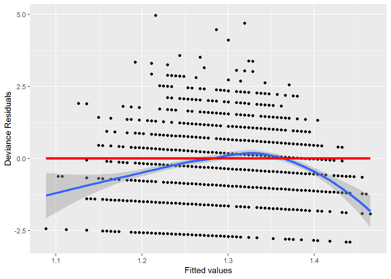
Figure 4.7: Residual plot for the Poisson model of household size by age of the household head

A plot (Figure 4.7) of the deviance residuals versus predicted responses for the first order model exhibits curvature, supporting the idea that the model may improved by adding a quadratic term. Other details related to residual plots can be found in a variety of sources including McCullagh and Nelder (1989).

4.4.9 Goodness-of-fit

The model residual deviance can be used to assess the degree to which the predicted values differ from the observed. When a model is true, we can expect the residual deviance to be distributed as a \(\chi^2\) random variable with degrees of freedom equal to the model’s residual degrees of freedom. Our model thus far, the quadratic terms for age plus the indicators for location, has a residual deviance of 2187.8 with 1493 df. The probability of observing a deviance this large if the model fits is esentially 0, saying that there is significant evidence of lack-of-fit.

1-pchisq(modela2$deviance, modela2$df.residual)  # GOF test

[1] 0

There are several reasons why lack-of-fit may be observed. We may be missing important covariates or interactions; a more comprehensive data set may be needed. There may be extreme observations that may cause the deviance to be larger than expected; however, our residual plots did not reveal any unusual points. Lastly, there may be a problem with the Poisson model. In particular, the Poisson model has only a single parameter, \(\lambda\), for each combination of the levels of the predictors which must describe both the mean and the variance. This limitation can become manifest when the variance appears to be larger than the corresponding means. In that case, the response is more variable than the Poisson model would imply, and the response is considered to be overdispered.

4.5 Least Squares Regression vs. Poisson Regression

\[ \underline{\textrm{Response}} \\ \mathbf{OLS:}\textrm{ Normal} \\ \mathbf{Poisson Regression:}\textrm{ counts} \\ \textrm{ } \\ \underline{\textrm{Variance}} \\ \mathbf{OLS:}\textrm{ Equal for each level of X} \\ \mathbf{Poisson Regression:}\textrm{ Equal to the mean for each level of X} \\ \textrm{ } \\ \underline{\textrm{Model Fitting}} \\ \mathbf{OLS:}\ \mu=\beta_0+\beta_1x \textrm{ using Least Squares}\\ \mathbf{Poisson Regression:}\ log(\lambda)=\beta_0+\beta_1x \textrm{ using Maximum Likelihood}\\ \textrm{ } \\ \underline{\textrm{EDA}} \\ \mathbf{OLS:}\textrm{ plot X vs. Y; add line} \\ \mathbf{Poisson Regression:}\textrm{ find }log(\bar{y})\textrm{ for several subgroups; plot vs. X} \\ \textrm{ } \\ \underline{\textrm{Comparing Models}} \\ \mathbf{OLS:}\textrm{ extra sum of squares F-tests; AIC/BIC} \\ \mathbf{Poisson Regression:}\textrm{ Drop in Deviance tests; AIC/BIC} \\ \textrm{ } \\ \underline{\textrm{Interpreting Coefficients}} \\ \mathbf{OLS:}\ \beta_1=\textrm{ change in }\mu_y\textrm{ for unit change in X} \\ \mathbf{Poisson Regression:}\ e^{\beta_1}=\textrm{ percent change in }\lambda\textrm{ for unit change in X} \]

4.6 Case Study: Campus Crime

Students want to feel safe and secure when attending a college or university. In response to legislation, the US Department of Education seeks to provide data and reassurances to students and parents alike. All postsecondary institutions that participate in federal student aid programs are required by the Jeanne Clery Disclosure of Campus Security Policy and Campus Crime Statistics Act and the Higher Education Opportunity Act to collect and report data on crime occurring on campus to the Department of Education. In turn, this data is publicly available on the website of the Office of Postsecondary Education. We are interested in looking at whether there are regional differences in violent crime on campus controlling for differences in the type of school.

4.6.1 Data Organization

Each row of c_data.csv contains crime information from a post secondary institution, either a college or university. The variables include:

• type = college (C) or university (U)
• region = region of the country (C = Central, MW = Midwest, NE = Northeast, SE = Southeast, SW = Southwest, and W = West)
• nv = the number of violent crimes for that institution for the given year
• Enrollment = enrollment at the school
• enroll1000 = enrollment at the school, in thousands
• nvrate = number of violent crimes per 1000 students

# A tibble: 10 x 6
   Enrollment type     nv nvrate enroll1000 region
        <dbl> <chr> <dbl>  <dbl>      <dbl> <chr> 
 1       5590 U        30 5.37         5.59 SE    
 2        540 C         0 0            0.54 SE    
 3      35747 U        23 0.643       35.7  W     
 4      28176 C         1 0.0355      28.2  W     
 5      10568 U         1 0.0946      10.6  SW    
 6       3127 U         0 0            3.13 SW    
 7      20675 U         7 0.339       20.7  W     
 8      12548 C         0 0           12.5  W     
 9      30063 U        19 0.632       30.1  C     
10       4429 C         4 0.903        4.43 C     

4.6.2 Exploratory Data Analysis

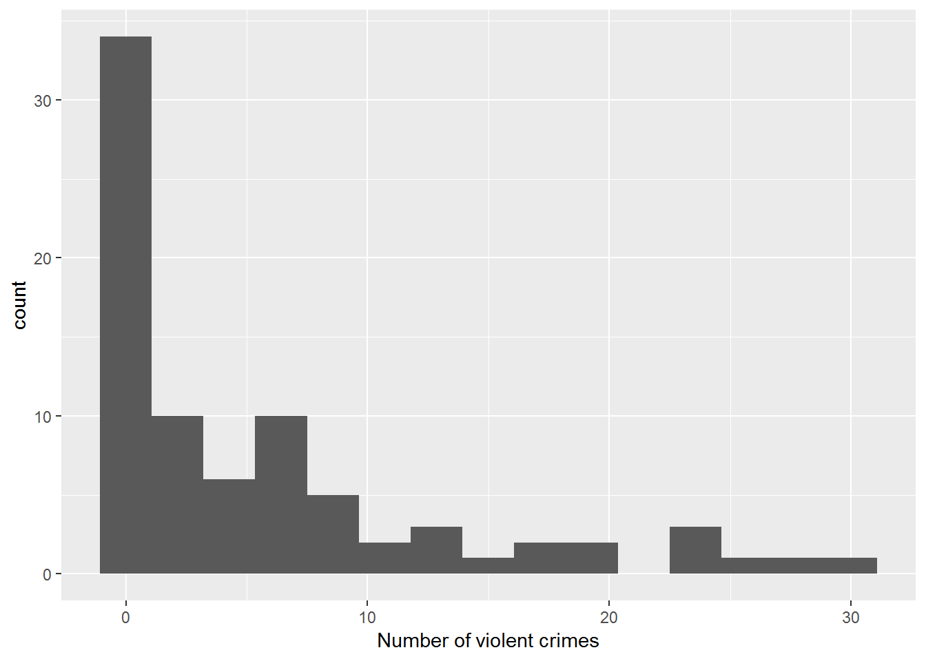
Figure 4.8: Histogram of number of violent crimes by institution

A graph of the number of violent crimes, Figure 4.8, reveals the pattern often found with distributions of counts of rare events. Many schools reported no violent crimes or very few crimes. A few schools have a large number of crimes making for a distribution that appears to be far from normal. Therefore, Poisson regression should be used to model our data; Poisson random variables are often used to represent counts (e.g., number of violent crimes) per unit of time or space (e.g., one year).

Let’s take a look at the covariates of interest for these schools: type of institution and region. In our data, the majority of institutions are universities (65% of the 81 schools) and only 35% are colleges. Interest centers on whether the different regions tend to have different crime rates. Table 4.3 contains the name of each region and each column represents the percentage of schools in that region which are colleges or universities. The proportion of colleges varies from a low of 20% in the Southwest (SW) to a high of 50% in the West (W).

Table 4.3: Proportion of colleges and universities within region in the campus crime data set

	C	MW	NE	SE	SW	W
C	0.294	0.3	0.381	0.4	0.2	0.5
U	0.706	0.7	0.619	0.6	0.8	0.5

While a Poisson regression model is a good first choice because the responses are counts per year, it is important to note that the counts are not directly comparable because they come from different size schools. This issue sometimes is referred to as the need to account for sampling effort; in other words, we expect schools with more students to have more reports of violent crime since there are more students who could be affected. We cannot compare the 30 violent crimes from the first school in the data set to no violent crimes for the second school when their enrollments are vastly different; 5,590 for school 1 versus 540 for school 2. We can take the differences in enrollments into account by including an offset in our model, which we will discuss in the next section. For the remainder of the EDA, we examine the violent crime counts in terms of the rate per 1,000 enrolled \(\frac{\textrm{number of violent crimes}}{\textrm{number enrolled}} \cdot 1000\).

Note that there is a noticeable outlier for a Southeastern school (5.4 violent crimes per 1000 students), and there is an observed rate of 0 for the Southwestern colleges which can lead to some computational issues. We therefore combined the SW and SE to form a single category of the South, and we also removed the extreme observation from the data set.

Table 4.4: The mean and variance of the violent crime rate by region and type of institution

region	type	MeanCount	VarCount	MeanRate	VarRate	n
C	C	1.6000000	3.3000000	0.3979518	0.2780913	5
C	U	4.7500000	30.9318182	0.2219441	0.0349266	12
MW	C	0.3333333	0.3333333	0.0162633	0.0007935	3
MW	U	8.7142857	30.9047619	0.4019003	0.0620748	7
NE	C	6.0000000	32.8571429	1.1249885	1.1821000	8
NE	U	5.9230769	79.2435897	0.4359273	0.3850333	13
S	C	1.1250000	5.8392857	0.1865996	0.1047178	8
S	U	8.6250000	68.2500000	0.5713162	0.2778065	16
W	C	0.5000000	0.3333333	0.0680164	0.0129074	4
W	U	12.5000000	57.0000000	0.4679478	0.0246670	4

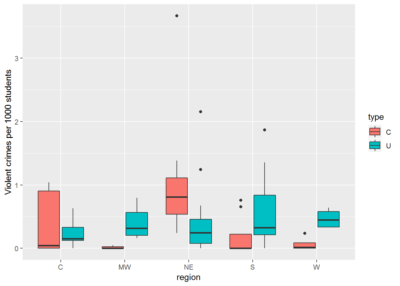
Figure 4.9: Boxplot of violent crime rate by region and type of institituion

Table 4.4 and Figure 4.9 display mean violent crime rates that are generally lower at the colleges within a region (with the exception of the Northeast). In addition, the regional pattern of rates at universities appears to differ from that of the colleges.

4.6.3 Accounting for Enrollment

Although working with the observed rates (per 1000 students) is useful during the exploratory data analysis, we do not use these rates explicitly in the model. The counts (per year) are the Poisson responses when modeling, so we must take into account the enrollment in a different way. Our approach is to include a term on the right side of the model called an offset, which is the log of the enrollment, in thousands. There is an intuitive heuristic for the form of the offset. If we think of \(\lambda\) as the mean number of violent crimes per year, then \(\lambda/1000\) represents the number per 1000 students, so that the yearly count is adjusted to be comparable across schools of different sizes. Adjusting the yearly count by enrollment is equivalent to adding \(log(\textrm{enroll1000})\) to the right hand side of the Poisson regression equation—essentially as a predictor with a fixed coefficient of 1:

\[\begin{eqnarray} log(\frac{\lambda}{\textrm{enroll1000}} )= \beta_0 + \beta_1(\textrm{type}) \nonumber \\ log(\lambda)-log(\textrm{enroll1000}) = \beta_0 + \beta_1(\textrm{type}) \nonumber \\ log(\lambda) = \beta_0 + \beta_1(\textrm{type}) + log(\textrm{enroll1000}) \end{eqnarray}\]

While this heuristic is helpful, it is important to note that it is not \(\frac{\lambda}{ \textrm{enroll1000}}\) that we are modeling. We are still modeling \(log(\lambda)\), but we’re adding an offset to adjust for differing enrollments, where the offset has the unusual feature that the coefficient is fixed at 1.0. As a result, no estimated coefficient for enroll1000 will appear in the output.

4.7 Modeling Assumptions

In Table 4.4, we see that the variances are greatly higher than the mean counts in almost every group. Thus, we have reason to question the Poisson regression assumption of variability equal to the mean; we will have to return to this issue after some initial modeling. The fact that the variance of the rate of violent crimes per 1000 students tends to be on the same scale as the mean tells us that adjusting for enrollment may provide some help, although that may not completely solve our issues with excessive variance.

As far as other model assumptions, linearity with respect to \(log(\lambda)\) is difficult to discern without continuous predictors, and it is not possible to assess independence without knowing how the schools were selected.

4.8 Initial Models

We are interested primarily in differences in violent crime between institutional types controlling for difference in regions, so we fit a model with both region and our offset. Note that the central region is the reference level in our model.

glm(formula = nv ~ type + region, family = poisson, data = c.data, 
    offset = log(enroll1000))

Coefficients:
            Estimate Std. Error z value Pr(>|z|)    
(Intercept) -1.54780    0.17114  -9.044  < 2e-16 ***
typeU        0.27956    0.13314   2.100   0.0358 *  
regionMW     0.09912    0.17752   0.558   0.5766    
regionNE     0.77813    0.15307   5.084 3.70e-07 ***
regionS      0.58238    0.14896   3.910 9.24e-05 ***
regionW      0.26275    0.18753   1.401   0.1612    
---
(Dispersion parameter for poisson family taken to be 1)

    Null deviance: 392.76  on 79  degrees of freedom
Residual deviance: 348.68  on 74  degrees of freedom
AIC: 573.32

From our model the Northeast and the South differ significantly from the Central region (p= 0.00000037 and p=0.0000924 respectively). The estimated coefficient of 0.778 means that the violent crime rate per 1,000 in the Northeast is nearly 2.2 (\(e^{0.778}\)) times that of the Central region controlling for the type of school. A wald-type confidence interval for this factor can be constructed by first calculating a CI for the coefficient (0.778 \(\pm\) \(1.96 \cdot 0.153\)) and then exponentiating (1.61 to 2.94).

4.8.1 Tukey’s Honestly Significant Differences

Comparisons to regions other than the Central region can be accomplished by changing the reference region. If many comparisons are made, it would be best to adjust for multiple comparisons using a method such as Tukey’s Honestly Significant Differences, which considers all pairwise comparisons among regions. This method helps control the large number of false positives that we would see if we ran multiple t-tests comparing groups. The honestly significant difference compares a standardized mean difference between two groups to a critical value from a studentized range distribution.

Multiple Comparisons of Means: Tukey Contrasts

Linear Hypotheses:
             Estimate Std. Error z value Pr(>|z|)    
MW - C == 0   0.09912    0.17752   0.558   0.9804    
NE - C == 0   0.77813    0.15307   5.084   <0.001 ***
S - C == 0    0.58238    0.14896   3.910   <0.001 ***
W - C == 0    0.26275    0.18753   1.401   0.6209    
NE - MW == 0  0.67901    0.15545   4.368   <0.001 ***
S - MW == 0   0.48327    0.15143   3.191   0.0118 *  
W - MW == 0   0.16364    0.18942   0.864   0.9079    
S - NE == 0  -0.19574    0.12182  -1.607   0.4863    
W - NE == 0  -0.51537    0.16587  -3.107   0.0158 *  
W - S == 0   -0.31963    0.16296  -1.961   0.2795    
---
(Adjusted p values reported -- single-step method)

In our case, Tukey’s Honestly Significant Differences simultaneously evaluates all 10 mean differences between pairs of regions. We find that the Northeast has significantly higher rates of violent crimes than the Central, Midwest, and Western regions, while the South has significantly higher rates of violent crimes than the Central and the Midwest, controlling for the type of institution. The University indicator is significant and, after exponentiating the coefficient, can be interpreted as an approximately (\(e^{0.280}\)) 32% increase in violent crime rate over colleges after controlling for region.

These results certainly suggest significant differences in regions and type of institution. However, the EDA findings suggest the effect of the type of institution may vary depending upon the region, so we consider a model with an interaction between region and type.

glm(formula = nv ~ type + region + region:type, family = poisson, 
    data = c.data, offset = log(enroll1000))

Coefficients:
               Estimate Std. Error z value Pr(>|z|)    
(Intercept)     -1.4741     0.3536  -4.169 3.05e-05 ***
typeU            0.1959     0.3775   0.519  0.60377    
regionMW        -1.9765     1.0607  -1.863  0.06239 .  
regionNE         1.5529     0.3819   4.066 4.77e-05 ***
regionS         -0.1562     0.4859  -0.322  0.74779    
regionW         -1.8337     0.7906  -2.319  0.02037 *  
typeU:regionMW   2.1965     1.0765   2.040  0.04132 *  
typeU:regionNE  -1.0698     0.4200  -2.547  0.01086 *  
typeU:regionS    0.8121     0.5108   1.590  0.11185    
typeU:regionW    2.4106     0.8140   2.962  0.00306 ** 
---
(Dispersion parameter for poisson family taken to be 1)

    Null deviance: 392.76  on 79  degrees of freedom
Residual deviance: 276.70  on 70  degrees of freedom
AIC: 509.33

These results provide convincing evidence of an interaction between the effect of region and the type of institution. A drop-in-deviance test like the one we carried out in the previous case study confirms the significance of the contribution of the interaction to this model. We have statistically significant evidence (\(\chi^2=71.98, df=4, p<.001\)) that the difference between colleges and universities in violent crime rate differs by region. For example, our model estimates that violent crime rates are 13.6 (\(e^{.196+2.411}\)) times higher in universities in the West compared to colleges, while in the Northeast we estimate that violent crime rates are 2.4 (\(\frac{1}{e^{.196-1.070}}\)) times higher in colleges.

Analysis of Deviance Table

Model 1: nv ~ type + region
Model 2: nv ~ type + region + region:type
  Resid. Df Resid. Dev Df Deviance  Pr(>Chi)    
1        74     348.68                          
2        70     276.70  4   71.981 8.664e-15 ***
---
Signif. codes:  0 '***' 0.001 '**' 0.01 '*' 0.05 '.' 0.1 ' ' 1

The residual deviance (276.70 with 70 df) suggests significant lack of fit in the interaction model (p < .001). One possibility is that there are other important covariates that could be used to describe the differences in the violent crime rates. Without additional covariates to consider, we look for extreme observations, but we have already eliminated the most extreme of the observations.

In the absence of other covariates or extreme observations, we consider overdispersion as a possible explanation of the significant lack-of-fit.

4.9 Overdispersion

4.9.1 Dispersion parameter adjustment

Overdispersion suggests that there is more variation in the response than the model implies. Under a Poisson model, we would expect the means and variances of the response to be about the same in various groups. Without adjusting for overdispersion, we use incorrect, artificially small standard errors leading to artificially small p-values for model coefficients. We may also end up with artificially complex models.

We can take overdispersion into account in several different ways. The simplest is to use an estimated dispersion factor to inflate standard errors. Another way is to use a negative-binomial regression model. We begin with using an estimate of the dispersion parameter.

We can estimate a dispersion parameter, \(\phi\), by dividing the model deviance by its corresponding degrees of freedom; i.e., \(\hat\phi=\frac{\sum(\textrm{Pearson residuals})^2}{n-p}\) where \(p\) is the number of model parameters. It follows from what we know about the \(\chi^2\) distribution that if there is no overdispersion, this estimate should be close to one. It will be larger than one in the presence of overdispersion. We inflate the standard errors by multiplying the variance by \(\phi\) so that the standard errors are larger than the likelihood approach would imply; i.e., \(SE_Q(\hat\beta)=\sqrt{\hat\phi}*SE(\hat\beta)\), where \(Q\) stands for “quasipoisson” since multiplying variances by \(\phi\) is an ad-hoc solution. Our process for model building and comparison is called quasilikelihood—similar to likelihood but without exact underlying distributions. If we choose to use a dispersion parameter with our model, we refer to the approach as quasilikelihood. The following output illustrates a quasipoisson approach to the interaction model:

glm(formula = nv ~ type + region + region:type, family = quasipoisson, 
    data = c.data, offset = log(enroll1000))

Coefficients:
               Estimate Std. Error t value Pr(>|t|)  
(Intercept)     -1.4741     0.7455  -1.977   0.0520 .
typeU            0.1959     0.7961   0.246   0.8063  
regionMW        -1.9765     2.2366  -0.884   0.3799  
regionNE         1.5529     0.8053   1.928   0.0579 .
regionS         -0.1562     1.0246  -0.152   0.8792  
regionW         -1.8337     1.6671  -1.100   0.2751  
typeU:regionMW   2.1965     2.2701   0.968   0.3366  
typeU:regionNE  -1.0698     0.8856  -1.208   0.2311  
typeU:regionS    0.8121     1.0771   0.754   0.4534  
typeU:regionW    2.4106     1.7164   1.404   0.1646  
---
(Dispersion parameter for quasipoisson family taken to be 4.446556)

    Null deviance: 392.76  on 79  degrees of freedom
Residual deviance: 276.70  on 70  degrees of freedom
AIC: NA

In the absence of overdispersion, we expect the dispersion parameter estimate to be 1.0. The estimated dispersion parameter here is much larger than 1.0 (4.447) indicating overdispersion (extra variance) that should be accounted for. The larger estimated standard errors in the quasipoisson model reflect the adjustment. For example, the standard error for the West region term from a likelihood based approach is 0.7906, whereas the quasilikelihood standard error is \(\sqrt{4.47}*0.7906\) or 1.6671. This term is no longer significant under the quasipoisson model. In fact, after adjusting for overdispersion (extra variation), none of the model coefficients in the quasipoisson model are significant at the .05 level! This is because standard errors were all increased by a factor of 2.1 (\(\sqrt{\hat\phi}=\sqrt{4.447}=2.1\)), while estimated coefficients remain unchanged.

Note that tests for individual parameters are now based on the t-distribution rather than a standard normal distribution, with test statistic \(t=\frac{\hat\beta}{SE_Q(\hat\beta)}\) following an (approximate) t-distribution with \(n-p\) degrees of freedom if the null hypothesis is true (\(H_O:\beta=0\)). Drop-in-deviance tests can be similarly adjusted for overdispersion in the quasipoisson model. In this case, you can divide the test statistic by the estimated dispersion parameter and compare the result to an F-distribution with the difference in the model degrees of freedom for the numerator and the degrees of freedom for the larger model in the denominator. That is, \(F=\frac{\textrm{drop in deviance}}{\hat\phi}\) follows an (approximate) F-distribution when the null hypothesis is true (\(H_O\): reduced model sufficient). The output below tests for an interaction between region and type of institution after adjusting for overdispersion (extra variance):

phi <- sum(resid(modeli, type='pearson')^2) / modeli$df.residual
drop.in.dev <- modeltr$deviance - modeli$deviance
diff.in.df <- modeltr$df.residual - modeli$df.residual
Fstat <- drop.in.dev / summary(modeliq)$dispersion
Fstat

[1] 16.18795

1-pf(Fstat, diff.in.df, modeli$df.residual)

[1] 1.975114e-09

Here, even after adjusting for overdispersion, we still have statistically significant evidence (\(F=16.19, p<.001\)) that the difference between colleges and universities in violent crime rate differs by region.

4.9.2 Negative binomial modeling

Another approach to dealing with overdispersion is to model the response using a negative binomial instead of Poisson. An advantage of this approach is that it introduces another parameter in addition to \(\lambda\) which gives the model more flexibility and, as opposed to the quasipoisson model, the negative binomial model assumes an explicit likelihood model. You may recall that negative binomial random variables take on nonnegative integer values which is consistent with modeling counts. This model posits selecting a \(\lambda\) for each institution and then generating a count using a Poisson random variable with the selected \(\lambda\). With this approach, the counts will be more dispersed than would be expected for observations based on a single Poisson variable with rate \(\lambda\). (See Guided Exercises on the Gamma-Poisson mixture in Chapter 3.)

Mathematically, you can think of the negative binomial model as a Poisson model where \(\lambda\) is also random, following a gamma distribution. Specifically, if \(Y|\lambda \textrm{~ Poisson}(\lambda)\) and \(\lambda \textrm{~ gamma}(r,\frac{1-p}{p})\), then \(Y \textrm{~ NegBinom}(r,p)\) where \(E(Y)=\frac{pr}{1-p}=\mu\) and \(Var(Y)=\frac{pr}{(1-p)^2}=\mu+\frac{\mu^2}{r}\). The overdispersion in this case is given by \(\frac{\mu^2}{r}\), which approaches 0 as \(r\) increases (so smaller values of \(r\) indicate greater overdispersion).

Here is what happens if we apply a negative binomial regression model to the interaction model, which we’ve already established suffers from overdispersion issues under regular Poisson regression:

glm.nb(formula = nv ~ type + region + region:type, data = c.data2, 
    weights = offset(log(enroll1000)), init.theta = 1.312886384, 
    link = log)

Coefficients:
               Estimate Std. Error z value Pr(>|z|)   
(Intercept)      0.4904     0.4281   1.145  0.25201   
typeU            1.2174     0.4608   2.642  0.00824 **
regionMW        -1.0953     0.8075  -1.356  0.17500   
regionNE         1.3966     0.5053   2.764  0.00571 **
regionS          0.1461     0.5559   0.263  0.79275   
regionW         -1.1858     0.6870  -1.726  0.08435 . 
typeU:regionMW   1.6342     0.8498   1.923  0.05447 . 
typeU:regionNE  -1.1259     0.5601  -2.010  0.04441 * 
typeU:regionS    0.4513     0.5995   0.753  0.45164   
typeU:regionW    2.0387     0.7527   2.709  0.00676 **
---
(Dispersion parameter for Negative Binomial(1.3129) family taken to be 1)

    Null deviance: 282.43  on 78  degrees of freedom
Residual deviance: 199.57  on 69  degrees of freedom

These results differ from the quasipoisson model. Several effects are now statistically significant at the .05 level: the effect of type of institution for the Central region (\(Z=2.64, p=.008\)), the difference between Northeast and Central regions for colleges (\(Z=2.76, p=.006\)), the difference between Northeast and Central regions in type effect (\(Z=-2.01, p=.044\)), and the difference between West and Central regions in type effect (\(Z=2.71, p=.007\)). Compared to the quasipoisson model, negative binomial coefficient estimates are generally in the same direction and similar in size, but negative binomial standard errors are somewhat smaller.

In summary, we explored the possibility of differences in the violent crime rate between colleges and universities, controlling for region. Our initial efforts seemed to suggest that there are indeed differences between colleges and universities, and the pattern of those differences depend upon the region. However, this model exhibited significant lack-of-fit which remained after the removal of an extreme observation. In the absence of additional covariates, we accounted for the lack-of-fit by using a quasilikelihood approach and a negative binomial regression, which provided slightly different conclusions. We may want to look for additional covariates and or more data.

4.10 Case Study: Weekend drinking

Sometimes when analyzing Poisson data, you may see many more zeros in your data set than you would expect for a Poisson random variable. For example, an informal survey of students in an introductory statistics course included the question, “How many alcoholic drinks did you consume last weekend?” This survey was conducted on a dry campus where no alcohol is officially allowed, even among students of drinking age, so we expect that some portion of the respondents never drink. The non-drinkers would thus always report zero drinks. However, there will also be students who are drinkers reporting zero drinks because they just did not happen to drink during the past weekend. Our zeros, then, are a mixture of responses from non-drinkers and drinkers who abstained. Ideally, we’d like to sort out the non-drinkers and drinkers when performing our analysis.

4.10.1 Research Question

The purpose of this survey is to explore factors related to drinking behavior on a dry campus. What proportion of students on this dry campus never drink? What factors, such as off campus living and sex, are related to whether students drink? Among those who do drink, to what extent is moving off campus associated with the number of drinks in a weekend? It is commonly assumed that males’ alcohol consumption is greater than females’; is this true on this campus? Answering these questions would be a simple matter if we knew who was and was not a drinker in our sample. Unfortunately, the non-drinkers did not identify themselves as such, so we will need to use the data available with a model that allows us to estimate the proportion of drinkers and non-drinkers.

4.10.2 Data Organization

Each line of weekendDrinks.csv contains data provided by a student in an introductory statistics course. In this analysis, the response of interest is the respondent’s report of the number of alcoholic drinks they consumed the previous weekend, whether the student lives off.campus, and sex. We will also consider whether a student is likely a firstYear student based on the dorm he or she lives in. Here is a sample of observations from this dataset:

head(zip.data[2:5])

  drinks sex off.campus firstYear
1      0   f          0      TRUE
2      5   f          0     FALSE
3     10   m          0     FALSE
4      0   f          0     FALSE
5      0   m          0     FALSE
6      3   f          0     FALSE

4.10.3 Exploratory Data Analysis

As always we take stock of the amount of data; here there are 77 observations. Large sample sizes are preferred for the type of model we will consider, and n=77 is on the small side. We proceed with that in mind.

A premise of this analysis is that we believe that those responding zero drinks are coming from a mixture of non-drinkers and drinkers who abstained the weekend of the survey.

• Non-drinkers: respondents who never drink and would always reply with zero
• Drinkers: obviously this includes those responding with one or more drinks, but it also includes people who are drinkers but did not happen to imbibe the past weekend. These people reply zero but are not considered non-drinkers.

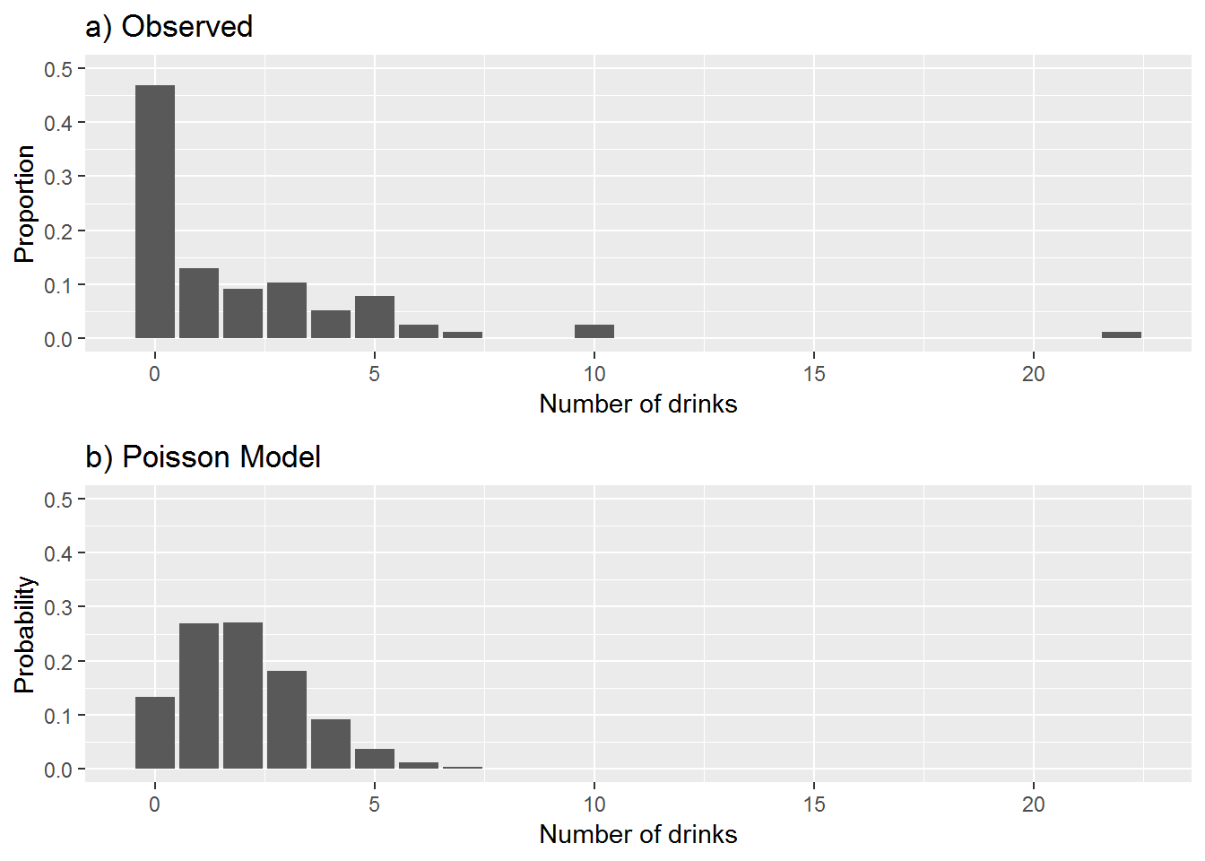
Figure 4.10: Observed (a) versus Modeled (b) Number of Drinks

Beginning the EDA with the response, number of drinks, we find that over 46% of the students reported no drinks during the past weekend. Figure 4.10a portrays the observed number of drinks reported by the students. The mean number of drinks reported the past weekend is 2.013. Our sample consists of 74% females and 26% males, only 9% of whom live off campus.

Because our response is a count it is natural to consider a Poisson regression model. You may recall that a Poisson distribution has only one parameter, \(\lambda\), for its mean and variance. Here we will include an additional parameter, \(\alpha\). We define \(\alpha\) to be the true proportion of non-drinkers in the population.

The next step in the EDA is especially helpful if you suspect your data contains excess zeros. Figure 4.10b is what we might expect to see under a Poisson model. Bars represent the probabilities for a Poisson distribution (using the Poisson probability formula) with \(\lambda\) equal to the mean observed number of drinks, 2.013 drinks per weekend. Comparing this Poisson distribution to what we observed (Figure 4.10a), it is clear that many more zeros have been reported by the students than you would expect to see if the survey observations were coming from a Poisson distribution. This doesn’t surprise us because we had expected a subset of the survey respondents to be non-drinkers; i.e., they would not be included in this Poisson process. This circumstance actually arises in many Poisson regression settings. We will define \(\lambda\) to be the mean number of drinks among those who drink, and \(\alpha\) to be the proportion of non-drinkers (“true zeros”). Then, we will attempt to model \(\lambda\) and \(\alpha\) (or functions of \(\lambda\) and \(\alpha\)) simultaneously using covariates like sex, first-year status, and off-campus residence. This type of model is referred to as a zero-inflated Poisson model or ZIP model.

4.10.4 Modeling

We first fit a simple Poisson model with the covariates off.campus and sex.

glm(formula = drinks ~ off.campus + sex, family = poisson, data = zip.data)

Coefficients:
            Estimate Std. Error z value Pr(>|z|)    
(Intercept)   0.1293     0.1241   1.041    0.298    
off.campus    0.8976     0.2008   4.470 7.83e-06 ***
sexm          1.1154     0.1611   6.925 4.36e-12 ***
---
(Dispersion parameter for poisson family taken to be 1)

    Null deviance: 294.54  on 76  degrees of freedom
Residual deviance: 230.54  on 74  degrees of freedom
AIC: 357.09

# Exponentiated coefficients
exp(coef(pois.m1))

## (Intercept)  off.campus        sexm 
##    1.137996    2.453819    3.050707

# Goodness-of-fit test
gof.ts = pois.m1$deviance
gof.pvalue = 1 - pchisq(gof.ts, pois.m1$df.residual)
gof.pvalue

## [1] 0

Both covariates are statistically significant, but a goodness-of-fit test reveals that there remains significant lack-of-fit (residual deviance: 230.54 with only 74 df; p<.001 based on \(\chi^2\) test with 74 df). In the absence of important missing covariates or extreme observations, this lack-of-fit may be explained by the presence of a group of non-drinkers.

A zero-inflated Poisson regression model to take non-drinkers into account consists of two parts:

• One part models the association, among drinkers, between number of drinks and the predictors of sex and off campus residence.
• The other part uses a predictor for first-year status to obtain an estimate of the proportion of non-drinkers based on the reported zeros.

The form for each part of the model follows. The first part looks like an ordinary Poisson regression model: \[ log(\lambda)=\beta_0+\beta_1(\textrm{off.campus})+ \beta_2(\textrm{sex}) \] where \(\lambda\) is the mean number of drinks in a weekend among those who drink. The second part has the form \[ logit(\alpha)=\beta_0+\beta_1(\textrm{firstYear}) \] where \(\alpha\) is the probability of being in the non-drinkers group and \(logit(\alpha) = log( \alpha/(1-\alpha))\). We’ll provide more detail on the logit in the Logistic Regression chapter. There are many ways in which to structure this model; here we use different predictors in the two pieces, athough it would have been perfectly fine to use the same predictors for both pieces, or even no predictors for one of the pieces.

4.10.5 Fitting a ZIP Model

How is it possible to fit such a model? We cannot observe whether a respondent is a drinker or not (which probably would’ve been good to ask). The ZIP model is a special case of a more general type of statistical model referred to as a latent variable model. More specifically, it is a type of a mixture model where observations for one or more groups occur together and the group membership is unknown. Zero-inflated models are a particularly common example of a mixture model, but the response does not need to follow a Poisson distribution. Likelihood methods are at the core of this methodology, but fitting is an iterative process where it is necessary to start out with some guesses (or starting values). In general, it is important to know that models like ZIP exist, although we’ll only explore interpretations and fitting options for a single case study here.

Here is the general idea of how ZIP models are fit. Imagine that the graph of the Poisson distribution Figure 4.10b is removed from the observed data distribution in Figure 4.10a. Some zero responses will remain. These would correspond to non-drinkers, and the proportion of all observations these zeros constitute might make a reasonable estimate for \(\alpha\), the proportion of non-drinkers. The likelihood is used and some iterating in the fitting process is involved because the Poisson distribution in Figure 4.10b is based on the mean of the observed data, which means it is the average among all students, not only among drinkers. Furthermore, the likelihood incorporates the predictors, sex and off.campus. So there is a little more to it than computing the proportion of zeros, but this heuristic should provide you a general idea of how these kinds of models are fit. The software package R along with the library(pscl) will fit a ZIP model for us using the function zeroinfl.

zeroinfl(formula = drinks ~ off.campus + sex | firstYear, data = zip.data)

Count model coefficients (poisson with log link):
            Estimate Std. Error z value Pr(>|z|)    
(Intercept)   0.7543     0.1440   5.238 1.62e-07 ***
off.campus    0.4159     0.2059   2.021   0.0433 *  
sexm          1.0209     0.1752   5.827 5.63e-09 ***

Zero-inflation model coefficients (binomial with logit link):
              Estimate Std. Error z value Pr(>|z|)  
(Intercept)    -0.6036     0.3114  -1.938   0.0526 .
firstYearTRUE   1.1364     0.6095   1.864   0.0623 .
---
Signif. codes:  0 '***' 0.001 '**' 0.01 '*' 0.05 '.' 0.1 ' ' 1 

exp(coef(zip.m2))   # exponentiated coefficients

##  count_(Intercept)   count_off.campus         count_sexm 
##          2.1260689          1.5157979          2.7756924 
##   zero_(Intercept) zero_firstYearTRUE 
##          0.5468312          3.1154949

Our model uses firstYear to distinguish drinkers and non-drinkers (“Zero-inflation model coefficients”) and off.campus and sex to help explain the differences in the number of drinks among drinkers (“Count model coefficients”). Again, we could have used the same covariates for the two pieces of a ZIP model, but neither off.campus or sex proved to be a useful predictor of drinkers vs. non-drinkers.

We’ll first consider the “Count model coefficients,” which provide information on how the sex and off-campus status of a student who is a drinker are related to the number of drinks reported by that student over a weekend. As we have done with previous Poisson regression models, we exponentiate each coefficient for ease of interpretation. Thus, for those who drink, the average number of drinks for males is \(e^{1.0209}\) or 2.76 times the number for females (Z = 5.827, p < 0.001) given that you are comparing people who live in comparable settings, i.e., either both on or both off campus. Among drinkers, the mean number of drinks for students living off campus is \(e^{0.4159}=1.52\) times that of students living on campus for those of the same sex (Z = 2.021, p = 0.0433).

The “Zero-inflation model coefficients” refer to separating drinkers from non-drinkers. An important consideration in separating drinkers from non-drinkers may be whether this is their first year, where firstYear is a 0/1 indicator variable.

We have \[ log(\alpha/(1-\alpha)) =-0.6036+1.1364(\textrm{firstYear}) \]

However we are interested in \(\alpha\), the proportion of non-drinkers. Exponentiating the coefficient for the first year term for this model yields 3.12. Here it is interpreted as the odds (\(\frac{\alpha}{1-\alpha}\)) that a first year is a non-drinker is 3.12 times the odds that an upper class student is a non-drinker. Furthermore, with a little algebra (solving the equation with \(log(\alpha/(1-\alpha)\)) for \(\alpha\)), we have \[ \hat{\alpha} = \frac{exp^ {-0.6036+1.1364(\textrm{firstYear})}} {1+e^{ -0.6036+1.1364(\textrm{firstYear}) } }. \] The estimated chance that a first year student is a non-drinker is \[ \frac{e^{0.533}}{1+e^{0.533}} = 0.630 \] or 63.0%, while for non-first years, the estimated probability of being a non-drinker in 0.354. If you have seen logistic regression, you’ll recognize that this transformation is what is used to estimate a probability. More on this in the Logistic Regression chapter.

4.10.6 Comparing ZIP to ordinary Poisson with Vuong Test (Optional)

Moving from ordinary Poisson to zero-inflated Poisson has helped us address additional research questions: What proportion of students are non-drinkers and what factors are associated with whether or not a student is a non-drinker? While a ZIP model seems more faithful to the nature and structure of this data, can we quantitatively show that a zero-inflated Poisson is better than an ordinary Poisson model?

We cannot use the drop-in-deviance test we discussed earlier because these two models are not nested within one another. Vuong (1989) devised a test to make this comparison for the special case of comparing a zero-inflated model and ordinary regression model. Essentially, the Vuong Test is able to compare predicted probabilities of non-nested models.

Vuong Non-Nested Hypothesis Test-Statistic: 
(test-statistic is asymptotically distributed N(0,1) under the
 null that the models are indistinguishible)
-------------------------------------------------------------
              Vuong z-statistic             H_A   p-value
Raw                   -2.688691 model2 > model1 0.0035866
AIC-corrected         -2.534095 model2 > model1 0.0056369
BIC-corrected         -2.352922 model2 > model1 0.0093133

Here, we have structured the Vuong Test to compare Model 1: Ordinary Poisson Model to Model 2: Zero-inflation Model. If the two models do not differ, the test statistic for Vuong would be asymptotically standard Normal and the p-value would be relatively large. Here the first line of the output table indicates that the zero-inflation model is better (\(Z=-2.69,p=.0036\)). Note that the test depends upon sufficiently large n for the Normal approximation, so since our sample size (n=77) is somewhat small, we need to interpret this result with caution. More research is underway to address statistical issues related to these comparisons.

4.10.7 Residual Plot

Fitted values (\(\hat{y}\)) and residuals (\(y-\hat{y}\)) can be computed for zero-inflation models and plotted. Figure 4.11 reveals that one observation appears to be extreme (Y=22 drinks during the past weekend). Is this a legitimate observation or was there a transcribing error? Without the original respondents we cannot settle this question. It might be worthwhile to get a sense of how influential this extreme observation is when fitting the model by removing Y=22 and refitting the model.

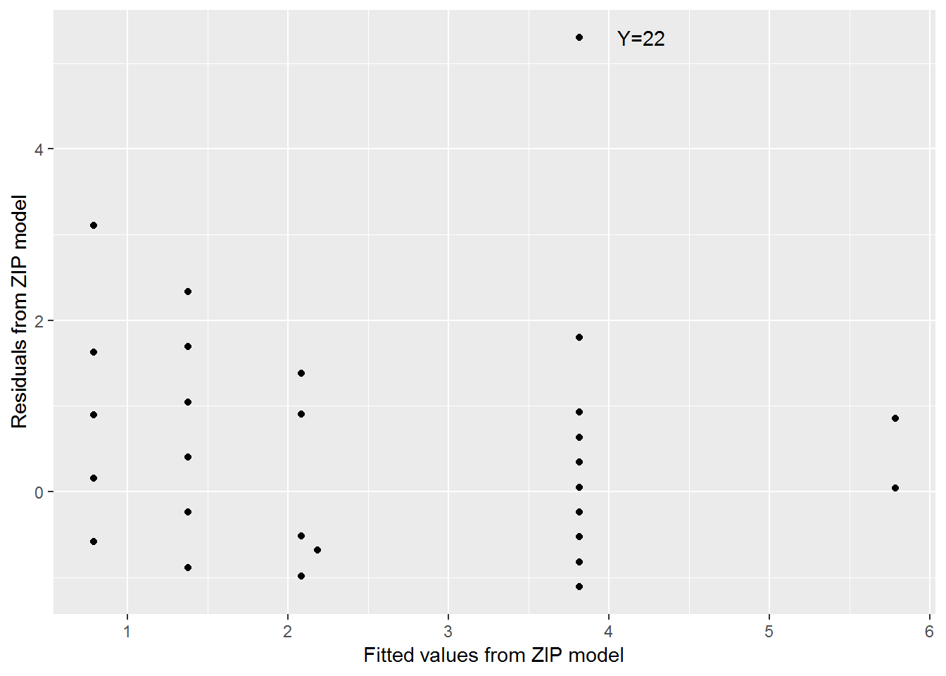
Figure 4.11: Residuals by fitted counts model.

4.10.8 Limitations

Given that you have progressed this far in your statistical education, the weekend drinking survey question should raise some red flags. What time period constitutes the “weekend”? Will some students be thinking of only Saturday night while others include Friday night or possibly Sunday evening? What constitutes a drink—a bottle of beer? How many drinks will a respondent report for a bottle of wine? Precise definitions would vastly improve the quality of this data. There is also an issue related to confidentiality. If the data is collected in class, will the teacher be able to identify the respondent? Will respondents worry that a particular response will affect their grade in the class or lead to repercussions on a dry campus?

In addition to these concerns, there are a number of other limitations that should be noted. Following the concern of whether this data represents a random sample of any population (it doesn’t), we also must be concerned with the size of this data set. ZIP models are not appropriate for small samples and this data set is not impressively large.

At times, a mixture of zeros occurs naturally. It may not come about because of neglecting to ask a critical question on a survey, but the information about the subpopulation may simply not be ascertainable. For example, visitors from a state park were asked as they departed how many fish they caught, but those who report 0 could be either non-fishers or fishers who had bad luck. These kinds of circumstances occur often enough that ZIP models are becoming increasingly common.

Actually there are many fewer ordinary Poisson regression applications in contrast to ZIPs and other Poisson modeling approaches such as hurdle models and quasi-Poisson applications. So it is worth taking a look at these variations of Poisson regression models. Not enough detail is presented here to deal with certain nuances of zero-inflated models, but we want you to know about models of this type. ZIP models demonstrate that modeling can be flexible and creative which we hope you see as a theme throughout this book.

4.11 Exercises

4.11.1 Conceptual Exercises

Each example 1-4 involves predicting a response using one or more explanatory variables, where these examples have response variables that are counts per some unit of time or space. List the response (both what is being counted and over what unit of time or space) and relevant explanatory variables.

1. Are the number of motorcycle deaths in a given year related to a state’s helmet laws?
2. Does the number of employers conducting on-campus interviews during a year differ for public and private colleges?
3. Does the daily number of asthma-related visits to an Emergency Room differ depending on air pollution indices?

4. Has the number of deformed fish in randomly selected Minnesota lakes been affected by changes in trace minerals in the water over the last decade?

5. Models of the form \(Y_i=\beta_0+\beta_1X_i+\epsilon_i, \epsilon_i \sim iidN(0,\sigma)\) are fit using the method of least squares. What method is used to fit Poisson regression models?
6. What should be done before adjusting for overdispersion?
7. Why is quasilikelihood used and how do the results compare for corresponding models using likelihoods?
8. Why is the log of mean counts, log(\(\bar{Y}\)), not \(\bar{Y}\), plotted against X when assessing the assumptions for Poisson regression?
9. How can this assumption of mean=variance be checked for Poisson regression? What if there are not many repeated observations at each level of X?

10. Is it possible that a predictor is significant for a model fit using a likelihood, but not for a model for the same data fit using a quasilikelihood? Explain.

Complete (a)-(d) in the context of the study for Exercises 11-13.

1. Define the response.
2. What are the possible values for the response?
   
3. What does \(\lambda\) represent?
4. Would a zero-inflated model be considered here? If so, what would be a “true zero?”

11. Fish (Poisson) A state wildlife biologist collected data from 250 park visitors as they left at the end of their stay. Each was asked to report the number of fish they caught during their one week stay. On average visitors caught 21.5 fish per week.

12. Methadone Program Recidivism. Program facilitators keep track of the number of times their program’s patients relapse within five years of initial treatment. Data on 100 patients yielded a mean number of 2.8 relapses per patient within the five years of initial treatment.

13. Clutch size. Thirty nests were located and the number of eggs in each nest were counted at the start of a season. Later in the season following a particularly destructive storm, the mean clutch size of the 30 nests was only 1.7 eggs per nest.

14. Credit card use A survey of 1,000 consumers asked respondents how many credit cards they use. Interest centers on the relationship between credit card use and income, in $10,000. The estimated coefficient for income is 2.1.

    • Identify the predictor and interpret the estimated coefficient for the predictor in this context.
    • Describe how the assumption of linearity can be assessed in this example.
    • Suggest a way in which to assess the equal mean and variance assumption.

15. Dating Online Researchers are interested in the number of dates respondents arranged online and whether the rates differ by age group. Questions which elicit responses similar to this can be found in the Pew survey concerning dating online and relationships (Smith and Duggan 2013). Each survey respondent was asked how many dates they have arranged online in the past 3 months as well as the typical amount of time, \(t\), in hours, they spend online weekly. Some rows of data appear below.

Age	Time online	Number of dates arranged online
19	35	3
29	20	5
38	15	0
55	10	0

• Identify the response, predictor, and offset in this context. Does using an offset make sense?
• Write out a model for this data. As part of your model description, define the parameter, \(\lambda\).
• Consider a Zero-inflated Poisson model for this data. Describe what the `true zeros’ would be in this setting.

16. Poisson Approximation: Rare Events For rare diseases, the probability of a case occurring, \(p\), in a very large population, \(n\), is small. With a small \(p\) and large \(n\), the random variable \(Y\)= the number of cases out of \(n\) people can be approximated using a Poisson random variable with \(\lambda = np\). If the count of those with the disease is observed in several different populations independently of one another, the \(Y_i\) represents the number of cases in the \(i^{th}\) population and can be approximated using a Poisson random variable with \(\lambda_i=n_ip_i\) where \(p_i\) is the probability of a case for the \(i^{th}\) population. Poisson regression can take into account the differences in the population sizes, \(n_i\), using as an offset which is log(\(n_i\)). The coefficient of the offset is set at one; it is not estimated like the other coefficients. Thus the model statement has the form: \[ log(\lambda_i) = \beta_0+\beta_1x_i + log(n_i) \] where \(Y_i \sim\) Poisson(\(\lambda_i = n_i p_i\)). Note that \(\lambda_i\) depends on \(x_i\) which may differ for the different populations.

Data from Scotto, Kopf, and Urbach (1974) reported the number of cases of non melanoma skin cancer for women by age group in two metropolitan areas (Minneapolis-St Paul and Dallas-Ft Worth); the year is unknown. They wondered if cancer rates by age group differ by city? The columns contain: number of cases of skin cancer, population size of the age group per city, age group, and metropolitan area (1=Minneapolis-St Paul, 2=Dallas-Ft Worth).

Number of Cases	Population	Age Group	City
1	172675	15-24	1
16	123065	25-34	1
…	…	…	…
226	29007	75-84	2
65	7538	85+	2

Identify and describe the following quantities which appear in the description of the Poisson approximation for rare events:

• A case,
• The population size, \(n_i\),
• Probability, \(p_i\),
• Poisson parameter, \(\lambda_i\),
• Poisson random variables, \(Y_i\), and
• The predictors, \(X_i\).

4.11.2 Guided Exercise

1. We wish to build a regression model to describe the number of burglaries on a college campus in a year. Our population of interest will be U.S. liberal arts colleges.

1. Describe why the response variable (\(Y\) = # burglaries on campus in a year) could be modeled by a Poisson distribution.
2. Describe explanatory variables which might explain differences in \(\lambda\) = mean number of burglaries per year on a particular campus.
3. Consider a campus with an average of 5 burglaries per year. Use dpois() to sketch a plot of the distribution of \(Y\) for this campus. Use rpois() to verify that both the mean and variance of \(Y\) are given by \(\lambda=5\).
4. Consider a campus with an average of 20 burglaries per year and repeat (c).

2. Elephant Mating How does age affect male elephant mating patterns? An article by Poole (1989) investigated whether mating success in male elephants increases with age and whether there is a peak age for mating success. To address this question, the research team followed 41 elephants for one year and recorded both their ages and their number of matings. The data is found in elephant.csv, and the variables are:

• MATINGS = the number of matings in a given year
• AGE = the age of the elephant in years.

1. Create a histogram of MATINGS. Is there preliminary evidence that number of matings could be modeled as a Poisson response? Explain.
2. Plot MATINGS by AGE. Add a least squares line. Is there evidence that modeling matings using a linear regression with age might not be appropriate? Explain. (Hints: fit a smoother; check residual plots)
3. For each age, calculate the mean number of matings. Take the log of each mean and plot it by AGE.
   1. What assumption can be assessed with this plot?
   2. Is there evidence of a quadratic trend on this plot?
4. Fit a Poisson regression model with a linear term for AGE. Exponentiate and then interpret the coefficient for AGE.
5. Construct a 95% confidence interval for the slope and interpret in context (you may want to exponentiate endpoints).
6. Are the number of matings significantly related to age? Test with
   1. a Wald test and
   2. a drop in deviance test.
7. Add a quadratic term in AGE to determine whether there is a maximum age for the number of matings for elephants. Is a quadratic model preferred to a linear model? To investigate this question, use
   1. a Wald test and
   2. a drop in deviance test.
8. What can we say about the goodness of fit of the model with age as the sole predictor? Compare the residual deviance for the linear model to a \(\chi^2\) distribution with the residual model degrees of freedom.
9. Fit the linear model using a quasilikelihood. (Why?)
   1. How do the estimated coefficients change?
   2. How do the standard errors change?
   3. What is the estimated dispersion parameter?
   4. An estimated dispersion parameter greater than one suggests overdispersion. When adjusting for overdispersion, are you more or less likely to obtain a significant result when testing coefficients? Why?

Source: (Ramsey and Schafer 2002).

3. Smoking at Work and Home An earlier study examined the effect of workplace rules in Minnesota which require smokers to smoke cigarettes outside. The number of cigarettes smoked by smokers in a 2-hour period was recorded, along with whether the smoker was at home or at work. A (very) small subset of the data appears below:

Table 4.5: A small subset of hypothetical data on Minnesota workplace rules on smoking. X is 0 for home and 1 for work. Y is number of cigaretttes in a 2-hour period.

Subject	X (location)	Y (cigarettes)
1	0	3
2	1	0
3	1	0
4	1	1
5	0	2
6	0	1

• Model 1: Assume that \(Y \sim \textrm{Poisson}(\lambda)\); there is no difference between home and work.
• Model 2: Assume that \(Y \sim \textrm{Poisson}(\lambda_W)\) when the smoker is at work, and \(Y \sim \textrm{Poisson}(\lambda_H)\) when the smoker is at home.
• Model 3: Assume that \(Y \sim \textrm{Poisson}(\lambda)\) and \(log(\lambda)=\beta_0+\beta_1X\).

1. Write out the likelihood \(L(\lambda)\) and the log-likelihood \(logL(\lambda)\) in Model 1. Use the data values above, and simplify where possible.
2. Intuitively, what would be a reasonable estimate for \(\lambda\) based on this data? Why?
3. Find the maximum likelihood estimator for \(\lambda\) in Model 1 using an optimization routine in R (but not the glm() function). Use R to produce a plot of the likelihood function \(L(\lambda)\).
4. Write out the log-likelihood function \(logL(\lambda_W, \lambda_H)\) in Model 2. Use the data values above, and simplify where possible.
5. Intuitively, what would be reasonable estimates for \(\lambda_W\) and \(\lambda_H\) based on this data? Why?
6. Find the maximum likelihood estimators for \(\lambda_W\) and \(\lambda_H\) in Model 2 using an optimization routine in R (but not the glm() function).

4. Smoking at Work and Home (continued) We will use the same dataset in this question as we used in question 3.

1. Write out the log-likelihood function \(logL(\beta_0, \beta_1)\) in Model 3. Again, use the data values above, and simplify where possible.
2. Find the maximum likelihood estimators for \(\beta_0\) and \(\beta_1\) in Model 3 using an optimization routine in R (but not the glm() function). Use R to produce a 3D plot of the log-likelihood function.
3. Confirm your estimates for Model 1 and Model 3 using glm(). Then show that the MLEs for Model 3 agree with the MLEs for Model 2.

For the remaining questions, we will focus exclusively on Model 3.

4. State a (one-sided) hypothesis for \(\beta_1\) in the context of the problem (i.e. explain how your hypothesis relates to smoking at home and at work). Note: we will nevertheless use two-sided tests and intervals in the following questions.
5. Do we need to include an offset in our Poisson regression model? Why or why not?
6. Give estimates of \(\beta_0\) and \(\beta_1\), and provide interpretations for both in the context of the problem.
7. Provide and interpret a 95% confidence interval for \(\beta_1\).
8. Provide two different significance tests for \(\beta_1\), in each case providing a test statistic and a p-value and a conclusion in the context of the problem.
9. Provide a goodness-of-fit test for Model 3, again providing a test statistic, p-value, and conclusion in context.
10. Can we generalize results of this study to all Minnesota smokers? Why or why not.
11. Can we claim that rules restricting smoking in the workplace have caused lower levels of smoking at work? Explain.
12. Give two ways in which this study might be improved (besides simply “bigger sample size”).

5. Campus Crime The data set campuscrime09.csv contains the number of burglaries reported at a collection of 47 US public universities with over 10,000 students in the year 2009. In addition, covariates are included which may explain differences in crime rates, including total number of students, percentage of men, average SAT and ACT test scores, and tuition.

1. Perform an exploratory data analysis. Support your analysis with plots and summary statistics.
   1. Analyze whether number of burglaries could be reasonably modeled with a Poisson distribution
   2. Analyze which covariates you expect to be the best predictors of burglaries.
      
2. Consider a model with 4 predictors: act.comp + tuition + pct.male + total. Try fitting a linear regression with burg09 as the response. Are there any concerns with this linear regression model?
3. Run a Poisson regression model with the 4 predictors from (b). Interpret the coefficients for tuition and pct.male.
4. Replace tuition with tuition in thousands in your model from (c) – i.e. tuition.thous=tuition/1000. How does your new model compare to your model in (c)? Interpret the coefficient for tuition.thous.
5. We will consider the possibility of including the total number of students at a university as an offset.
   1. Explain why we might consider total as an offset.
   2. Refit your model from (d) with total (actually, log(total)) as an offset rather than as a predictor. Does this new model appear to fit better or worse than the model from (d)?
   3. Refit your model from (d) with log(total) rather than total – so log(total) is a predictor and not an offset. If total were a good candidate for an offset, what would we expect the coefficient of log(total) to be? Does a 95% confidence interval for that coefficient contain the value you expected?
6. Run the following model, then interpret the coefficients for tuition.thous and the interaction between tuition.thous and act.comp.

crime <- mutate(crime, total.thous = total/1000)
fit3 <- glm(burg09 ~ act.comp + tuition.thous + total.thous +
  act.comp:tuition.thous + act.comp:total.thous, family = poisson, data = crime)

6. US National Medical Expenditure Survey The data set NMES1988 in the AER package contains a sample of individuals over 65 who are covered by Medicare in order to assess the demand for health care through physician office visits, outpatient visits, ER visits, hospital stays, etc. The data can be accessed by installing the AER package and then running:

library(AER)
data(NMES1988)

More background information and references about the NMES1988 data can be found in help pages for the AER package.

1. Show through graphical means that there are more respondents with 0 visits than might be expected under a Poisson model.
2. Fit a model for the number of physician office visits using chronic, health, and insurance as predictors for the Poisson count, and chronic and insurance as the predictors for the binary part of the model. Then, provide interpretations in context for the following model parameters:

• chronic in the Poisson part of the model
• poor health in the Poisson part of the model
• the Intercept in the logistic part of the model
• insurance in the logistic part of the model

3. Is there significant evidence that the ZIP model is an improvement over a simple Poisson regression model?

7. Going Vague: Ambiguity in Political Issue Statements In the following exercise, you will use a hurdle model to analyze the data. A hurdle model is similar to a zero-inflated poisson model, but instead of assuming that “zeros” are comprised of two distinct groups—those who would always be 0 and those who happen to be 0 on this occasion (e.g. non-drinkers and drinkers who had zero drinks over the weekend in Case Study 4.10)—the hurdle model assumes that “zeros” are a single entity. Therefore, in a hurdle model, cases are classified as either “zeros” or “non-zeros”, where “non-zeros” hurdle the 0 threshold—they must always have counts of 1 or above. We will use the pscl package and the hurdle function in it, to analyze a hurdle model. Note that coefficients in the “zero hurdle model” section of the output relate predictors to the log-odds of being a non-zero (i.e., having at least one issue statement).

In a 2018 study, Chapp et al. (2018) scraped every issue statement from webpages of candidates for the US House of Representatives, counting the number of issues candidates commented on and scoring the level of ambiguity of each statement. We will focus on the issue counts, and determining which attributes (of both the district as a whole and the candidates themselves) are associated with candidate silence (commenting on 0 issues) and a willingness to comment on a greater number of issues. The data set ambiguity.csv contains the following variables:

• name : candidate name
• distID : unique identification number for Congressional district
• ideology : candidate left-right orientation
• democrat : 1 if Democrat, 0 if Republican
• mismatch : disagreement between candidate ideology and district voter ideology
• incumbent : 1 if incumbent, 0 if not
• demHeterogeneity : how much voters in a district differ according to race, education, occupation, etc.
• attHeterogeneity : how much voters in a district differ according to political ideology
• distLean : overall ideological lean in a district
• totalIssuePages : number of issues candidates commented on (response)

1. Create a frequency plot of total_issue_pages. Why might we consider using a hurdle model compared to a poisson model? Why can’t we use a zero-inflated poisson model?
2. Create a plot of the empirical log odds of having at least one issue statement by ideology. You may want to group ideology values first. What can you conclude from this plot?
3. Create a scatter plot that shows the log of the mean number of issues vs ideology group by party, among candidates with at least one issue statement. What can we conclude from this plot?
4. Create a hurdle model with ideology and democrat as predictors in both parts. Interpret ideology in both parts of the model.
5. Repeat (d), but include an interaction in both parts. Interpret the interaction in the zero hurdle part of the model.
6. Find the best model you can to determine total_issue_pages. Write a short paragraph discussing implications of your model.

4.11.3 Open-ended

1. Airbnb in NYC. Airbnb is an online service that allows travelers to book a stay with only a few clicks at any given time. Customers are given the ability to tailor their travel experience to fit their budget and lifestyle, choosing from castles to tree houses, and finding plenty of offerings in rural towns as well as busy metropolitan areas. In a break from traditional industrial models, Airbnb promotes the growth of a “sharing economy,” a way to supplement income by renting out or otherwise utilizing existing assets for individual profit. There are few barriers to entry to become a seller on the rental market for Airbnb, and its global reach provides an instantaneous way to make money for its wide user base.

Awad, Lebo, and Linden (2017) scraped 40628 Airbnb listings from New York City in March 2017 and put together the data set NYCairbnb.csv. Key variables include:

• id = unique ID number for each unit
• last_scraped = date when information scraped
• host_since = date when host first listed the unit on Airbnb
• days = last_scraped - host_since = number of days the unit has been listed
• room_type = Entire home/apt, Private room, or Shared room
• bathrooms = number of bathrooms
• bedrooms = number of bedrooms
• price = price per night (dollars)
• number_of_reviews = number of reviews for the unit on Airbnb
• review_scores_cleanliness = cleanliness score from reviews (1-10)
• review_scores_location = location score from reviews (1-10)
• review_scores_value = value score from reviews (1-10)
• instant_bookable = “t” if instantly bookable, “f” if not

Perform an EDA, build a model, and interpret model coefficients to describe variation in the number of reviews (a proxy for the number of rentals, which is not available) as a function of the variables provided. Don’t forget to consider an offset, if needed.

2. Crab Satellites

Brockmann (1996) carried out a study of nesting female horseshoe crabs. Female horseshoe crabs often have male crabs attached to a female’s nest known as satellites. One objective of the study was to determine which characteristics of the female were associated with the number of satellites. Of particular interest is the relationship between the width of the female carapace and satellites. The data can be found in crab.csv. It includes:

• NumSat = number of satellites
• Width = carapace width (cm)
• Wt = weight (kg)
• Sp = spine condition (1 = both good, 2 = one worn or broken, 3 = both worn or broken)
• C = color (1 = light medium, 2 = medium, 3 = dark medium, 4 = dark)

Use Poisson regression to investigate the research question. Be sure you work to obtain an appropriate model before considering overdispersion.

3. Doctor Visits

Data was collected on doctor visits from a sample of 5,190 people in the 1977/1978 Australian Health Survey. Cameron and Trivedi (1986) sought to explain the variation in doctor visits using one or more explanatory variables. The data can be found in an R data set from library(AER) accessible with the command data("DoctorVisits"). Variable descriptions can be found under help("DoctorVisits")

Explore the use of a zero-inflated model for this data. Begin with a histogram of the number of visits, some EDA, and fitting several models. Summarize your results.

4. More Fish

The number of fish caught (count), persons in the party (persons), the number of children in the party (child), whether or not they brought a camper into the park (camper), and the length of stay (LOS) were recorded for 250 camping parties. The data can be found in fish2.csv (source: (“Zero-Inflated Negative Binomial Regression | R Data Analysis Examples” 2018)). Create and assess a model for the number of fish caught.

References

Philippine Statistics Authority. 2015. “Family Income and Expenditure Survey.” https://www.kaggle.com/grosvenpaul/family-income-and-expenditure.

McCullagh, Peter, and John Ashworth Nelder. 1989. Generalized Linear Models. Second Edition. Boca Raton, Florida: Chapman; Hall/ CRC Monographs on Statistics; Applied Probability.

Smith, Aaron, and Maeve Duggan. 2013. “Online Dating and Relationships.” Pew Research Center: Internet and Technology.

Scotto, Joseph, Alfred W. Kopf, and Fredrick Urbach. 1974. “Non-Melanoma Skin Cancer Among Caucasians in Four Areas of the United States.” Cancer 34 (4): 1333–8. doi:10.1002/1097-0142(197410)34:4<1333::AID-CNCR2820340447>3.0.CO;2-A.

Poole, Joyce H. 1989. “Mate Guarding, Reproductive Success and Female Choice in African Elephants.” Animal Behaviour 37: 842–49. doi:https://doi.org/10.1016/0003-3472(89)90068-7.

Ramsey, Fred, and Daniel Schafer. 2002. The Statistical Sleuth: A Course in Methods of Data Analysis. Second Edition. Boston, Massachusetts: Brooks/ Cole Cengage Learning.

Chapp, Christopher, Paul Roback, Kendra Jo Johnson-Tesch, Adrian Rossing, and Jack Werner. 2018. “Going Vague: Ambiguity and Avoidance in Online Political Messaging.” Social Science Computer Review.

Awad, Annika, Evan Lebo, and Anna Linden. 2017. “Intercontinental Comparative Analysis of Airbnb Booking Factors.” Project for Statistics 316-Advanced Statistical Modeling, St. Olaf College.

Brockmann, H. Jane. 1996. “Satellite Male Groups in Horseshoe Crabs, Limulus Polyphemus.” Ethology 102 (1): 1–21. doi:doi:10.1111/j.1439-0310.1996.tb01099.x.

Cameron, A.C., and P.K. Trivedi. 1986. “Econometric Models Based on Count Data: Comparisons and Applications of Some Estimators and Tests.” Journal of Applied Econometrics 1: 29–53.

“Zero-Inflated Negative Binomial Regression | R Data Analysis Examples.” 2018. https://stats.idre.ucla.edu/r/dae/zinb/.