Chapter 6 Logistic Regression

\[ \newcommand{\lik}{\operatorname{Lik}} \newcommand{\Lik}{\operatorname{Lik}} \]

6.1 Learning Objectives

• Identify a binomial random variable and assess the validity of the binomial assumptions.
• Write a generalized linear model for binomial responses in two forms, one as a function of the logit and one as a function of \(p\).
• Explain how fitting a logistic regression differs from fitting an ordinary least squares (OLS) regression model.
• Interpret estimated coefficients in logistic regression.
• Differentiate between logistic regression models with binary and binomial responses.
• Use the residual deviance to compare models, to test for lack-of-fit when appropriate, and to check for unusual observations or needed transformations.

6.2 Introduction to Logistic Regression

Logistic regression is characterized by research questions with binary (yes/no or success/failure) or binomial (number of yesses or successes in \(n\) trials) responses:

• 1. Are students with poor grades more likely to binge drink?
• 2. Is exposure to a particular chemical associated with a cancer diagnosis?
• 3. Are the number of votes for a congressional candidate associated with the amount of campaign contributions?

Binary Responses: Recall from Section 3.3.1 that binary responses take on only two values: success (Y=1) or failure (Y=0), Yes (Y=1) or No (Y=0), etc. Binary responses are ubiquitous; they are one of the most common types of data that statisticians encounter. We are often interested in modeling the probability of success \(p\) based on a set of covariates, although sometimes we wish to use those covariates to classify a future observation as a success or a failure.

Examples (a) and (b) above would be considered to have binary responses (Does a student binge drink? Was a patient diagnosed with cancer?), assuming that we have a unique set of covariates for each individual student or patient.

Binomial Responses: Also recall from Section 3.3.2 that binomial responses are number of successes in \(n\) identical, independent trials with constant probability \(p\) of success. A sequence of independent trials like this with the same probability of success is called a Bernoulli process. As with binary responses, our objective in modeling binomial responses is to quantify how the probability of success, \(p\), is associated with relevant covariates.

Example (c) above would be considered to have a binonial response, assuming we have vote totals at the congressional district level rather than information on individual voters.

6.2.1 Logistic Regression Assumptions

Much like OLS, using logistic regression to make inferences requires model assumptions.

1. Binary Response The response variable is dichotomous (two possible responses) or the sum of dichotomous responses.
2. Independence The observations must be independent of one another.
3. Variance Structure By definition, the variance of a binomial random variable is \(np(1-p)\), so that variability is highest when \(p=.5\).
4. Linearity The log of the odds ratio, log(\(\frac{p}{1-p}\)), must be a linear function of x. This will be explained further in the context of the first case study.

6.2.2 A Graphical Look at Logistic Regression

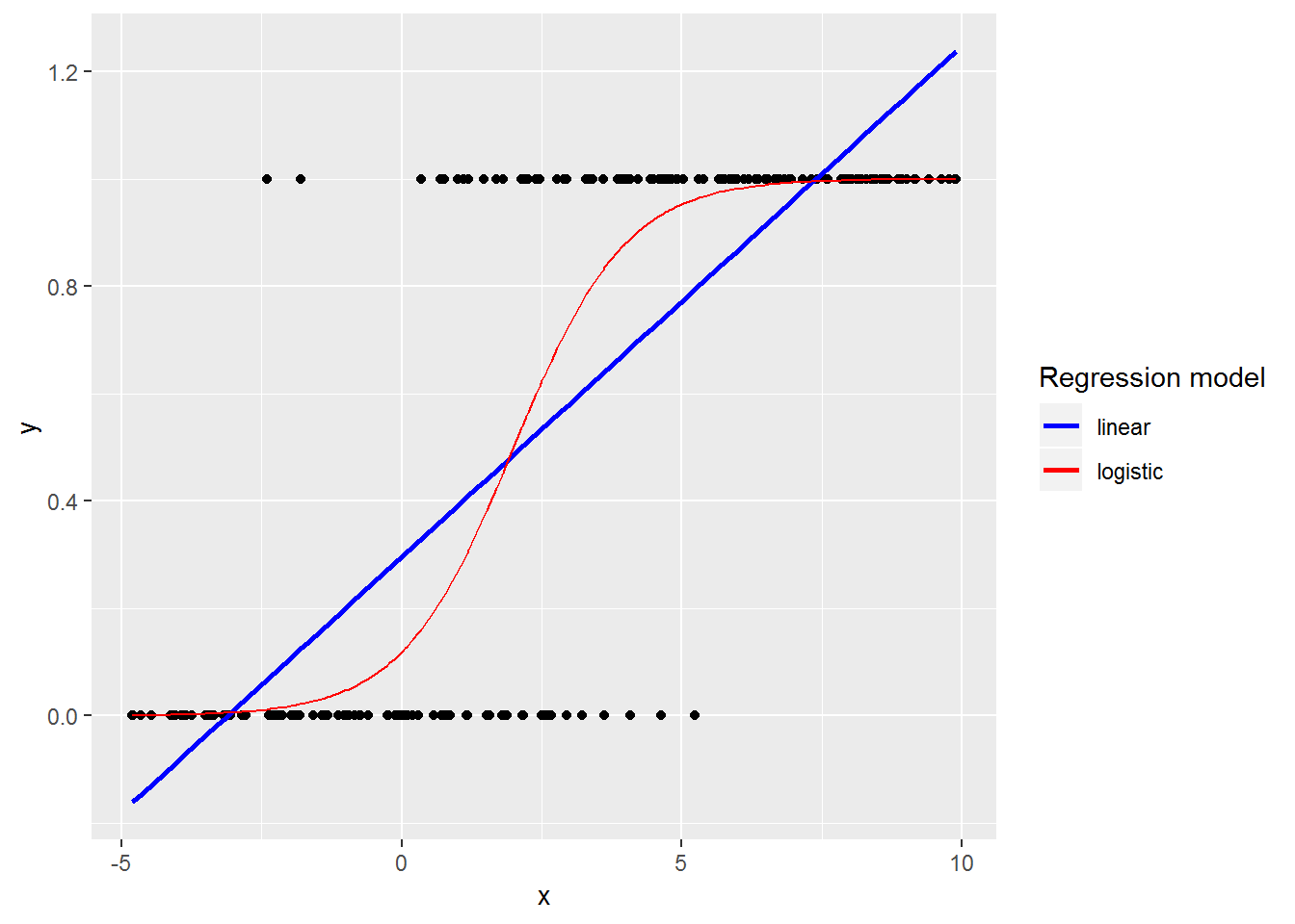
Figure 6.1: Linear vs. Logistic regression models for binary response data.

Figure 6.1 illustrates a data set with a binary (0 or 1) response (Y) and a single continuous predictor (X). The blue line is a linear regression fit with OLS to model the probability of a success (Y=1) for a given value of X. With a binary response, the line doesn’t fit the data well, and it produces predicted probabilities below 0 and above 1. On the other hand, the logistic regression fit (red curve) with its typical “S” shape follows the data closely and always produces predicted probabilities between 0 and 1. For these and several other reasons detailed in this chapter, we will focus on the following model for logistic regression with binary or binomial responses:

\[\begin{equation} log(\frac{p_i}{1-p_i})=\beta_0+\beta_1 x_i \tag{6.1} \end{equation}\]

where the observed values \(Y_i \sim\) binomial with \(p=p_i\) for a given \(x_i\) and \(n=1\) for binary responses.

6.3 Case Studies Overview

We consider three case studies in this chapter. The first two involve binomial responses (Soccer Goalkeepers and Reconstructing Alabama), while the last case uses a binary response (Trying to Lose Weight). Even though binary responses are much more common, their models have a very similar form to binomial responses, so the first two case studies will illustrate important principles that also apply to the binary case. Here are the statistical concepts you will encounter for each Case Study.

The soccer goalkeeper data can be written in the form of a 2 \(\times\) 2 table. This example is used to describe some of the underlying theory for logistic regression. We demonstrate how binomial probability mass functions (pmfs) can be written in one parameter exponential family form, from which we can identify the canonical link as in Chapter 5. Using the canonical link, we write a Generalized Linear Model for binomial counts and determine corresponding MLEs for model coefficients. Interpretation of the estimated parameters involves a fundamental concept, the odds ratio.

The Reconstructing Alabama case study is another binomial example which introduces the notion of deviances, which are used to compare and assess models. We will check the assumptions of logistic regression using empirical logit plots and deviance residuals.

The last case study addresses why teens try to lose weight. Here the response is a binary variable which allows us to analyze individual level data. The analysis builds on concepts from the previous sections in the context of a random sample from CDC’s Youth Risk Behavior Survey (YRBS).

6.4 Case Study: Soccer Goalkeepers

Does the probability of a save in a soccer match depend upon whether the goalkeeper’s team is behind or not? Roskes et al. (2011) looked at penalty kicks in the men’s World Cup soccer championships from 1982 - 2010, and they assembled data on 204 penalty kicks during shootouts. The data for this study is summarized in Table 6.1.

Table 6.1: Soccer goalkeepers’ saves when their team is and is not behind. Source: Roskes et al. 2011 Psychological Science

	Saves	Scores	Total
Behind	2	22	24
Not Behind	39	141	180
Total	41	163	204

6.4.1 Modeling Odds

Odds are one way to quantify a goalkeeper’s performance. Here the odds that a goalkeeper makes a save when his team is behind is 2 to 22 or 0.09 to 1. Or equivalently, the odds that a goal is scored on a penalty kick is 22 to 2 or 11 to 1. An odds of 11 to 1 tells you that a shooter whose team is ahead will score 11 times for every 1 shot that the goalkeeper saves. When the goalkeeper’s team is not behind the odds a goal is scored is 141 to 39 or 3.61 to 1. We see that the odds of a goal scored on a penalty kick are better when the goalkeeper’s team is behind than when it is not behind (i.e., better odds of scoring for the shooter when the shooter’s team is ahead). We can compare these odds by calculating the odds ratio (OR), 11/3.61 or 3.05, which tells us that the odds of a successful penalty kick are 3.05 times higher when the shooter’s team is leading.

In our example, it is also possible to estimate the probability of a goal, \(p\), for either circumstance. When the goalkeeper’s team is behind, the probability of a successful penalty kick is \(p\) = 22/24 or 0.833. We can see that the ratio of the probability of a goal scored divided by the probability of no goal is \((22/24)/(2/24)=22/2\) or 11, the odds we had calculated above. The same calculation can be made when the goalkeeper’s team is not behind. In general, we now have several ways of finding the odds of success under certain circumstances: \[\textrm{Odds} = \frac{\# \textrm{successes}}{\# \textrm{failures}}= \frac{\# \textrm{successes}/n}{\# \textrm{failures}/n}= \frac{p}{1-p}.\]

6.4.2 Logistic Regression Models for Binomial Responses

We would like to model the odds of success, however odds are strictly positive. Therefore, similar to modeling log(\(\lambda\)) in Poisson regression, which allowed the response to take on values from \(-\infty\) to \(\infty\), we will model the log(odds), the logit, in logistic regression. Logits will be suitable for modeling with a linear function of the predictors:
\[\begin{equation} \log\left(\frac{p}{1 - p}\right)=\beta_0+\beta_1X \tag{6.2} \end{equation}\]

Models of this form are referred to as binomial regression models, or more generally as logistic regression models. Here we provide intuition for using and interpreting logistic regression models, and then in the short optional section that follows, we present rationale for these models using GLM theory.

In our example we could define \(X=0\) for not behind and \(X=1\) for behind and fit the model: \[\begin{equation} \log\left(\frac{p_X}{1-p_X}\right)=\beta_0 +\beta_1X \tag{6.3} \end{equation}\]

where \(p_X\) is the probability of a successful penalty kick given \(X\).

So, based on this model, the log odds of a successful penalty kick when the goalkeeper’s team is not behind is: \[ \log\left(\frac{p_0}{1-p_0}\right) =\beta_0 \nonumber, \] and the log odds when the team is behind is: \[ \log\left(\frac{p_1}{1-p_1}\right)=\beta_0+\beta_1. \nonumber \]

We can see that \(\beta_1\) is the difference between the log odds of a successful penalty kick between games when the goalkeeper’s team is behind and games when the team is not behind. Using rules of logs: \[\begin{equation} \beta_1 = (\beta_0 + \beta_1) - \beta_0 = \log\left(\frac{p_1}{1-p_1}\right) - \log\left(\frac{p_0}{1-p_0}\right) = \log\left(\frac{p_1/(1-p_1)}{p_0/{(1-p_0)}}\right). \tag{6.4} \end{equation}\]

Thus \(e^{\beta_1}\) is the ratio of the odds of scoring when the goalkeeper’s team is not behind compared to scoring when the team is behind. In general, exponentiated coefficients in logistic regression are odds ratios (OR). A general interpretation of an OR is the odds of success for group A compared to the odds of success for group B—how many times greater the odds of success are in group A compared to group B.

The logit model (Equation (6.3)) can also be re-written in a probability form: \[\begin{equation} p_X=\frac{e^{\beta_0+\beta_1X}}{1+e^{\beta_0+\beta_1X}} \tag{6.5} \end{equation}\] which can be re-written for games when the goalkeeper’s team is behind as: \[\begin{equation} p_1=\frac{e^{\beta_0+\beta_1}}{1+e^{\beta_0+\beta_1}} \tag{6.6} \end{equation}\] and for games when the goalkeeper’s team is not behind as: \[\begin{equation} p_0=\frac{e^{\beta_0}}{1+e^{\beta_0}} \tag{6.7} \end{equation}\]

We use likelihood methods to estimate \(\beta_0\) and \(\beta_1\). As we had done in Chapter 2, we can write the likelihood for this example in the following form: \[\Lik(p_1, p_0) = {28 \choose 22}p_1^{22}(1-p_1)^{2} {180 \choose 141}p_0^{141}(1-p_0)^{39}\]

Our interest centers on estimating \(\hat{\beta_0}\) and \(\hat{\beta_1}\), not \(p_1\) or \(p_0\). So we replace \(p_1\) in the likelihood with an expression for \(p_1\) in terms of \(\beta_0\) and \(\beta_1\) as in Equation (6.6). Similarly, \(p_0\) in Equation (6.7) involves only \(\beta_0\). After removing constants, the new likelihood looks like:

\[\begin{equation} \Lik(\beta_0,\beta_1) \propto \left( \frac{e^{\beta_0+\beta_1}}{1+e^{\beta_0+\beta_1}}\right)^{22}\left(1- \frac{e^{\beta_0+\beta_1}}{1+e^{\beta_0+\beta_1}}\right)^{2} \left(\frac{e^{\beta_0}}{1+e^{\beta_0}}\right)^{141}\left(1-\frac{e^{\beta_0}}{1+e^{\beta_0}}\right)^{39} \tag{6.8} \end{equation}\]

Now what? Fitting the model means finding estimates of \(\beta_0\) and \(\beta_1\), but familiar methods from calculus for maximizing the likelihood don’t work here. Instead, we consider all possible combinations of \(\beta_0\) and \(\beta_1\). That is, we will pick that pair of values for \(\beta_0\) and \(\beta_1\) that yield the largest likelihood for our data. Trial and error to find the best pair is tedious at best, but more efficient numerical methods are available. The MLEs for the coefficients in the soccer goalkeeper study are \(\hat{\beta_0}= 1.2852\) and \(\hat{\beta_1}=1.1127\).

Exponentiating \(\hat{\beta_1}\) provides an estimate of the odds ratio (the odds of scoring when the goalkeeper’s team is behind compared to the odds of scoring when the team is not behind) of 3.04, which is consistent with our calculations using the 2 \(\times\) 2 table. We estimate that the odds of scoring when the goalkeeper’s team is behind is over 3 times that of when the team is not behind or, in other words, the odds a shooter is successful in a penalty kick shootout are 3.04 times higher when his team is leading.

Time out for study discussion (Optional).

• Discuss the following quote from the study abstract: “Because penalty takers shot at the two sides of the goal equally often, the goalkeepers’ right-oriented bias was dysfunctional, allowing more goals to be scored.”

• Construct an argument for why the greater success observed when the goalkeeper’s team was behind might be better explained from the shooter’s perspective.

Before we go on, you may be curious as to why there is no error term in our model statements for logistic or Poisson regression. One way to look at it is to consider that all models describe how observed values are generated. With the logistic model we assume that the observations are generated as a binomial random variables. Each observation or realization of \(Y\) = number of successes in \(n\) independent and identical trials with a probability of success on any one trial of \(p\) is produced by \(Y \sim \textrm{Binomial}(n,p)\). So the randomness in this model is not introduced by an added error term but rather by appealing to a Binomial probability distribution, where variability depends only on \(n\) and \(p\) through \(\textrm{Var}(Y)=np(1-p)\), and where \(n\) is usually considered fixed and \(p\) the parameter of interest.

6.4.3 Theoretical rationale for logistic regression models (Optional)

Recall from Chapter 5 that generalized linear models (GLMs) are a way in which to model a variety of different types of responses. In this chapter, we apply the general results of GLMs to the specific application of binomial responses. Let \(Y\) = the number scored out of \(n\) penalty kicks. The parameter, \(p\), is the probability of a score on a single penalty kick. Recall that the theory of GLM is based on the unifying notion of the one-parameter exponential family form: \[\begin{equation} f(y;\theta)=e^{[a(y)b(\theta)+c(\theta)+d(y)]} \tag{6.9} \end{equation}\]

To see that we can apply the general approach of GLMs to binomial responses, we first write an expression for the probability of a binomial response and then use a little algebra to rewrite it until we can demonstrate that it, too, can be written in one-parameter exponential family form with \(\theta = p\). This will provide a way in which to specify the canonical link and the form for the model. Additional theory allows us to deduce the mean, standard deviation, and more from this form.

If \(Y\) follows a binomial distribution with \(n\) trials and probability of success \(p\), we can write: \[\begin{eqnarray} P(Y=y)&=& \binom{n}{y}p^y(1-p)^{(n-y)} \\ &=&e^{y\log(p) + (n-y)\log(1-p) + \log\binom{n}{y}} \tag{6.10} \end{eqnarray}\] However, this probability mass function is not quite in one parameter exponential family form. Note that there are two terms in the exponent which consist of a product of functions of \(y\) and \(p\). So more simplification is in order: \[\begin{equation} P(Y=y) = e^{y\log\left(\frac{p}{1-p}\right) + n\log(1-p)+ \log\binom{n}{y}} \tag{5.2} \end{equation}\]

Don’t forget to consider the support; we must make sure that the set of possible values for this response is not dependent upon \(p\). For fixed \(n\) and any value of \(p\), \(0<p<1\), all integer values from \(0\) to \(n\) are possible, so the support is indeed independent of \(p\).

The one parameter exponential family form for binomial responses shows that the canonical link is \(\log\left(\frac{p}{1-p}\right)\). Thus, GLM theory suggests that constructing a model using the logit, the log odds of a score, as a linear function of covariates is a reasonable approach.

6.5 Case Study: Reconstructing Alabama

This case study demonstrates how wide ranging applications of statistics can be. Many would not associate statistics with historical research, but this case study shows that it can be done. US Census data from 1870 helped historian Michael Fitzgerald of St. Olaf College gain insight into important questions about how railroads were supported during the Reconstruction Era.

In a paper entitled “Reconstructing Alabama: Reconstruction Era Demographic and Statistical Research,” Ben Bayer performs an analysis of data from 1870 to explain influences on voting on referendums related to railroad subsidies (Bayer and Fitzgerald 2011). Positive votes are hypothesized to be inversely proportional to the distance a voter is from the proposed railroad, but the racial composition of a community (as measured by the percentage of blacks) is hypothesized to be associated with voting behavior as well. Separate analyses of three counties in Alabama—Hale, Clarke, and Dallas—were performed; we discuss Hale County here. This example differs from the soccer example in that it includes continuous covariates. Was voting on railroad referenda related to distance from the proposed railroad line and the racial composition of a community?

6.5.1 Data Organization

The unit of observation for this data is a community in Hale County. We will focus on the following variables from RR_Data_Hale.csv collected for each community:

• YesVotes = the number of “Yes” votes in favor of the proposed railroad line (our primary response variable)

• NumVotes = total number of votes cast in the election

• pctBlack = the percentage of blacks in the community

• distance = the distance, in miles, the proposed railroad is from the community

Table 6.2: Sample of the data for the Hale County, Alabama, railroad subsidy vote.

community	pctBlack	distance	YesVotes	NumVotes
Carthage	58.4	17	61	110
Cederville	92.4	7	0	15
Greensboro	59.4	0	1790	1804
Havana	58.4	12	16	68

6.5.2 Exploratory Analyses

We first look at a coded scatterplot to see our data. Figure 6.2 portrays the relationship between distance and pctBlack coded by the InFavor status (whether a community supported the referendum with over 50% Yes votes). From this scatterplot, we can see that all of the communities in favor of the railroad referendum are over 55% black, and all of those opposed are 7 miles or farther from the proposed line. The overall percentage of voters in Hale County in favor of the railroad is 87.9%.

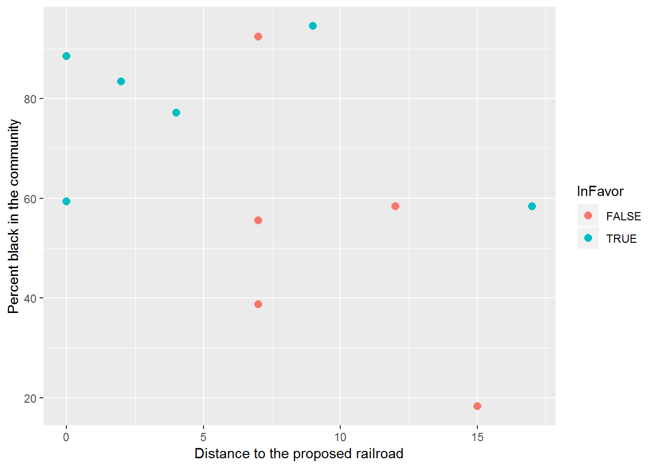
Figure 6.2: Scatterplot of distance from a proposed rail line and percent black in the community coded by whether the community was in favor of the referendum or not.

Recall that a model with two covariates has the form: \[\log(\textrm{odds}) = \log\left(\frac{p}{1-p}\right) = \beta_0+\beta_1X_1+\beta_2X_2.\] where \(p\) is the proportion of Yes votes in a community. In logistic regression, we expect the logits to be a linear function of \(X\), the predictors. To assess the linearity assumption, we construct empirical logit plots, where “empirical” means “based on sample data.” Empirical logits are computed for each community by taking \(\log\left(\frac{\textrm{number of successes}}{\textrm{number of failures}}\right)\). In Figure 6.3, we see that the plot of empirical logits versus distance produces a plot that looks linear, as needed for the logistic regression assumption. In contrast, the empirical logits by percent black reveal that Greensboro deviates quite a bit from the otherwise linear pattern; this suggests that Greensboro is an outlier and possibly an influential point. Greensboro has 99.2% voting yes with only 59.4% black.

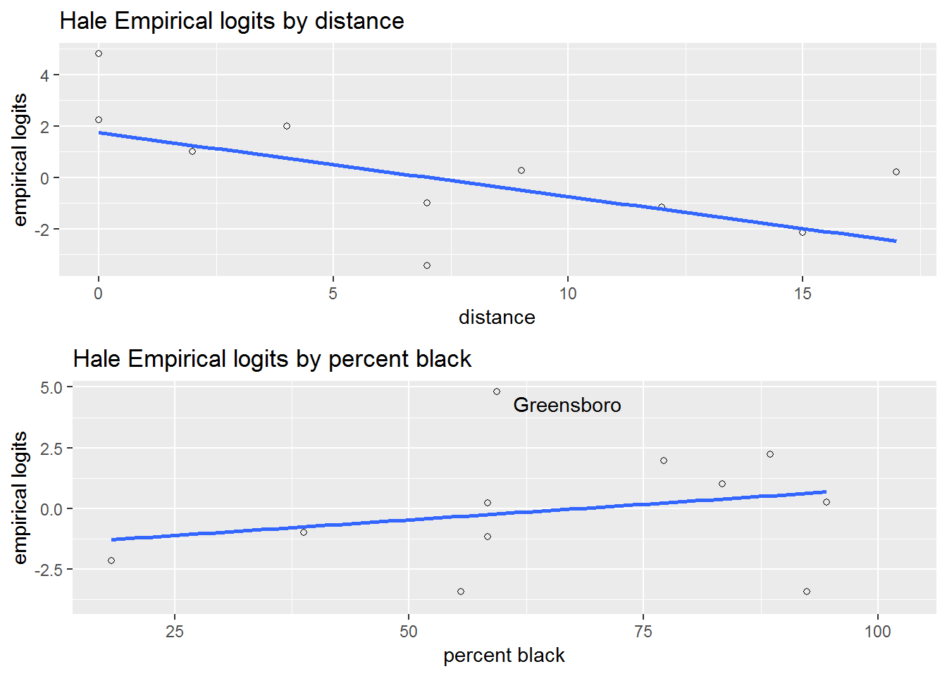
Figure 6.3: Empirical logit plots for the Railroad Referendum data.

In addition to examining how the response correlates with the predictors, it is a good idea to determine whether the predictors correlate with one another. Here the correlation between distance and percent black is negative and moderately strong with \(r = -0.49\). We’ll watch to see if the correlation affects the stability of our odds ratio estimates.

6.5.3 Initial Models

The first model includes only one covariate, distance.

glm(formula = cbind(YesVotes, NumVotes - YesVotes) ~ distance, 
    family = binomial, data = rrHale.df)

Coefficients:
            Estimate Std. Error z value Pr(>|z|)    
(Intercept)  3.30927    0.11313   29.25   <2e-16 ***
distance    -0.28758    0.01302  -22.09   <2e-16 ***
---
    Null deviance: 988.45  on 10  degrees of freedom
Residual deviance: 318.44  on  9  degrees of freedom
AIC: 360.73

Our estimated binomial regression model is: \[\log\left(\frac{\hat{p}_i}{1-\hat{p}_i}\right)=3.309-0.288 (\textrm{distance}_i)\] where \(\hat{p}_i\) is the estimated proportion of Yes votes in community \(i\). The estimated odds ratio for distance, that is the exponentiated coefficient for distance, in this model is \(e^{-0.288}=0.750\). It can be interpreted as follows: for each additional mile from the proposed railroad, the support (odds of a Yes vote) declines by 25.0%.

The covariate pctBlack is then added to the first model.

glm(formula = cbind(YesVotes, NumVotes - YesVotes) ~ distance + 
    pctBlack, family = binomial, data = rrHale.df)

Coefficients:
             Estimate Std. Error z value Pr(>|z|)    
(Intercept)  4.222021   0.296963  14.217  < 2e-16 ***
distance    -0.291735   0.013100 -22.270  < 2e-16 ***
pctBlack    -0.013227   0.003897  -3.394 0.000688 ***
---
    Null deviance: 988.45  on 10  degrees of freedom
Residual deviance: 307.22  on  8  degrees of freedom
AIC: 351.51

Despite the somewhat strong negative correlation between percent black and distance, the estimated odds ratio for distance remains approximately the same in this new model (OR \(= e^{-0.29} = 0.747\)); controlling for percent black does little to change our estimate of the effect of distance. For each additional mile from the proposed railroad, odds of a Yes vote declines by 25.3% after adjusting for the racial composition of a community. We also see that, for a fixed distance from the proposed railroad, the odds of a Yes vote declines by 1.3% (OR \(= e^{-.0132} = .987\)) for each additional percent black in the community.

6.5.4 Tests for significance of model coefficients

Do we have statistically significant evidence that support for the railroad referendum decreases with higher proportions of black residents in a community, after accounting for the distance a community is from the railroad line? As discussed in Section 4.4.3 with Poisson regression, there are two primary approaches to testing signficance of model coefficients: Drop-in-deviance test to compare models and Wald test for a single coefficient.

With our larger model given by \(\log\left(\frac{p_i}{1-p_i}\right) = \beta_0+\beta_1(\textrm{distance}_i)+\beta_2(\textrm{pctBlack}_i)\), the Wald test produces a highly significant p-value (\(Z=\frac{-0.0132}{0.0039}= -3.394\), \(p=.00069\)) indicating significant evidience that support for the railroad referendum decreases with higher proportions of black residents in a community, after adjusting for the distance a community is from the railroad line.

The drop in deviance test would compare the larger model above to the reduced model \(\log\left(\frac{p_i}{1-p_i}\right) = \beta_0+\beta_1(\textrm{distance}_i)\) by comparing residual deviances from the two models.

anova(model.HaleD, model.HaleBD, test = "Chisq")

Analysis of Deviance Table

Model 1: cbind(YesVotes, NumVotes - YesVotes) ~ distance
Model 2: cbind(YesVotes, NumVotes - YesVotes) ~ distance + pctBlack
  Resid. Df Resid. Dev Df Deviance  Pr(>Chi)    
1         9     318.44                          
2         8     307.22  1   11.222 0.0008083 ***
---
Signif. codes:  0 '***' 0.001 '**' 0.01 '*' 0.05 '.' 0.1 ' ' 1

The drop-in-deviance test statistic is \(318.44 - 307.22 = 11.22\) on \(9 - 8 = 1\) df, producing a p-value of .00081, in close agreement with the Wald test.

A third approach to determining significance of \(\beta_2\) would be to generate a 95% confidence interval and then checking if 0 falls within the interval or, equivalently, if 1 falls within a 95% confidence interval for \(e^{\beta_2}.\) The next section describes two approaches to producing a confidence interval for coefficients in logistic regression models.

6.5.5 Confidence intervals for model coefficients

Since the Wald statistic follows a normal distribution with \(n\) large, we could generate a Wald-type (normal-based) confidence interval for \(\beta_2\) using: \[\hat\beta_2 \pm 1.96\cdot\textrm{SE}(\hat\beta_2)\] and then exponentiating endpoints if we prefer a confidence interval for the odds ratio \(e^{\beta_2}\). In this case, \[\begin{eqnarray} 95\% \textrm{ CI for } &\beta_2 & = & \hat\beta_2 \pm 1.96 \cdot \textrm{SE}(\hat\beta_2) \\ & & = & -0.0132 \pm 1.96 \cdot 0.0039 \\ & & = & -0.0132 \pm 0.00764 \\ & & = & (-0.0208, -0.0056) \\ 95\% \textrm{ CI for } &e^{\beta_2} & = & (e^{-0.0208}, e^{-0.0056}) \\ & & = & (.979, .994) \\ 95\% \textrm{ CI for } &e^{10\beta_2} & = & (e^{-0.208}, e^{-0.056}) \\ & & = & (.812, .946) \end{eqnarray}\]

Thus, we can be 95% confident that a 10% increase in the proportion of black residents is associated with a 5.4% to 18.8% decrease in the odds of a Yes vote for the railroad referendum. This same relationship could be expressed as between a 0.6% and a 2.1% decrease in odds for each 1% increase in the black population, or between a 5.7% (\(1/e^{-.056}\)) and a 23.1% (\(1/e^{-.208}\)) increase in odds for each 10% decrease in the black population, after adjusting for distance. Of course, with \(n=11\), we should be cautious about relying on a Wald-type interval in this example.

Another approach available in R is the profile likelihood method, similar to Chapter 4.

exp(confint(model.HaleBD))

                 2.5 %      97.5 %
(Intercept) 38.2284603 122.6115988
distance     0.7276167   0.7659900
pctBlack     0.9793819   0.9944779

In the model with distance and pctBlack, the profile likelihood 95% confidence interval for \(e^{\beta_2}\) is (.979, .994), which is approximately equal to the Wald-based interval despite the small sample size. We can also confirm the statistically significant association between percent black and odds of voting Yes (after controlling for distance), because 1 is not a plausible value of \(e^{\beta_2}\) (where an odds ratio of 1 would imply that the odds of voting Yes do not change with percent black).

6.5.6 Testing for goodness of fit

As in Section 4.4.9, we can evaluate the goodness of fit for our model by comparing the residual deviance (307.22) to a \(\chi^2\) distribution with \(n-p\) (8) degrees of freedom.

1-pchisq(307.2173, 8)

[1] 0

The model with pctBlack and distance has statistically significant evidence of lack of fit (\(p<.001\)).

Similar to the Poisson regression models, this lack of fit could result from (a) missing covariates, (b) outliers, or (c) overdispersion. We will first attempt to address (a) by fitting a model with an interaction between distance and percent black, to determine whether the effect of racial composition differs based on how far a community is from the proposed railroad.

glm(formula = cbind(YesVotes, NumVotes - YesVotes) ~ distance + 
    pctBlack + distance:pctBlack, family = binomial, data = rrHale.df)

Coefficients:
                    Estimate Std. Error z value Pr(>|z|)    
(Intercept)        7.5509017  0.6383697  11.828  < 2e-16 ***
distance          -0.6140052  0.0573808 -10.701  < 2e-16 ***
pctBlack          -0.0647308  0.0091723  -7.057 1.70e-12 ***
distance:pctBlack  0.0053665  0.0008984   5.974 2.32e-09 ***
---
    Null deviance: 988.45  on 10  degrees of freedom
Residual deviance: 274.23  on  7  degrees of freedom
AIC: 320.53

Analysis of Deviance Table

Model 1: cbind(YesVotes, NumVotes - YesVotes) ~ distance + pctBlack
Model 2: cbind(YesVotes, NumVotes - YesVotes) ~ distance + pctBlack + 
    distance:pctBlack
  Resid. Df Resid. Dev Df Deviance  Pr(>Chi)    
1         8     307.22                          
2         7     274.23  1   32.984 9.294e-09 ***
---
Signif. codes:  0 '***' 0.001 '**' 0.01 '*' 0.05 '.' 0.1 ' ' 1

We have statistically significant evidence (Wald test: \(Z = 5.974, p<.001\); Drop in deviance test: \(\chi^2=32.984, p<.001\)) that the effect of the proportion of the community that is black on the odds of voting Yes depends on the distance of the community from the proposed railroad.

To interpret the interaction coefficient in context, we will compare two cases: one where a community is right on the proposed railroad (distance = 0), and the other where the community is 15 miles away (distance = 15). The significant interaction implies that the effect of pctBlack should differ in these two cases. In the first case, the coefficient for pctBlack is -0.0647, while in the second case, the relevant coefficient is \(-0.0647+15(.00537) = 0.0158\). Thus, for a community right on the proposed railroad, a 1% increase in percent black is associated with a 6.3% (\(e^{-.0647}=.937\)) decrease in the odds of voting Yes, while for a community 15 miles away, a 1% increase in percent black is associated with a (\(e^{.0158}=1.016\)) 1.6% increase in the odds of voting Yes. A significant interaction term doesn’t always imply a change in the direction of the association, but it does here.

Because our interaction model still exhibits lack of fit (residual deviance of 274.23 on just 7 df), and because we have used the covariates at our disposal, we will assess this model for potential outliers and overdispersion by examining the model’s residuals.

6.5.7 Residuals for Binomial Regression

With OLS, residuals were used to assess model assumptions and identify outliers. For binomial regression, two different types of residuals are typically used. One residual, the Pearson residual, has a form similar to that used with OLS. Specifically, the Pearson residual is calculated using: \[\begin{equation} \textrm{Pearson residual}_i = \frac{\textrm{actual count}-\textrm{predicted count}}{\textrm{SD of count}} = \frac{Y_i-m_i\hat{p_i}}{\sqrt{m_i\hat{p_i}(1-\hat{p_i})}} \tag{6.11} \end{equation}\]

where \(m_i\) is the number of trials for the \(i^{th}\) observation and \(\hat{p}_i\) is the estimated probability of success for that same observation.

A deviance residual is an alternative residual for binomial regression based on the discrepancy between the observed values and those estimated using the likelihood. A deviance residual can be calculated for each observation using: \[\begin{equation} \textrm{d}_i = \textrm{sign}(Y_i-m_i\hat{p_i})\sqrt{2[Y_i \log\left(\frac{Y_i}{m_i \hat{p_i}}\right)+ (m_i - Y_i) \log\left(\frac{m_i - Y_i}{m_i - m_i \hat{p_i}}\right)]} \tag{6.12} \end{equation}\]

Where \(\textrm{sign}(x)\) is defined such that: \[ \textrm{sign}(x) = \begin{cases} 1 & \textrm{if }\ x > 0 \\ -1 & \textrm{if }\ x < 0 \\ 0 & \textrm{if }\ x = 0\end{cases}\]

When the number of trials is large for all of the observations and the models are appropriate, both sets of residuals should follow a standard normal distribution.

The sum of the individual deviance residuals is referred to as the deviance or residual deviance. The deviance is used to assess the model. As the name suggests, a model with a small deviance is preferred. In the case of binomial regression, when the denominators, \(m_i\), are large and a model fits, the residual deviance follows a \(\chi^2\) distribution with \(n-p\) degrees of freedom (the residual degrees of freedom). Thus for a good fitting model the residual deviance should be approximately equal to its corresponding degrees of freedom. When binomial data meets these conditions, the deviance can be used for a goodness-of-fit test. The p-value for lack-of-fit is the proportion of values from a \(\chi_{n-p}^2\) that are greater than the observed residual deviance.

We begin a residual analysis of our interaction model by plotting the residuals against the fitted values in Figure 6.4. This kind of plot for binomial regression would produce two linear trends with similar negative slopes if there were equal sample sizes \(m_i\) for each observation.

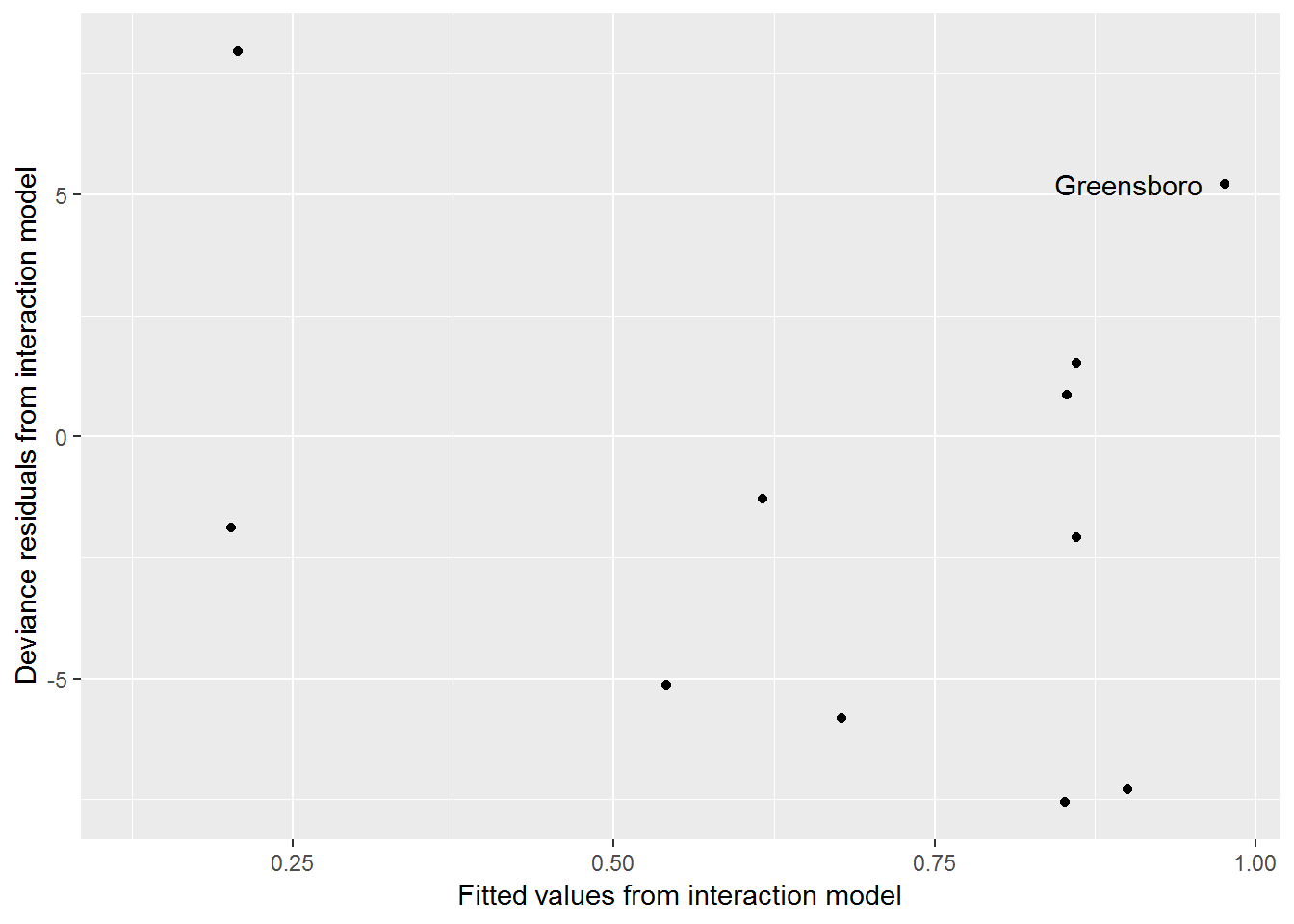
Figure 6.4: Fitted values by residuals for the interaction model for the Railroad Referendum data.

From this residual plot, Greensboro does not stand out as an outlier. If it did, we could remove Greensboro and refit our interaction model, checking to see if model coefficients changed in a noticeable way. Instead, we will continue to include Greensboro in our modeling efforts. Because the large residual deviance cannot be explained by outliers, and given we have included all of the covariates at hand as well as an interaction term, the observed binomial counts are likely overdispersed. This means that they exhibit more variation than the model would suggest, and we must consider ways to handle this overdispersion.

6.5.8 Overdispersion

Similarly to Poisson regression we can adjust for overdispersion in binomial regression. With overdispersion there is extra-binomial variation, so the actual variance will be greater than the variance of a binomial variable, \(np(1-p)\). One way to adjust for overdispersion is to estimate a multiplier (dispersion parameter), \(\hat{\phi}\), for the variance that will inflate it and reflect the reduction in the amount of information we would otherwise have with independent observations. We used a similar approach to adjust for overdispersion in a Poisson regression model in Section 4.9, and we will use the same estimate here: \(\hat\phi=\frac{\sum(\textrm{Pearson residuals})^2}{n-p}\).

When overdispersion is adjusted for in this way, we can no longer use maximum likelihood to fit our regression model; instead we use a quasi-likelihood approach. Quasi-likelihood is similar to likelihood-based inference, but because the model uses the dispersion parameter, it is not a binomial model with a true likelihood. R offers quasi-likelihood as an option when model fitting. The quasi-likelihood approach will yield the same coefficient point estimates as maximum likelihood; however, the variances will be larger in the presence of overdispersion (assuming \(\phi>1\)). We will see other ways in which to deal with overdispersion and clusters in the remaining chapters in the book, but the following describes how overdispersion is accounted for using \(\hat{\phi}\):

Summary: Accounting for Overdispersion

• Use the dispersion parameter \(\hat\phi=\frac{\sum(\textrm{Pearson residuals})^2}{n-p}\) to inflate standard errors of model coefficients
• Wald test statistics: multiply the standard errors by \(\sqrt{\hat{\phi}}\) so that \(\textrm{SE}_\textrm{Q}(\hat\beta)=\sqrt{\hat\phi}\cdot\textrm{SE}(\hat\beta)\) and conduct tests using the \(t\)-distribution
• CIs use the adjusted standard errors and multiplier based on \(t\), so they are thereby wider: \(\hat\beta \pm t_{n-p} \cdot \textrm{SE}_\textrm{Q}(\hat\beta)\)
• Drop-in-deviance test statistic comparing Model 1 (larger model with \(p\) parameters) to Model 2 (smaller model with \(q<p\) parameters) = \[\begin{equation} F = \frac{1}{\hat\phi} \cdot \frac{D_2 - D_1}{p-q} \tag{6.13} \end{equation}\] where \(D_1\) and \(D_2\) are the residual deviances for models 1 and 2 respectively and \(p-q\) is the difference in the number of parameters for the two models. Note that both \(D_2-D_1\) and \(p-q\) are positive. This test statistic is compared to an F-distribution with \(p-q\) and \(n-p\) degrees of freedom.

Output for a model which adjusts our interaction model for overdispersion appears below, where \(\hat{\phi}=51.6\) is used to adjust the standard errors for the coefficients and the drop-in-deviance tests during model building. Standard errors will be inflated by a factor of \(\sqrt{51.6}=7.2\). As a results, there are no significant terms in the adjusted interaction model below.

glm(formula = cbind(YesVotes, NumVotes - YesVotes) ~ distance + 
    pctBlack + distance:pctBlack, family = quasibinomial, data = rrHale.df)

Coefficients:
                   Estimate Std. Error t value Pr(>|t|)
(Intercept)        7.550902   4.585464   1.647    0.144
distance          -0.614005   0.412171  -1.490    0.180
pctBlack          -0.064731   0.065885  -0.982    0.359
distance:pctBlack  0.005367   0.006453   0.832    0.433

(Dispersion parameter for quasibinomial family taken to be 51.5967)

    Null deviance: 988.45  on 10  degrees of freedom
Residual deviance: 274.23  on  7  degrees of freedom

We therefore remove the interaction term and refit the model, adjusting for the extra-binomial variation that still exists.

glm(formula = cbind(YesVotes, NumVotes - YesVotes) ~ distance + 
    pctBlack, family = quasibinomial, data = rrHale.df)

Coefficients:
            Estimate Std. Error t value Pr(>|t|)  
(Intercept)  4.22202    1.99031   2.121   0.0667 .
distance    -0.29173    0.08780  -3.323   0.0105 *
pctBlack    -0.01323    0.02612  -0.506   0.6262  
---
(Dispersion parameter for quasibinomial family taken to be 44.9194)

    Null deviance: 988.45  on 10  degrees of freedom
Residual deviance: 307.22  on  8  degrees of freedom

By removing the interaction term and using the overdispersion parameter, we see that distance is significantly associated with support, but percent black is no longer significant after adjusting for distance.

Because quasi-likelihood methods do not change estimated coefficients, we still estimate a 25% decline \((1-e^{-0.292})\) in support for each additional mile from the proposed railroad (odds ratio of .75).

exp(confint(model.HaleBDq))

                2.5 %       97.5 %
(Intercept) 1.3608623 5006.7224182
distance    0.6091007    0.8710322
pctBlack    0.9365625    1.0437861

While we previously found a 95% confidence interval for the odds ratio of (.728, .766), our confidence interval is now much wider: (.609, .871). Appropriately accounting for overdispersion has changed both the significance of certain terms and the precision of our coefficient estimates.

6.5.9 Summary

We began by fitting a logistic regression model with distance alone. Then we added covariate pctBlack, and the Wald-type test and the drop-in-deviance provided strong support for the addition of pctBlack to the model. The model with distance and pctBlack had a large residual deviance suggesting an ill-fitted model. When we looked at the residuals, we saw that Greensboro is an extreme observation. Models without Greensboro were fitted and compared to our initial models. Seeing no appreciable improvement or differences with Greensboro removed, we left it in the model. There remained a large residual deviance so we attempted to account for it by using an estimated dispersion parameter similar to Section 4.9 with Poisson regression. The final model included distance and percent black, although percent black was no longer significant after adjusting for overdispersion.

6.6 Least Squares Regression vs. Logistic Regression

\[ \underline{\textrm{Response}} \\ \mathbf{OLS:}\textrm{ normal} \\ \mathbf{Binomial\ Regression:}\textrm{ number of successes in n trials} \\ \textrm{ } \\ \underline{\textrm{Variance}} \\ \mathbf{OLS:}\textrm{ Equal for each level of}\ X \\ \mathbf{Binomial\ Regression:}\ np(1-p)\textrm{ for each level of}\ X \\ \textrm{ } \\ \underline{\textrm{Model Fitting}} \\ \mathbf{OLS:}\ \mu=\beta_0+\beta_1x \textrm{ using Least Squares}\\ \mathbf{Binomial\ Regression:}\ \log\left(\frac{p}{1-p}\right)=\beta_0+\beta_1x \textrm{ using Maximum Likelihood}\\ \textrm{ } \\ \underline{\textrm{EDA}} \\ \mathbf{OLS:}\textrm{ plot $X$ vs. $Y$; add line} \\ \mathbf{Binomial\ Regression:}\textrm{ find $\log(\textrm{odds})$ for several subgroups; plot vs. $X$} \\ \textrm{ } \\ \underline{\textrm{Comparing Models}} \\ \mathbf{OLS:}\textrm{ extra sum of squares F-tests; AIC/BIC} \\ \mathbf{Binomial\ Regression:}\textrm{ Drop in Deviance tests; AIC/BIC} \\ \textrm{ } \\ \underline{\textrm{Interpreting Coefficients}} \\ \mathbf{OLS:}\ \beta_1=\textrm{ change in }\mu_y\textrm{ for unit change in $X$} \\ \mathbf{Binomial\ Regression:}\ e^{\beta_1}=\textrm{ percent change in odds for unit change in $X$} \]

6.7 Case Study: Trying to Lose Weight

The final case study uses individual-specific information so that our response, rather than the number of successes out of some number of trials, is simply a binary variable taking on values of 0 or 1 (for failure/success, no/yes, etc.). This type of problem—binary logistic regression—is exceedingly common in practice. Here we examine characteristics of young people who are trying to lose weight. The prevalence of obesity among US youth suggests that wanting to lose weight is sensible and desirable for some young people such as those with a high body mass index (BMI). On the flip side, there are young people who do not need to lose weight but make ill-advised attempts to do so nonetheless. A multitude of studies on weight loss focus specifically on youth and propose a variety of motivations for the young wanting to lose weight; athletics and the media are two commonly cited sources of motivation for losing weight for young people.

Sports have been implicated as a reason for young people wanting to shed pounds, but not all studies are consistent with this idea. For example, a study by Martinsen et al. (2009) reported that, despite preconceptions to the contrary, there was a higher rate of self-reported eating disorders among controls (non-elite athletes) as opposed to elite athletes. Interestingly, the kind of sport was not found to be a factor, as participants in leanness sports (for example, distance running, swimming, gymnastics, dance, and diving) did not differ in the proportion with eating disorders when compared to those in non-leanness sports. So, in our analysis, we will not make a distinction between different sports.

Other studies suggest that mass media is the culprit. They argue that students’ exposure to unrealistically thin celebrities may provide unhealthy motivation for some, particularly young women, to try to slim down. An examination and analysis of a large number of related studies (referred to as a meta-analysis) (Grabe, Hyde, and Ward 2008) found a strong relationship between exposure to mass media and the amount of time that adolescents spend talking about what they see in the media, deciphering what it means, and figuring out how they can be more like the celebrities.

We are interested in the following questions: Are the odds that young females report trying to lose weight greater that the odds that males do? Is increasing BMI is associated with an interest in losing weight, regardless of sex? Does sports participation increase the desire to lose weight? Is media exposure is associated with more interest in losing weight?

We have sample of 500 teens from data collected in 2009 through the U.S. Youth Risk Behavior Surveillance System (YRBSS) (Centers for Disease Control and Prevention 2009). The YRBSS is an annual national school-based survey conducted by the Centers for Disease Control and Prevention (CDC) and state, territorial, and local education and health agencies and tribal governments. More information on this survey can be found here.

6.7.1 Data Organization

Here are the three questions from the YRBSS we use for our investigation:

Q66. Which of the following are you trying to do about your weight?

• A. Lose weight
• B. Gain weight
• C. Stay the same weight
• D. I am not trying to do anything about my weight

Q81. On an average school day, how many hours do you watch TV?

• A. I do not watch TV on an average school day
• B. Less than 1 hour per day
• C. 1 hour per day
• D. 2 hours per day
• E. 3 hours per day
• F. 4 hours per day
• G. 5 or more hours per day

Q84. During the past 12 months, on how many sports teams did you play? (Include any teams run by your school or community groups.)

• A. 0 teams
• B. 1 team
• C. 2 teams
• D. 3 or more teams

Answers to Q66 are used to define our response variable: Y = 1 corresponds to “(A) trying to lose weight”, while Y = 0 corresponds to the other non-missing values. Q84 provides information on students’ sports participation and is treated as numerical, 0 through 3, with 3 representing 3 or more. As a proxy for media exposure we use answers to Q81 as numerical values 0, 0.5, 1, 2, 3, 4, and 5, with 5 representing 5 or more. Media exposure and sports participation are also considered as categorical factors, that is, as variables with distinct levels which can be denoted by indicator variables as opposed to their numerical values.

BMI is included in this study as the percentile for a given BMI for members of the same sex. This facilitates comparisons when modeling with males and females. We will use the terms BMI and BMI percentile interchangeably with the understanding that we are always referring to the percentile.

With our sample, we use only the cases that include all of the data for these four questions. This is referred to as a complete case analysis. That brings our sample of 500 to 426. There are limitations of complete case analyses that we address in the Discussion.

6.7.2 Exploratory Data Analysis

Nearly half (44.5%) of our sample of 426 youth report that they are trying to lose weight, 49.9% percent of the sample are females, and 56.6% play on one or more sports teams. 9.3 percent report that they do not watch any TV on school days, whereas another 9.3% watched 5 or more hours each day. Interestingly, the median BMI percentile for our 426 youth is 70. The most dramatic difference in the proportions of those who are trying to lose weight is by sex; 58% of the females want to lose weight in contrast to only 31% of the males (see Figure 6.5). This provides strong support for the inclusion of a sex term in every model considered.

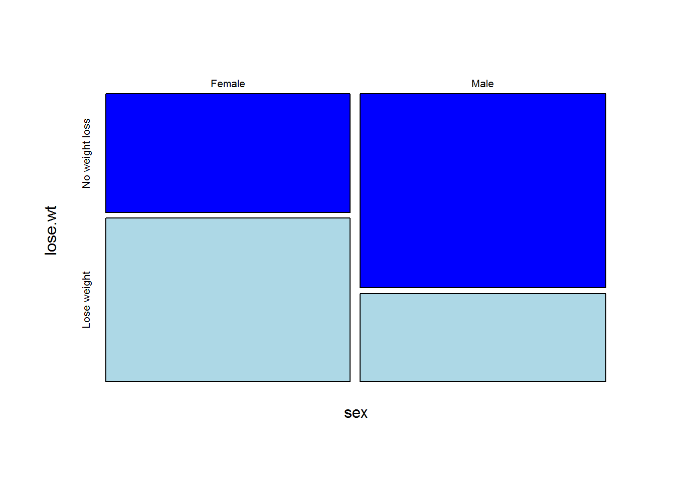
Figure 6.5: Weight loss plans vs. Sex

Table 6.3: Mean BMI percentile by sex and desire to lose weight.

Sex	Weight loss status	mean BMI percentile	SD	n
Female	No weight loss	48.2	26.2	90
	Lose weight	76.3	19.5	124
Male	No weight loss	54.9	28.6	148
	Lose weight	84.4	17.7	67

Table 6.3 displays the mean BMI of those wanting and not wanting to lose weight for males and females. The mean BMI is greater for those trying to lose weight compared to those not trying to lose weight, regardless of sex. The size of the difference is remarkably similar for the two sexes.

If we consider including a BMI term in our model(s), the logit should be linearly related to BMI. We can investigate this assumption by constructing an empirical logit plot. In order to calculate empirical logits, we first divide our data by sex. Within each sex, we generate 10 groups of equal sizes, the first holding the bottom 10% in BMI percentile for that sex, the second holding the next lowest 10%, etc.. Within each group, we calculate the proporton, \(\hat{p}\) that reported wanting to lose weight, and then the empirical log odds, \(log(\frac{\hat{p}}{1-\hat{p}})\), that a young person in that group wants to lose weight.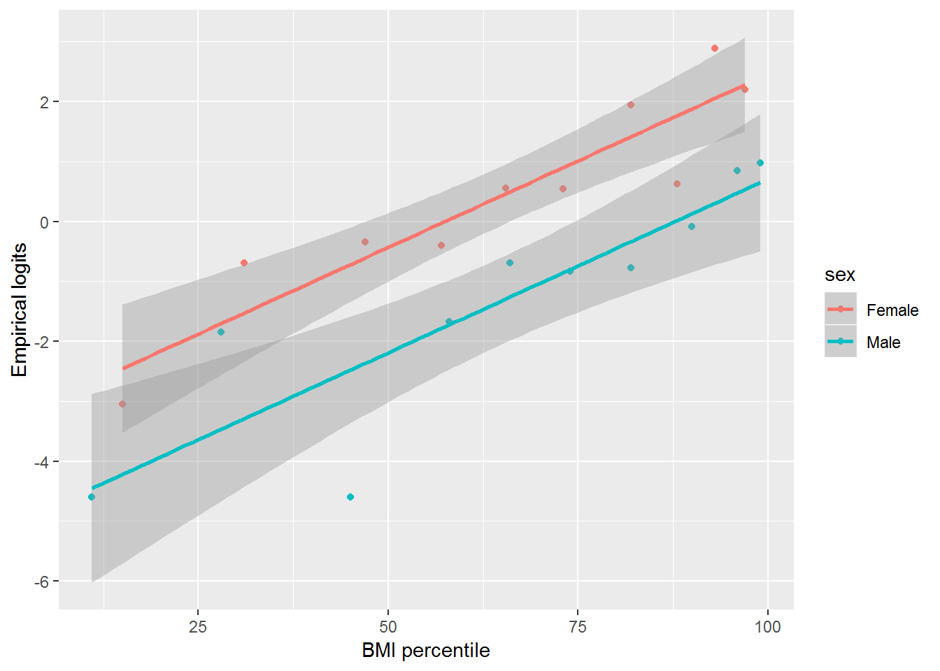

Figure 6.6: Empirical logits of trying to lose weight by BMI and Sex.

Figure 6.6 presents the empirical logits for the BMI intervals by sex. Both males and females exhibit an increasing linear trend on the logit scale indicating that increasing BMI is associated a greater desire to lose weight and that modeling log odds as a linear function of BMI is reasonable. The slope for the females appears to be similar to the slope for males, so we do not need to consider an interaction term between BMI and sex in the model.

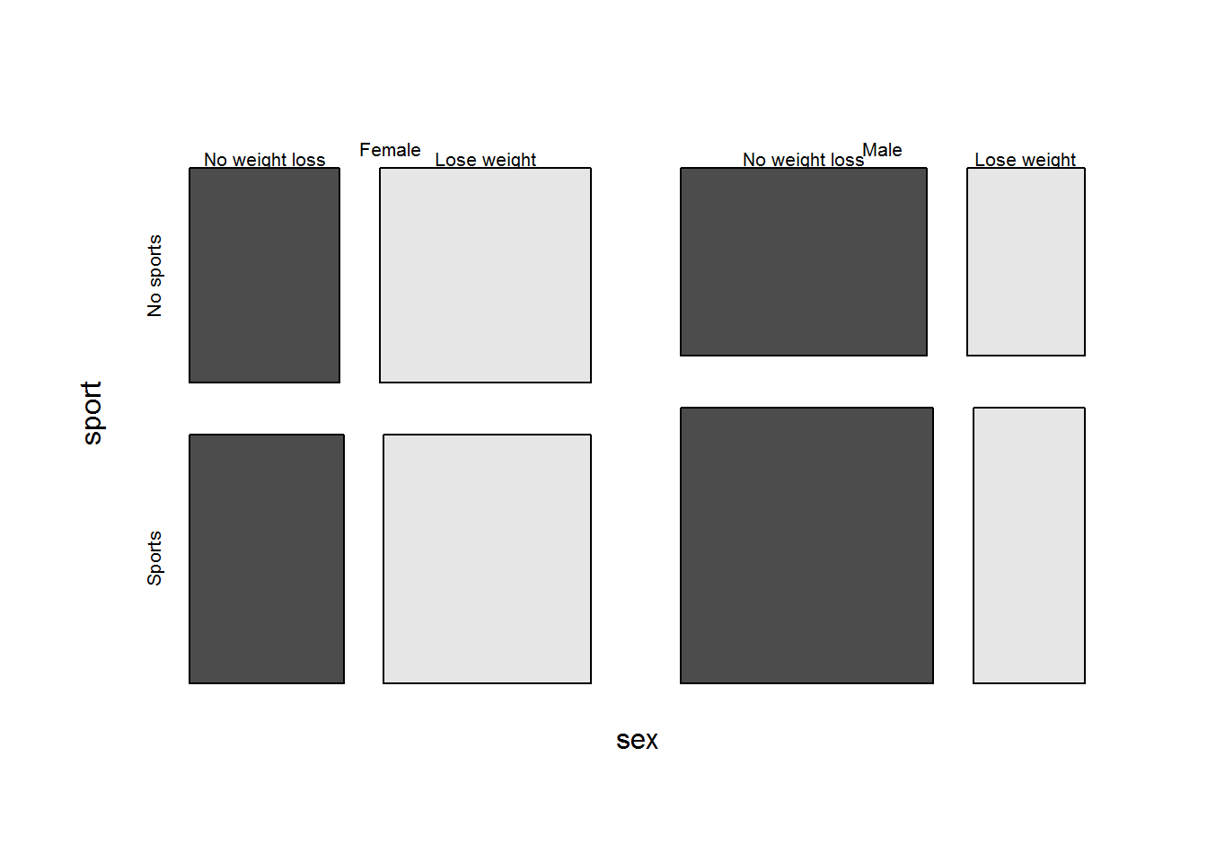
Figure 6.7: Weight loss plans vs. sex and sports participation

Out of those who play sports, 43% want to lose weight whereas 46% want to lose weight among those who do not play sports. Figure 6.7 compares the proportion of respondents who want to lose weight by their sex and sport participation. The data suggest that sports participation is associated with the same or even a slightly lower desire to lose weight, contrary to what had originally been hypothesized. While the overall levels of those wanting to lose weight differ considerably between the sexes, the differences between those in and out of sports within sex appear to be very small. A term for sports participation or number of teams will be considered, but there is not compelling evidence that an interaction term will be needed.

It was posited that increased exposure to media, here measured as hours of TV daily, is associated with increased desire to lose weight, particularly for females. Overall, the percentage who want to lose weight ranges from 35% of those watching 5 hours of TV per day to 52% among those watching 3 hours daily. There is minimal variation in the proportion wanting to lose weight with both sexes combined. However, we are more interested in differences between the sexes (see Figure 6.8). We create empirical logits using the proportion of students trying to lose weight for each level of hours spent watching daily and look at the trends in the logits separately for males and females. From Figure 6.9, there does not appear to be a linear relationship for males or females.

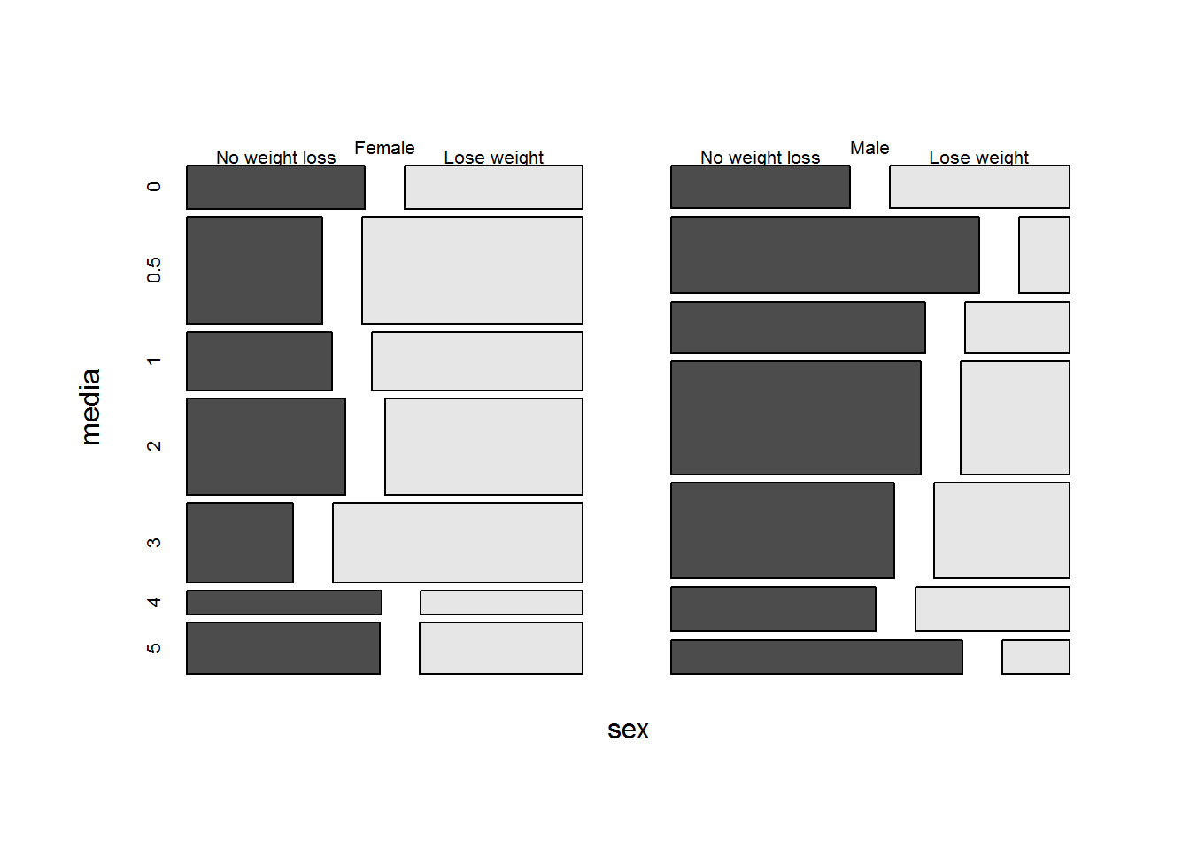
Figure 6.8: Weight loss plans vs. daily hours of TV and sex.

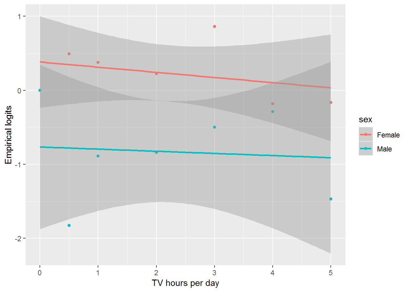
Figure 6.9: Empirical logits for the odds of trying to lose weight by TV watching and sex.

6.7.3 Initial Models

Our strategy for modeling is to use our questions of interest and what we have learned in the exploratory data analysis. For each model we interpret the coefficient of interest, look at the corresponding Wald test and, as a final step, compare the deviances for the different models we considered.

We first use a model where sex is our only predictor.

glm(formula = lose.wt.01 ~ female, family = binomial, data = risk2009)

Coefficients:
            Estimate Std. Error z value Pr(>|z|)    
(Intercept)  -0.7925     0.1472  -5.382 7.36e-08 ***
female        1.1130     0.2021   5.506 3.67e-08 ***
---
    Null deviance: 589.56  on 428  degrees of freedom
Residual deviance: 558.01  on 427  degrees of freedom
AIC: 562.01

Our estimated binomial regression model is: \[\log\left(\frac{{p}}{1-{p}}\right)=-0.79+1.11 (\textrm{female})\] where \({p}\) is the estimated proportion of youth wanting to lose weight. We can interpret the coefficient on female by exponentiating \(e^{1.1130} = 3.04\) (95% CI = \((2.05, 4.54)\)) indicating that the odds of a female trying to lose weight is over three times the odds of a male trying to lose weight (\(Z=5.506\), \(p=3.67e-08\)). We retain sex in the model and consider adding the BMI percentile:

glm(formula = lose.wt.01 ~ female + bmipct, family = binomial, 
    data = risk2009)

Coefficients:
             Estimate Std. Error z value Pr(>|z|)    
(Intercept) -4.458822   0.471411  -9.458  < 2e-16 ***
female       1.544968   0.249009   6.204 5.49e-10 ***
bmipct       0.050915   0.005615   9.067  < 2e-16 ***
---
    Null deviance: 589.56  on 428  degrees of freedom
Residual deviance: 434.88  on 426  degrees of freedom
AIC: 440.88

We see that there is statistically significant evidence (\(Z=9.067, p<.001\)) that BMI is positively associated with the odds of trying to lose weight, after controlling for sex. Clearly BMI percentile belongs in the model with sex.

Our estimated binomial regression model is: \[\log\left(\frac{{p}}{1-{p}}\right)= -4.46+1.54\textrm{female}+0.051\textrm{bmipct}\]

To interpret the coefficient on bmipct, we will consider a 10 unit increase in bmipct. Because \(e^{10*0.0509}=1.664\), then there is an estimated 66.4% increase in the odds of wanting to lose weight for each additional 10 percentile points of BMI for members of the same sex. Just as we had done in other multiple regression models we need to interpret our coefficient given that the other variables remain constant. An interaction term for BMI by sex was tested (not shown) and it was not significant (\(Z=-0.405\), \(p=0.6856\)), so the effect of BMI does not differ by sex.

We next add sport to our model. Sports participation was considered for inclusion in the model in three ways: an indicator of sports participation (0 = no teams, 1 = one or more teams), treating the number of teams (0, 1, 2, or 3) as numeric, and treating the number of teams as a factor. The models below treat sports participation using an indicator variable, but all three models produced similar results.

glm(formula = lose.wt.01 ~ female + bmipct + sport, family = binomial, 
    data = risk2009)

Coefficients:
             Estimate Std. Error z value Pr(>|z|)    
(Intercept) -4.401651   0.495445  -8.884  < 2e-16 ***
female       1.540816   0.249349   6.179 6.44e-10 ***
bmipct       0.050852   0.005609   9.066  < 2e-16 ***
sportSports -0.086068   0.238976  -0.360    0.719    

    Null deviance: 589.56  on 428  degrees of freedom
Residual deviance: 434.75  on 425  degrees of freedom

glm(formula = lose.wt.01 ~ female + bmipct + sport + female:sport + 
    bmipct:sport, family = binomial, data = risk2009)

Coefficients:
                    Estimate Std. Error z value Pr(>|z|)    
(Intercept)        -4.703220   0.737180  -6.380 1.77e-10 ***
female              1.715041   0.409666   4.186 2.83e-05 ***
bmipct              0.053789   0.008353   6.439 1.20e-10 ***
sportSports         0.430530   0.966620   0.445    0.656    
female:sportSports -0.280653   0.516786  -0.543    0.587    
bmipct:sportSports -0.005232   0.011372  -0.460    0.645    

    Null deviance: 589.56  on 428  degrees of freedom
Residual deviance: 434.37  on 423  degrees of freedom

Sports teams were not significant in any of these models, nor were interaction terms (sex by sports) and (bmipct by sports). As a result, sports participation was no longer considered for inclusion in the model.

We last look at adding media to our model.

glm(formula = lose.wt.01 ~ bmipct + female + media, family = binomial, 
    data = risk2009)

Coefficients:
             Estimate Std. Error z value Pr(>|z|)    
(Intercept) -4.355420   0.489782  -8.893  < 2e-16 ***
bmipct       0.051153   0.005642   9.066  < 2e-16 ***
female       1.538602   0.249167   6.175 6.62e-10 ***
media       -0.058406   0.078421  -0.745    0.456    
---
    Null deviance: 589.56  on 428  degrees of freedom
Residual deviance: 434.33  on 425  degrees of freedom
AIC: 442.33

Media is not a statistically significant term (\(p=0.456\), \(Z=-0.745\)). However, because our interest centers on how media may affect attempts to lose weight and how its effect might be different for females and males, we fit a model with a media term and a sex by media interaction term (not shown). Neither term was statistically significant, so we have no support in our data that media exposure as measured by hours spent watching TV is associated with the odds a teen is trying to lose weight after accounting for sex and BMI.

6.7.4 Drop-in-deviance Tests

Analysis of Deviance Table

Model 1: lose.wt.01 ~ female
Model 2: lose.wt.01 ~ female + bmipct
Model 3: lose.wt.01 ~ female + bmipct + sport
Model 4: lose.wt.01 ~ bmipct + female + media
  Resid. Df Resid. Dev Df Deviance Pr(>Chi)    
1       427     558.01                         
2       426     434.88  1  123.129   <2e-16 ***
3       425     434.75  1    0.130   0.7188    
4       425     434.33  0    0.426             
---
Signif. codes:  0 '***' 0.001 '**' 0.01 '*' 0.05 '.' 0.1 ' ' 1

       df      AIC
model1  2 562.0129
model2  3 440.8838
model3  4 442.7541
model4  4 442.3281

Comparing models using differences in deviances requires that the models be nested, meaning each smaller model is a simplified version of the larger model. In our case, Models 1, 2, and 4 are nested, as are Models 1, 2, and 3, but Models 3 and 4 cannot be compared using a drop-in-deviance test.

There is a large drop-in-deviance adding BMI to the model with sex (Model 1 to Model 2, 123.13), which is clearly statistically significant when compared to a \(\chi^2\) distribution with 1 df. The drop-in-deviance for adding an indicator variable for sports to the model with sex and BMI is only 434.88 - 434.75 = 0.13. There is a difference of a single parameter, so the drop-in-deviance would be compared to a \(\chi^2\) distribution with 1 df. The resulting \(p\)-value is very large (.7188) suggesting that adding an indicator for sports is not helpful once we’ve already accounted for BMI and sex. For comparing Models 3 and 4, one approach is to look at the AIC. In this case, the AIC is (barely) smaller for the model with media, providing evidence that the latter model is slightly preferable.

6.7.5 Model Discussion and Summary

We found that the odds of wanting to lose weight are considerably greater for females compared to males. In addition, respondents with greater BMI percentiles express a greater desire to lose weight for members of the same sex. Regardless of sex or BMI percentile, sports participation and TV watching are not associated with different odds for wanting to lose weight.

A limitation of this analysis is that we used complete cases in place of a method of imputing responses or modeling missingness. This reduced our sample from 500 to 429, and it may have introduced bias. For example, if respondents who watch a lot of TV were unwilling to reveal as much, and if they differed with respect to their desire to lose weight from those respondents who reported watching little TV, our inferences regarding the relationship between lots of TV and desire to lose weight may be biased.

Other limitations may result from definitions. Trying to lose weight is self-reported and may not correlate with any action undertaken to do so. The number of sports teams may not accurately reflect sports related pressures to lose weight. For example, elite athletes may focus on a single sport and be subject to greater pressures whereas athletes who casually participate in three sports may not feel any pressure to lose weight. Hours spent watching TV is not likely to encompass the totality of media exposure, particularly because exposure to celebrities occurs often online. Furthermore, this analysis does not explore in any detail maladaptions—inappropriate motivations for wanting to lose weight. For example, we did not focus our study on subsets of respondents with low BMI who are attempting to lose weight.

It would be instructive to use data science methodologies to explore the entire data set of 16,000 instead of sampling 500. However, the types of exploration and models used here could translate to the larger sample size.

Finally a limitation may be introduced as a result of the acknowledged variation in the administration of the YRBSS. States and local authorities are allowed to administer the survey as they see fit, which at times results in significant variation in sample selection and response.

6.8 Exercises

6.8.1 Conceptual Excersises:

1. List the explanatory and response variable(s) for each research question.

1. Are students with poor grades more likely to binge drink?
2. What is the chance you are accepted into medical school given your GPA and MCAT scores?
3. Does a single mom have a better chance of marrying the baby’s father if she has a boy?
4. Are students participating in sports in college more or less likely to graduate?
5. Is exposure to a particular chemical associated with a cancer diagnosis?

2. Interpret the odds ratios in the following abstract.

Day Care Centers and Respiratory Health (Nafstad et al. 1999)

Objective. To estimate the effects of the type of day care on respiratory health in preschool children.

Methods. A population-based cross-sectional study of Oslo children born in 1992 was conducted at the end of 1996. A self-administered questionnaire inquired about day care arrangements, environmental conditions, and family characteristics (n = 3853; response rate, 79%).

Results. In a logistic regression controlling for confounding, children in day care centers had more often nightly cough (adjusted odds ratio, 1.89; 95% confidence interval 1.34-2.67), and blocked or runny nose without common cold (1.55; 1.07-1.61) during the past 12 months compared with children in home care…

3. Construct a table and calculate the corresponding odds and odds ratios. Comment on the reported and calculated results in this New York Times article from Kolata (2009).

In November, the Centers for Disease Control and Prevention published a paper reporting that babies conceived with IVF, or with a technique in which sperm are injected directly into eggs, have a slightly increased risk of several birth defects, including a hole between the two chambers of the heart, a cleft lip or palate, an improperly developed esophagus and a malformed rectum. The study involved 9,584 babies with birth defects and 4,792 babies without. Among the mothers of babies without birth defects, 1.1 percent had used IVF or related methods, compared with 2.4 percent of mothers of babies with birth defects.

The findings are considered preliminary, and researchers say they believe IVF does not carry excessive risks. There is a 3 percent chance that any given baby will have a birth defect.

6.8.2 Guided Exercises

1. Soccer goals on target. Data comes from an article in Psychological Science (Roskes et al. 2011). The authors report on the success rate of penalty kicks that were on-target, so that either the keeper saved the shot or the shot scored, for FIFA World Cup shootouts between 1982 and 2010. They found that 18 out of 20 shots were scored when the goalkeeper’s team was behind, 71 out of 90 shots were scored when the game was tied, and 55 out of 75 shots were scored with the goalkeeper’s team ahead.

1. Calculate the odds of a successful penalty kick for games in which the goalkeeper’s team was behind, tied, or ahead. Then, construct empirical odds ratios for successful penalty kicks for (a) behind versus tied, and (b) tied versus ahead.

2. Fit a model with the categorical predictor c(“behind”,“tied”,“ahead”) and interpret the exponentiated coefficients. How do they compare to the empirical odds ratios you calculated?

2. Medical School Admissions. The data for Medical School Admissions is in MedGPA.csv, taken from undergraduates from a small liberal arts school over several years. We are interested in student attributes that are associated with higher acceptance rates.

• Accept = accepted (A) into medical school or denied (D)
• Acceptance = accepted (1) into medical school or denied (0)
• Sex = male (M) or female (F)
• BCPM = GPA in natural sciences and mathematics
• GPA = overall GPA
• VR = verbal reasoning subscale score of the MCAT
• PS = physical sciences subscale score of the MCAT
• WS = writing samples subscale score of the MCAT
• BS = biological sciences subscale score of the MCAT
• MCAT = MCAT total score
• Apps = number of schools applied to

Be sure to interpret model coefficients and associated tests of significance or confidence intervals when answering the following questions:

1. Compare the relative effects of improving your MCAT score versus improving your GPA on your odds of being accepted to medical school.
   
2. After controlling for MCAT and GPA, is the number of applications related to odds of getting into medical school?
3. Is one MCAT subscale more important than the others?
4. Is there any evidence that the effect of MCAT score or GPA differs for males and females?

3. Moths. An article in the Journal of Animal Ecology by Bishop (1972) investigated whether moths provide evidence of “survival of the fittest” with their camouflage traits. Researchers glued equal numbers of light and dark morph moths in lifelike positions on tree trunks at 7 locations from 0 to 51.2 km from Liverpool. They then recorded the numbers of moths removed after 24 hours, presumably by predators. The hypothesis was that, since tree trunks near Liverpool were blackened by pollution, light morph moths would be more likely to be removed near Liverpool.

Data can be found in moth.csv and contains the following variables:

• MOPRH = light or dark
• DISTANCE = kilometers from Liverpool
• PLACED = number of moths of a specific morph glued to trees at that location
• REMOVED = number of moths of a specific morph removed after 24 hours

moth <- read_csv("data/moth.csv")
moth <- mutate(moth, notremoved = PLACED - REMOVED, 
               logit1 = log(REMOVED / notremoved),
               prop1 = REMOVED / PLACED, 
               dark = ifelse(MORPH=="dark",1,0) )

1. What are logits in this study?
2. Create empirical logit plots (logits vs. distance by morph). What can we conclude from this plot?
3. Create a model with DISTANCE and dark. Interpret all the coefficients.
4. Create a model with DISTANCE, dark, and the interaction between both variables. Interpret all the coefficients.
5. Interpret a drop-in-deviance test and a Wald test to test the significance of the interaction term in (d).
6. Test the goodness of fit for the interaction model. What can we conclude about this model?
7. Is there evidence of overdispersion in the interaction model? What factors might lead to overdispersion in this case? Regardless of your answer, repeat (d) adjusting for overdispersion.
8. Compare confidence intervals that you find in (g) and in (d).
9. What happens if we expand the data set to contain one row per moth (968 rows)? Now we can run a logistic binary regression model. How does the logistic binary regression model compare to the binomial regression model? What are similarities and differences? Would there be any reason to run a binomial regression rather than a logistic regression in a case like this? The following is some starter code:

mtemp1 = rep(moth$dark[1],moth$REMOVED[1])
dtemp1 = rep(moth$DISTANCE[1],moth$REMOVED[1])
rtemp1 = rep(1,moth$REMOVED[1])
mtemp1 = c(mtemp1,rep(moth$dark[1],moth$PLACED[1]-moth$REMOVED[1]))
dtemp1 = c(dtemp1,rep(moth$DISTANCE[1],moth$PLACED[1]-moth$REMOVED[1]))
rtemp1 = c(rtemp1,rep(0,moth$PLACED[1]-moth$REMOVED[1]))
for(i in 2:14)  {
  mtemp1 = c(mtemp1,rep(moth$dark[i],moth$REMOVED[i]))
  dtemp1 = c(dtemp1,rep(moth$DISTANCE[i],moth$REMOVED[i]))
  rtemp1 = c(rtemp1,rep(1,moth$REMOVED[i]))
  mtemp1 = c(mtemp1,rep(moth$dark[i],moth$PLACED[i]-moth$REMOVED[i]))
  dtemp1 = c(dtemp1,rep(moth$DISTANCE[i],moth$PLACED[i]-moth$REMOVED[i]))
  rtemp1 = c(rtemp1,rep(0,moth$PLACED[i]-moth$REMOVED[i]))  }
newdata = data.frame(removed=rtemp1,dark=mtemp1,dist=dtemp1)
newdata[1:25,]
cdplot(as.factor(rtemp1)~dtemp1)

4. 2016 Election. An award-winning student project (Blakeman, Renier, and Shandaq 2018) examined driving forces behind Donald Trump’s surprising victory in the 2016 Presidential Election, using data from nearly 40,000 voters collected as part of the 2016 Cooperative Congressional Election Survey (CCES). The student researchers investigated two theories: (1) Trump was seen as the candidate of change for voters experiencing economic hardship, and (2) Trump exploited voter fears about immigrants and minorities.

The dataset electiondata.csv has individual level data on voters in the 2016 Presidential election, collected from the CCES and subsequently tidied. We will focus on the following variables:

• Vote = 1 if Trump; 0 if another candidate
• zfaminc = family income expressed as a z-score (number of standard deviations above or below the mean)
• zmedinc = state median income expressed as a z-score
• EconWorse = 1 if the voter believed the economy had gotten worse in the past 4 years; 0 otherwise
• EducStatus = 1 if the voter had at least a bachelor’s degree; 0 otherwise
• republican = 1 if the voter identified as Republican; 0 otherwise
• Noimmigrants = 1 if the voter supported at least 1 of 2 anti-immigrant policy statements; 0 if neither
• propforeign = proportion foreign born in the state
• evangelical = 1 if pew_bornagain is 2; otherwise 0

The questions below address Theory 1 (Economic Model). We want to see if there is significant evidence that voting for Trump was associated with family income level and/or with a belief that the economy became worse during the Obama Administration.

1. Create a plot showing the relationship between whether a voter voted for Trump and their opinion about the status of the economy. What do you find?
2. Repeat (a) separately for Republicans and non-Republicans. Again describe what you find.
3. Create a plot with one observation per state showing the relationship between a state’s median income and the log odds of a resident of that state voting for Trump. What can you conclude from this plot?

Fit the following model to your data:

model1a <- glm(Vote01 ~ zfaminc + zmedinc + EconWorse + EducStatus +
  republican + EducStatus:republican + EconWorse:zfaminc + 
  EconWorse:republican, family = binomial, data = electiondata)
summary(model1a)

4. Interpret the coefficient for zmedinc in context.
5. Interpret the coefficient for republican in context.
6. Interpret the coefficient for EconWorse:republican in context. What does this allow us to conclude about Theory 1?
7. Repeat the above process for Theory 2 (Immigration Model). That is, produce meaningful exploratory plots, fit a model to the data with special emphasis on Noimmigrants, interpret meaningful coefficients, and state what can be concluded about Theory 2.
8. Is there any concern about the independence assumption in these models? We will return to this question in later chapters.

6.8.3 Open-ended Exercises

1. 2008 Presidential Voting in Minnesota counties. Data in mn08.csv contains results from the 2008 US Presidential election by county in Minnesota, focusing on the two primary candidates (Democrat Barack Obama and Republican John McCain). You can consider the response to be either the percent of Obama votes in a county (binomial) or whether or not Obama had more votes than McCain (binary). Then build a model for your response using county-level predictors listed below. Interpret the results of your model.

• County = county name
• Obama = total votes for Obama
• McCain = total votes for McCain
• pct_Obama = percent of votes for Obama
• pct_rural = percent of county who live in a rural setting
• medHHinc = median household income
• unemp_rate = unemployment rate
• pct_poverty = percent living below the poverty line
• medAge2007 = median age in 2007
• medAge2000 = median age in 2000
• Gini_Index = measure of income disparity in a county
• pct_native = percent of native born residents

2. Crime on Campus. The data set c_data2.csv contains statistics on violent crimes and property crimes for a sample of 81 US colleges and universities. Characterize rates of violent crimes as a proportion of total crimes reported (i.e., num_viol / total_crime) – do they differ based on type of institution, size of institution, or region of the country?

• Enrollment = number of students enrolled
• type = university (U) or college (C)
• num_viol = number of violent crimes reported
• num_prop = number of property crimes reported
• viol_rate_10000 = violent crime rate per 10000 students enrolled
• prop_rate_10000 = property crime rate per 10000 students enrolled
• total_crime = total crimes reported (property and violent)
• region = region of the country

3. NBA Data. Data in NBA1718team.csv looks at factors that are associated with a team’s winning percentage. After a thorough exploratory data analyses, create the best model you can to predict a team’s winning percentage; be careful of collinearity between the covariates. Based on your EDA and modeling, describe the factors that seem to explain a team’s success.

• win_pct = Percentage of Wins,
• FT_pct = Average Free Throw Percentage per game,
• TOV = Average Turnovers per game,
• FGA = Average Field Goal Attempts per game,
• FG = Average Field Goals Made per game,
• attempts_3P = Average 3 Point Attempts per game,
• avg_3P_pct = Average 3 Point Percentage per game,
• PTS = Average Points per game,
• OREB = Average Offensive Rebounds per game,
• DREB = Average Defensive per game,
• REB = Average Rebounds per game,
• AST = Average Assists per game,
• STL = Average Steals per game,
• BLK = Average Blocks per game,
• PF = Average Fouls per game,
• attempts_2P = Average 2 Point Attempts per game

4. Trashball. Great for a rainy day! A fun way to generate overdispersed binomial data. Each student crumbles an 8-1/2 by 11 inch sheet and tosses it from three prescribed distances ten times each. The response is the number of made baskets out of 10 tosses, keeping track of the distance. Create your own variables to analyze, and include them in your dataset (ex: years of basketball experience, using a tennis ball instead of a sheet of paper, height). Some sample analysis steps:

1. Create scatterplots of logits vs. continuous predictors (distance, height, shot number, etc.) and boxplots of logit vs. categorical variables (sex, type of ball, etc.). Summarize important trends in one or two sentences.
2. Create a graph with empirical logits vs. distance plotted separately by sex. What might you conclude from this plot?
3. Find a binomial model using the variables that you collected. Give a brief discussion on your findings.

References

Roskes, Marieke, Daniel Sligte, Shaul Shalvi, and Carsten K. W. De Dreu. 2011. “The Right Side? Under Time Pressure, Approach Motivation Leads to Right-Oriented Bias.” Psychology Science 22 (11): 1403–7. doi:10.1177/0956797611418677.

Bayer, Ben, and Michael Fitzgerald. 2011. “Reconstructing Alabama: Reconstruction Era Demographic and Statistical Research.” St. Olaf College.

Martinsen, M, S Bratland-Sanda, A K Eriksson, and J Sundgot-Borgen. 2009. “Dieting to Win or to Be Thin? A Study of Dieting and Disordered Eating Among Adolescent Elite Athletes and Non-Athlete Controls.” British Journal of Sports Medicine 44 (1): 70–76. doi:10.1136/bjsm.2009.068668.

Grabe, Shelly, Janet Shibley Hyde, and L. Moniquee Ward. 2008. “The Role of the Media in Body Image Concerns Among Women: A Meta-Analysis of Experimental and Correlational Studies.” Pyschological Bulletin 134 (3): 460–76. doi:10.1037/0033-2909.134.3.460.

Centers for Disease Control and Prevention. 2009. “Youth Risk Behavior Survey Data.” http://www.cdc.gov/HealthyYouth/yrbs/index.htm.

Nafstad, Per, Jorgen A. Hagen, Leif Oie, Per Magnus, and Jouni J. K. Jaakkola. 1999. “Day Care Centers and Respiratory Health.” Pediatrics 103 (4): 753–58. http://pediatrics.aappublications.org/content/103/4/753.

Kolata, Gina. 2009. “Picture Emerging on Genetic Risks of Ivf.” The New York Times, February.

Bishop, J. A. 1972. “An Experimental Study of the Cline of Industrial Melanism in Biston Betularia (L.) (Lepidoptera) Between Urban Liverpool and Rural North Wales.” Journal of Animal Ecology 41 (1): 209–43. doi:10.2307/3513.

Blakeman, Margaret, Tim Renier, and Rami Shandaq. 2018. “Modeling Donald Trump’s Voters in the 2016 Election.” Project for Statistics 316-Advanced Statistical Modeling, St. Olaf College.