Chapter 11 Generalized Linear Multilevel Models

11.1 Learning Objectives

After finishing this chapter, students should be able to:

Recognize when generalized linear multilevel models (GLMMs) are appropriate.
Understand how GLMMs essentially combine ideas from earlier chapters.
Apply exploratory data analysis techniques to multilevel data with non-normal responses.
Recognize when crossed random effects are appropriate and how they differ from nested random effects.
Write out a generalized linear multilevel statistical model, including assumptions about variance components.
Interpret model parameters (including fixed effects and variance components) from a GLMM.
Generate and interpret random effect estimates.

11.2 Case Study: College Basketball Referees

An article by K. J. Anderson and Pierce (2009) describes empirical evidence that officials in NCAA men’s college basketball tend to “even out” foul calls over the course of a game, based on data collected in 2004-2005. Using logistic regression to model the effect of foul differential on the probability that the next foul called would be on the home team (controlling for score differential, conference, and whether or not the home team had the lead), Anderson and Pierce found that “the probability of the next foul being called on the visiting team can reach as high as 0.70.” More recently, Moskowitz and Wertheim, in their book Scorecasting, argue that the number one reason for the home field advantage in sports is referee bias. Specifically, in basketball, they demonstrate that calls over which referees have greater control—offensive fouls, loose ball fouls, ambiguous turnovers such as palming and traveling—were more likely to benefit the home team than more clearcut calls, especially in crucial situations (Moskowitz and Wertheim 2011).

Data have been gathered from the 2009-2010 college basketball season for three major conferences to investigate the following questions (Noecker and Roback 2012):

Does evidence that college basketball referees tend to “even out” calls still exist in 2010 as it did in 2005?
How do results change if our analysis accounts for the correlation in calls from the same game and the same teams?
Is the tendency to even out calls stronger for fouls over which the referee generally has greater control? Fouls are divided into offensive, personal, and shooting fouls, and one could argue that referees have the most control over offensive fouls (typically where the player with the ball knocks over a stationary defender) and the least control over shooting fouls (where an offensive player is fouled in the act of shooting).
Are the actions of referees associated with the score of the game?

11.3 Initial Exploratory Analyses

11.3.1 Data organization

Examination of data for Case Study 11.2 reveals the following key variables in basketball0910.csv:

game = unique game identification number
date = date game was played (YYYYMMDD)
visitor = visiting team abbreviation
hometeam = home team abbreviation
foul.num = cumulative foul number within game
foul.home = indicator if foul was called on the home team
foul.vis = indicator if foul was called on the visiting team
foul.diff = the difference in fouls before the current foul was called (home - visitor)
score.diff = the score differential before the current foul was called (home - visitor)
lead.vis = indicator if visiting team has the lead
lead.home = indicator if home team has the lead
previous.foul.home = indicator if previous foul was called on the home team
previous.foul.vis = indicator if previous foul was called on the visiting team
foul.type = categorical variable if current foul was offensive, personal, or shooting
shooting = indicator if foul was a shooting foul
personal = indicator if foul was a personal foul
offensive = indicator if foul was an offensive foul
time = number of minutes left in the first half when foul called

Data was collected for 4972 fouls over 340 games from the Big Ten, ACC, and Big East conference seasons during 2009-2010. We focus on fouls called during the first half to avoid the issue of intentional fouls by the trailing team at the end of games. Table 11.1 illustrates key variables from the first 10 rows of the data set.

Table 11.1: Key variables from the first 10 rows of data from the College Basketball Referees case study. Each row represents a different foul called; we see all 8 first-half fouls from Game 1 followed by the first 2 fouls called in Game 2.

game	visitor	hometeam	foul.num	foul.home	foul.diff	score.diff	lead.home	foul.type	time
1	IA	MN	1	0	0	7	1	Personal	14.166667
1	IA	MN	2	1	-1	10	1	Personal	11.433333
1	IA	MN	3	1	0	11	1	Personal	10.233333
1	IA	MN	4	0	1	11	1	Personal	9.733333
1	IA	MN	5	0	0	14	1	Shooting	7.766667
1	IA	MN	6	0	-1	22	1	Shooting	5.566667
1	IA	MN	7	1	-2	25	1	Shooting	2.433333
1	IA	MN	8	1	-1	23	1	Offensive	1.000000
2	MI	MIST	1	0	0	2	1	Shooting	18.983333
2	MI	MIST	2	1	-1	2	1	Personal	17.200000

For our initial analysis, our primary response variable is foul.home, and our primary hypothesis concerns evening out foul calls. We hypothesize that the probability a foul is called on the home team is inversely related to the foul differential; that is, if more fouls have been called on the home team than the visiting team, the next foul is less likely to be on the home team.

The structure of this data suggests a couple of familiar attributes combined in an unfamiliar way. With a binary response variable, a generalized linear model is typically applied, especially one with a logit link function (indicating logistic regression). But, with covariates at multiple levels—some at the individual foul level and others at the game level—a multilevel model would also be sensible. So what we need is a multilevel model with a non-normal response; in other words, a generalized linear multilevel model (GLMM). We will investigate what such a model might look like in the next section, but we will still begin by exploring the data with initial graphical and numerical summaries.

As with other multilevel situations, we will begin with broad summaries across all 4972 foul calls from all 340 games. Most of the variables we have collected can vary with each foul called; these Level One variables include:

whether or not the foul was called on the home team (our response variable),
the game situation at the time the foul was called (the time remaining in the first half, who is leading and by how many points, the foul differential between the home and visiting team, and who the previous foul was called on), and
the type of foul called (offensive, personal, or shooting).

Level Two variables, those that remain unchanged for a particular game, then include only the home and visiting teams, although we might consider attributes such as attendance, team rankings, etc.

11.3.2 Exploratory analyses

In Figure 11.1, we see histograms for the continuous Level One covariates (time remaining, foul differential, and score differential). These plots treat each foul within a game as independent even though we expect them to be correlated, but they provide a sense for the overall patterns. We see that time remaining is reasonably uniform. Score differential and foul differential are both bell-shaped, with a mean slightly favoring the home team in both cases – on average, the home team leads by 2.04 points (SD 7.24) and has 0.36 fewer previous fouls (SD 2.05) at the time a foul is called.

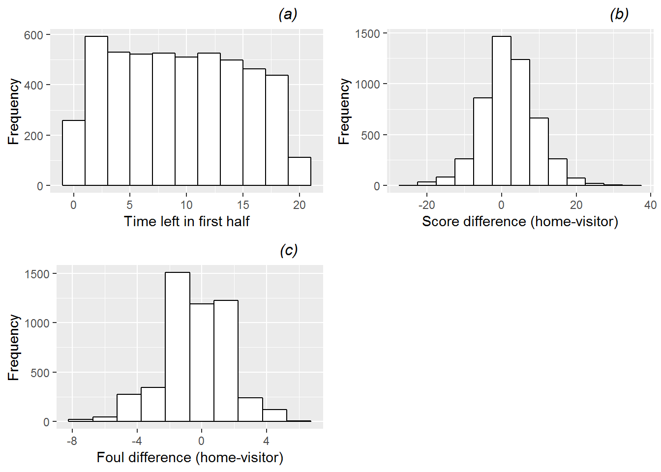
Histograms showing distributions of the 3 continuous Level One covariates: (a) time remaining, (b) score difference, and (c) foul difference.

Figure 11.1: Histograms showing distributions of the 3 continuous Level One covariates: (a) time remaining, (b) score difference, and (c) foul difference.

Summaries of the categorical response (whether the foul was called on the home team) and categorical Level One covariates (whether the home team has the lead and what type of foul was called) can be provided through tables of proportions. More fouls are called on visiting teams (52.1%) than home teams, the home team is more likely to hold a lead (57.1%), and personal fouls are most likely to be called (51.6%), followed by shooting fouls (38.7%) and then offensive fouls (9.7%).

For an initial examination of Level Two covariates (the home and visiting teams), we can take the number of times, for instance, Minnesota (MN) appears in the long data set (with one row per foul called as illustrated in Table 11.1) as the home team and divide by the number of unique games in which Minnesota is the home team. This ratio (12.1), found in Table 11.2, shows that Minnesota is among the bottom three teams in the average total number of fouls in the first halves of games in which it is the home team. That is, games at Minnesota have few total fouls relative to games played elsewhere. Accounting for the effect of home and visiting team will likely be an important part of our model, since some teams tend to play in games with twice as many fouls called as others, and other teams see a noticeable disparity in the total number of fouls depending on if they are home or away.

Table 11.2: Average total number of fouls in the first half over all games in which a particular team is home or visitor. The left columns show the top 3 and bottom 3 teams according to total number of fouls (on both teams) in first halves of games in which they are the home team. The middle columns correspond to games in which the listed teams are the visitors, and the right columns show the largest differences (in both directions) between total fouls in games in which a team is home or visitor.
	Home		Visitor		Difference

	Duke	20.0	WVa	21.4	Duke	4.0
Top 3	VaTech	19.4	Nova	19.0	Wisc	2.6
	Nova	19.1	Wake	18.6	Pitt	2.3

	Mich	10.6	Wisc	10.4	WVa	-6.9
Bottom 3	Ill	11.6	Mich	11.1	Mia	-2.7
	MN	12.1	PSU	11.3	Clem	-2.6

Next, we inspect numerical and graphical summaries of relationships between Level One model covariates and our binary model response. As with other multilevel analyses, we will begin by observing broad trends involving all 4972 fouls called, even though fouls from the same game may be correlated. The conditional density plots in the first row of Figure 11.2 examine continuous Level One covariates. Figure 11.2a provides support for our primary hypothesis about evening out foul calls, indicating a very strong trend for fouls to be more often called on the home team at points in the game when more fouls had previously been called on the visiting team. Figures 11.2b and 11.2c then show that fouls were somewhat more likely to be called on the home team when the home team’s lead was greater and (very slightly) later in the half. Conclusions from the conditional density plots in Figure 11.2a-c are supported with associated empirical logit plots in Figure 11.2d-f. If a logistic link function is appropriate, these plots should be linear, and the stronger the linear association, the more promising the predictor. We see in Figure 11.2d further confirmation of our primary hypothesis, with lower log-odds of a foul called on the home team the greater number of previous fouls the home team had accumulated compared to the visiting team. Figure 11.2e shows that game score may play a role in foul trends, as the log-odds of a foul on the home team grows as the home team accumulates a bigger lead on the scoreboard, and Figure 11.2f shows a very slight tendency for greater log-odds of a foul called on the home team as the half proceeds (since points on the right are closer to the beginning of the game).

Conclusions about continuous Level One covariates are further supported by summary statistics calculated separately for fouls called on the home team and those called on the visiting team. For instance, when a foul is called on the home team, there is an average of 0.64 additional fouls on the visitors at that point in the game, compared to an average of 0.10 additional fouls on the visitors when a foul is called on the visiting team. Similarly, when a foul is called on the home team, they are in the lead by an average of 2.7 points, compared to an average home lead of 1.4 points when a foul is called on the visiting team. As expected, the average time remaining the half is very similar for home and visitor fouls (9.2 vs. 9.5 minutes, respectively).

The mosaic plots in Figure 11.3 examine categorical Level One covariates, indicating that fouls were more likely to be called on the home team when the home team was leading, when the previous foul was on the visiting team, and when the foul was a personal foul rather than a shooting foul or an offensive foul. 51.8% of calls go against the home team when it is leading the game, compared to only 42.9% of calls when the it is behind; 51.3% of calls go against the home team when the previous foul went against the visitors, compared to only 43.8% of calls when the previous foul went against the home team; and, 49.2% of personal fouls are called against the home team, compared to only 46.9% of shooting fouls and 45.7% of offensive fouls. Eventually we will want to examine the relationship between foul type (personal, shooting, or offensive) and foul differential, examining our hypothesis that the tendency to even out calls will be even stronger for calls over which the referees have greater control (personal fouls and especially offensive fouls).

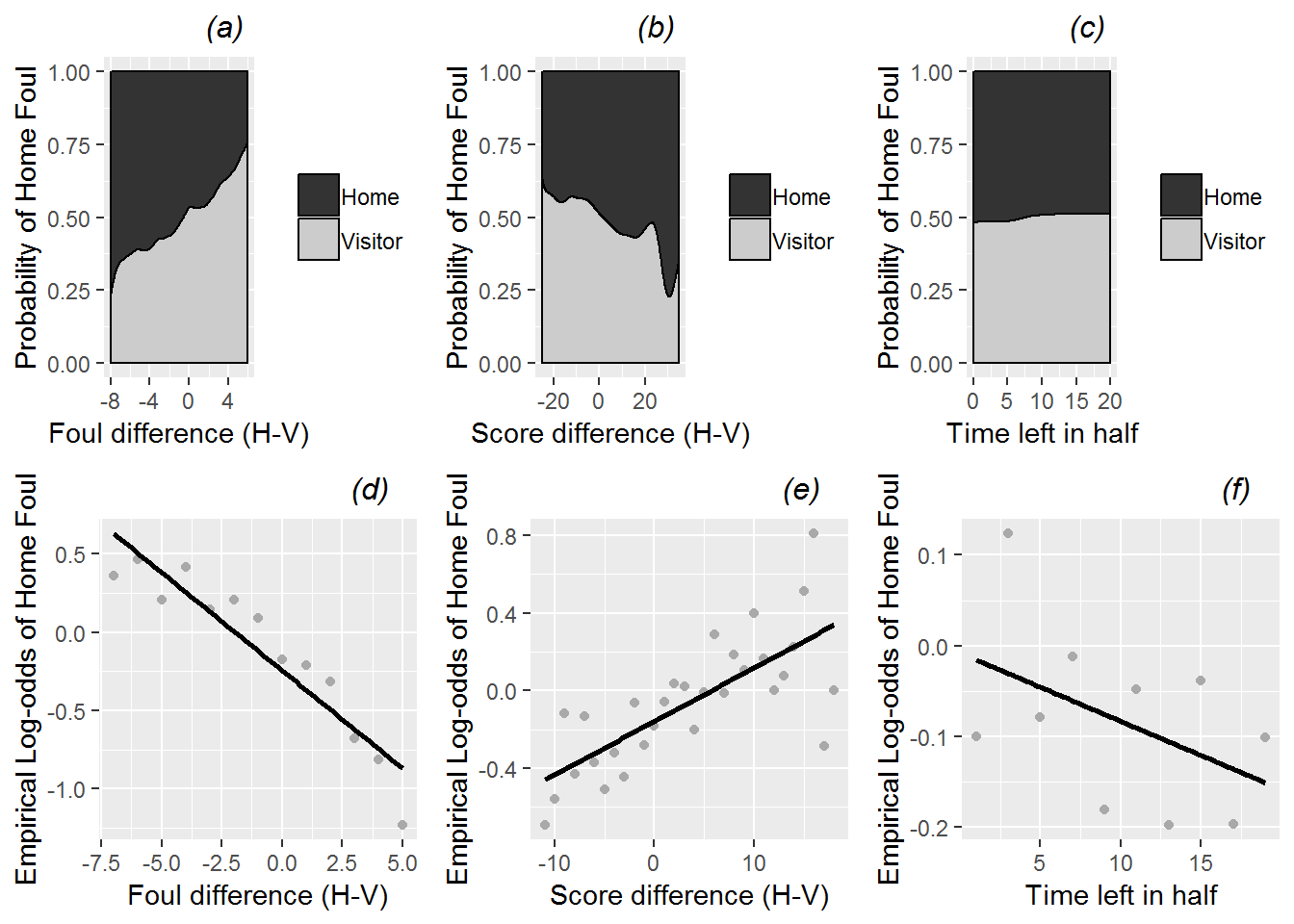
Conditional density and empirical logit plots of the binary model response (foul called on home or visitor) vs. the three continuous Level One covariates (foul differential, score differential, and time remaining). The dark shading in a conditional density plot shows the proportion of fouls called on the home team for a fixed value of (a) foul differential, (b) score differential, and (c) time remaining. In empirical logit plots, estimated log odds of a home team foul are calculated for each distinct foul (d) and score (e) differential, except for differentials at the high and low extremes with insufficient data; for time (f), estimated log odds are calculated for two-minute time intervals and plotted against the midpoints of those interval.

Figure 11.2: Conditional density and empirical logit plots of the binary model response (foul called on home or visitor) vs. the three continuous Level One covariates (foul differential, score differential, and time remaining). The dark shading in a conditional density plot shows the proportion of fouls called on the home team for a fixed value of (a) foul differential, (b) score differential, and (c) time remaining. In empirical logit plots, estimated log odds of a home team foul are calculated for each distinct foul (d) and score (e) differential, except for differentials at the high and low extremes with insufficient data; for time (f), estimated log odds are calculated for two-minute time intervals and plotted against the midpoints of those interval.

Mosaic plots of the binary model response (foul called on home or visitor) vs. the three categorical Level One covariates (foul type (a), team in the lead (b), and team called for the previous foul (c) ). Each bar shows the percentage of fouls called on the home team vs. the percentage of fouls called on the visiting team for a particular category of the covariate. The bar width shows the proportion of fouls at each of the covariate levels.

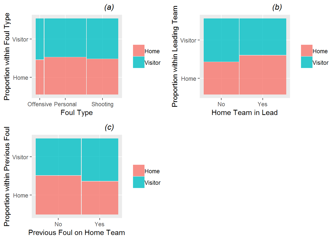
Figure 11.3: Mosaic plots of the binary model response (foul called on home or visitor) vs. the three categorical Level One covariates (foul type (a), team in the lead (b), and team called for the previous foul (c) ). Each bar shows the percentage of fouls called on the home team vs. the percentage of fouls called on the visiting team for a particular category of the covariate. The bar width shows the proportion of fouls at each of the covariate levels.

The exploratory analyses presented above are an essential first step in understanding our data, seeing univariate trends, and noting bivariate relationships between variable pairs. However, our important research questions (a) involve the effect of foul differential after adjusting for other significant predictors of which team is called for a foul, (b) account for potential correlation between foul calls within a game (or within a particular home or visiting team), and (c) determine if the effect of foul differential is constant across game conditions. In order to address research questions such as these, we need to consider multilevel, multivariate statistical models for a binary response variable.

11.4 Two level Modeling with a Generalized Response

11.4.1 A GLM approach (correlation not accounted for)

One quick and dirty approach to analysis might be to run a multiple logistic regression model on the entire long data set of 4972 fouls. In fact, Anderson and Pierce ran such a model in their 2009 paper, using the results of their multiple logistic regression model to support their primary conclusions, while justifying their approach by confirming a low level of correlation within games and the minimal impact on fixed effect estimates that accounting for clustering would have. Output from one potential multiple logistic regression model is shown below; this initial modeling attempt shows significant evidence that referees tend to even out calls (i.e., that the probability of a foul called on the home team decreases as total home fouls increase compared to total visiting team fouls—that is, as foul.diff increases) after accounting for score differential and time remaining (Z=-3.078, p=.002). The extent of the effect of foul differential also appears to grow (in a negative direction) as the first half goes on, based on an interaction between time remaining and foul differential (Z=-2.485, p=.013). We will compare this model with others that formally account for clustering and correlation patterns in our data.

glm(formula = foul.home ~ foul.diff + score.diff + lead.home + 
    time + foul.diff:time + lead.home:time, family = binomial, 
    data = refdata)

Coefficients:
                Estimate Std. Error z value Pr(>|z|)   
(Intercept)    -0.103416   0.101056  -1.023  0.30614   
foul.diff      -0.076599   0.024888  -3.078  0.00209 **
score.diff      0.020062   0.006660   3.012  0.00259 **
lead.home      -0.093227   0.160082  -0.582  0.56032   
time           -0.013141   0.007948  -1.653  0.09827 . 
foul.diff:time -0.007492   0.003014  -2.485  0.01294 * 
lead.home:time  0.021837   0.011161   1.957  0.05040 . 
---
    Null deviance: 6884.3  on 4971  degrees of freedom
Residual deviance: 6747.6  on 4965  degrees of freedom
AIC: 6761.6

11.4.2 A two-stage modeling approach (provides the basic idea for multilevel modeling)

As we saw in Section 8.4.2, to avoid clustering we could consider fitting a separate regression model to each unit of observation at Level Two (each game in this case). Since our primary response variable is binary (Was the foul called on the home team or not?), we would fit a logistic regression model to the data from each game. For example, consider the 14 fouls called during the first half of the March 3, 2010, game featuring Virginia at Boston College (Game 110).

Table 11.3: Key variables from the March 3, 2010, game featuring Virginia at Boston College (Game 110).
visitor	hometeam	foul.num	foul.home	foul.diff	score.diff	foul.type	time
VA	BC	1	0	0	0	Shooting	19.783333
VA	BC	2	0	-1	4	Personal	18.950000
VA	BC	3	0	-2	7	Shooting	16.916667
VA	BC	4	0	-3	10	Personal	14.883333
VA	BC	5	1	-4	10	Personal	14.600000
VA	BC	6	1	-3	6	Offensive	9.750000
VA	BC	7	1	-2	4	Shooting	9.366667
VA	BC	8	0	-1	4	Personal	9.200000
VA	BC	9	0	-2	6	Shooting	7.666667
VA	BC	10	0	-3	12	Shooting	2.500000
VA	BC	11	1	-4	13	Personal	2.083333
VA	BC	12	1	-3	13	Personal	1.966667
VA	BC	13	0	-2	12	Shooting	1.733333
VA	BC	14	1	-3	14	Personal	0.700000

Is there evidence from this game that referees tend to “even out” foul calls when one team starts to accumulate more fouls? Is the score differential associated with the probability of a foul on the home team? Is the effect of foul differential constant across all foul types during this game? We can address these questions through multiple logistic regression applied to only data from Game 110.

First, notation must be defined. Let \(Y_{ij}\) be an indicator variable recording if the \(j^{th}\) foul from Game \(i\) was called on the home team (1) or the visiting team (0). We can consider \(Y_{ij}\) to be a Bernoulli random variable with parameter \(p_{ij}\), where \(p_{ij}\) is the true probability that the \(j^{th}\) foul from Game \(i\) was called on the home team. As in Chapter 6, we will begin by modeling the logit function of \(p_{ij}\) for Game \(i\) as a linear function of Level One covariates. For instance, if we were to consider a simple model with foul differential as the sole predictor, we could model the probability of a foul on the home team in Game 110 with the model: \[\begin{equation} \log\bigg(\frac{p_{110j}}{1-p_{110j}}\bigg)=a_{110}+b_{110}\mathrm{foul.diff}_{110j} \tag{11.1} \end{equation}\]

where \(i\) is fixed at 110. Note that there is no separate error term or variance parameter, since the variance is a function of \(p_{ij}\) with a Bernoulli random variable.

Maximum likelihood estimators for the parameters in this model (\(a_{110}\) and \(b_{110}\)) can be obtained through statistical software. \(e^{a_{110}}\) represents the odds that a foul is called on the home team when the foul totals in Game 110 are even, and \(e^{b_{110}}\) represents the multiplicative change in the odds that a foul is called on the home team for each additional foul for the home team relative to the visiting team during the first half of Game 110. For example, if we compared the situation when the home team has been called for 3 more fouls than the visiting team to when the home team has been called for 4 more fouls than the visitors, we’d estimate \(e^{b_{110}}\) to be the multiplicative difference in odds of a foul called on the home team (the odds should decrease from 3 to 4 additional home fouls).

For Game 110, we estimate \(\hat{a}_{110}=-5.67\) and \(\hat{b}_{110}=-2.11\) (see output below). Thus, according to our simple logistic regression model, the odds that a foul is called on the home team when both teams have an equal number of fouls in Game 110 is \(e^{-5.67}=0.0035\); that is, the probability that a foul is called on the visiting team (0.9966) is \(1/0.0035 = 289\) times higher than the probability a foul is called on the home team (0.0034) in that situation. While these parameter estimates seem quite extreme, reliable estimates are difficult to obtain with 14 observations and a binary response variable, especially in a case like this where the fouls were only even at the start of the game. Also, as the gap between home and visiting fouls increases by 1, the odds that a foul is called on the visiting team increases by a multiplicative factor of more than 8 (since \(1/e^{-2.11}=8.25\)). In Game 110, this trend toward referees evening out foul calls is statistically significant at the 0.10 level (Z=-1.851, p=.0642).

glm(formula = foul.home ~ foul.diff, family = binomial, data = game110)

Coefficients:
            Estimate Std. Error z value Pr(>|z|)  
(Intercept)   -5.668      3.131  -1.810   0.0703 .
foul.diff     -2.110      1.140  -1.851   0.0642 .
---
    Null deviance: 19.121  on 13  degrees of freedom
Residual deviance: 11.754  on 12  degrees of freedom
AIC: 15.754

As in Section 8.4.2, we can proceed to fit similar logistic regression models for each of the 339 other games in our data set. Each model will yield a new estimate of the intercept and the slope from Equation (11.1). These estimates are summarized graphically in Figure 11.4. There is noticeable variability among the 340 games in the fitted intercepts and slopes, with an IQR for intercepts ranging from -1.45 to 0.70, and an IQR for slopes ranging from -1.81 to -0.51. The majority of intercepts are below 0 (median = -0.41), so that in most games a foul is less likely to be called on the home team when foul totals are even. In addition, almost all of the estimated slopes are below 0 (median = -0.89), indicating that as the home team’s foul total grows in relation to the visiting team’s foul total, the odds of a foul on the home team continues to decrease.

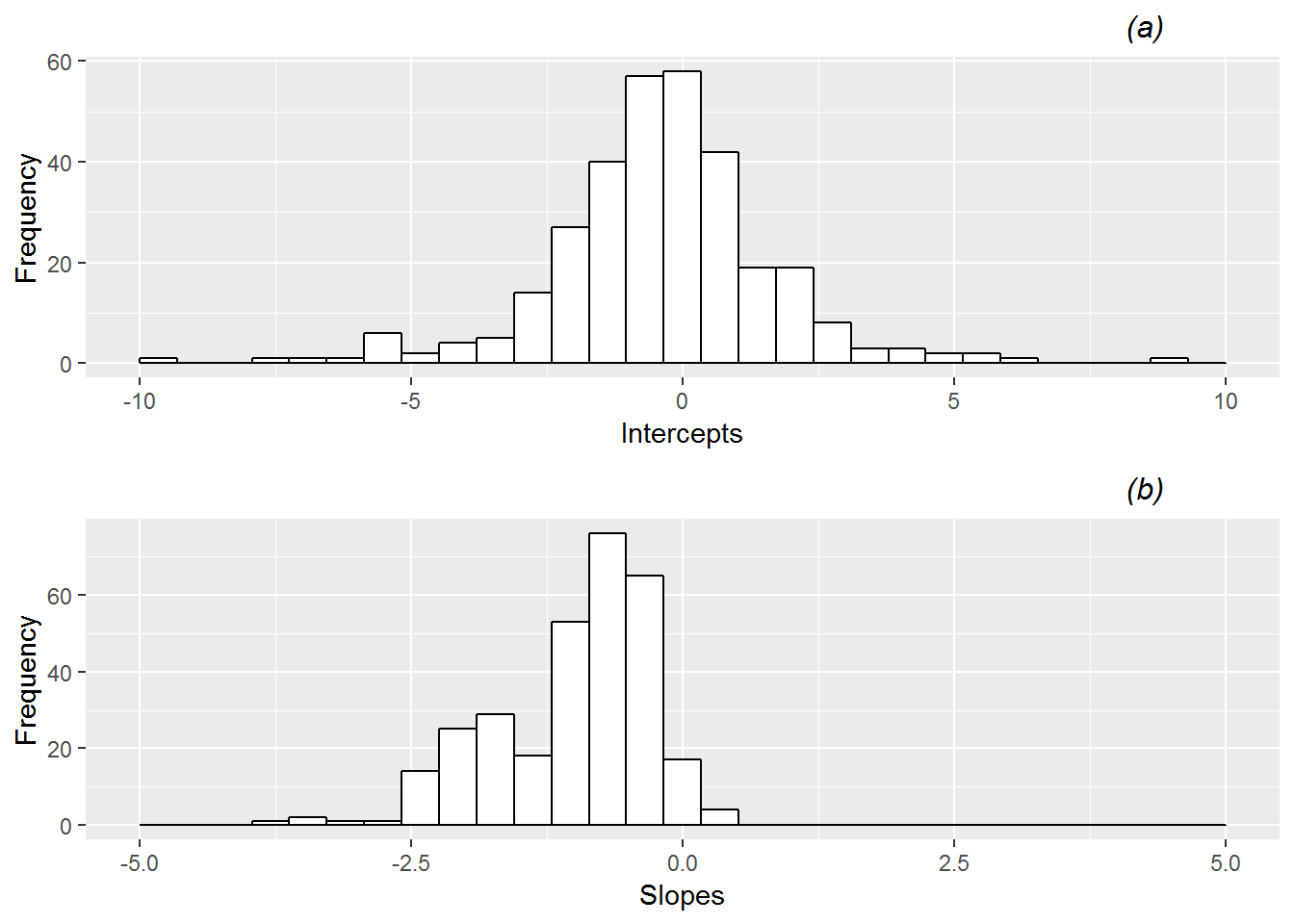
Histograms of (a) intercepts and (b) slopes from fitting simple logistic regression models by game. Several extreme outliers have been cut off in these plots for illustration purposes.

Figure 11.4: Histograms of (a) intercepts and (b) slopes from fitting simple logistic regression models by game. Several extreme outliers have been cut off in these plots for illustration purposes.

At this point, you might imagine expanding model building efforts in a couple of directions: (a) continue to improve the Level One model in Equation (11.1) by controlling for covariates and adding potential interaction terms, or (b) build Level Two models to explain the game-to-game variability in intercepts or slopes using covariates which remain constant from foul to foul within a game (like the teams playing). While we could pursue these two directions independently, we can accomplish our modeling goals in a much cleaner and more powerful way by proceeding as in Chapter 8 and building a unified multilevel framework under which all parameters are estimated simultaneously and we remain faithful to the correlation structure inherent in our data.

11.4.3 A unified multilevel approach (the framework we’ll use)

As in Chapters 8 and 9, we will write out a composite model after first expressing Level One and Level Two models. That is, we will create Level One and Level Two models as in Section 11.4.2, but we will then combine those models into a composite model and estimate all model parameters simultaneously. Once again \(Y_{ij}\) is an indicator variable recording if the \(j^{th}\) foul from Game \(i\) was called on the home team (1) or the visiting team (0), and \(p_{ij}\) is the true probability that the \(j^{th}\) foul from Game \(i\) was called on the home team. Our Level One model with foul differential as the sole predictor is given by Equation (11.1): \[ \log\bigg(\frac{p_{ij}}{1-p_{ij}}\bigg)=a_i+b_i\mathrm{foul.diff}_{ij} \] Then we include no fixed covariates at Level Two, but we include error terms to allow the intercept and slope from Level One to vary by game, and we allow these errors to be correlated:

\[\begin{eqnarray*} a_i & = & \alpha_{0}+u_i \\ b_i & = & \beta_{0}+v_i, \end{eqnarray*}\]

where the error terms at Level Two can be assumed to follow a multivariate normal distribution:

\[ \left[ \begin{array}{c} a_i \\ b_i \end{array} \right] \sim N \left( \left[ \begin{array}{c} 0 \\ 0 \end{array} \right], \left[ \begin{array}{cc} \sigma_{u}^{2} & \\ \sigma_{uv} & \sigma_{v}^{2} \end{array} \right] \right) \]

Our composite model then looks like:

\[\begin{eqnarray*} \log\bigg(\frac{p_{ij}}{1-p_{ij}}\bigg) & = & a_i+b_i\mathrm{foul.diff}_{ij} \\ & = & (\alpha_{0}+u_i) + (\beta_{0}+v_i)\mathrm{foul.diff}_{ij} \\ & = & [\alpha_{0}+\beta_{0}\mathrm{foul.diff}_{ij}]+[u_i+v_i\mathrm{foul.diff}_{ij}] \end{eqnarray*}\]

The major changes when moving from a normally distributed response to a binary response are the form of the response variable (a logit function) and the absence of an error term at Level One.

Again, we can use statistical software to obtain parameter estimates for this unified multilevel model using all 4972 fouls recorded from the 340 games. For example, the glmer() function from the lme4 package in R extends the lmer() function to handle generalized responses and to account for the fact that fouls are not independent within games. Results are given below for the two-level model with foul differential as the sole covariate and Game as the Level Two observational unit.

Formula: foul.home ~ foul.diff + (foul.diff | game)

     AIC      BIC   logLik deviance df.resid 
  6791.1   6823.6  -3390.5   6781.1     4967 

Random effects:
 Groups Name        Variance Std.Dev. Corr 
 game   (Intercept) 0.294141 0.54235       
        foul.diff   0.001235 0.03514  -1.00
Number of obs: 4972, groups:  game, 340

Fixed effects:
            Estimate Std. Error z value Pr(>|z|)    
(Intercept) -0.15684    0.04637  -3.382 0.000719 ***
foul.diff   -0.28532    0.03835  -7.440 1.01e-13 ***

When parameter estimates from the multilevel model above are compared with those from the naive logistic regression model assuming independence of all observations (below), there are noticeable differences. For instance, each additional foul for the visiting team is associated with a 33% increase (\(1/e^{-.285}\)) in the odds of a foul called on the home team under the multilevel model, but the single level model estimates the same increase as only 14% (\(1/e^{-.130}\)). Also, estimated standard errors for fixed effects are greater under generalized linear multilevel modeling, which is not unusual after accounting for correlated observations, which effectively reduces the sample size.

glm(formula = foul.home ~ foul.diff, family = binomial, data = refdata)

Coefficients:
            Estimate Std. Error z value Pr(>|z|)    
(Intercept) -0.13005    0.02912  -4.466 7.98e-06 ***
foul.diff   -0.13047    0.01426  -9.148  < 2e-16 ***
---
    Null deviance: 6884.3  on 4971  degrees of freedom
Residual deviance: 6798.1  on 4970  degrees of freedom
AIC: 6802.1

11.5 Crossed Random Effects

In the College Basketball Referees case study, our two primary Level Two covariates are home team and visiting team. In Section 11.3.2 we showed evidence that the probability a foul is called on the home team changes if we know precisely who the home and visiting teams are. However, if we were to include an indicator variable for each distinct team, we would need 38 indicator variables for home teams and 38 more for visiting teams. That’s a lot of degrees of freedom to spend! And adding those indicator variables would complicate our model considerably, despite the fact that we’re not very interested in specific coefficient estimates for each team—we just want to control for teams playing to draw stronger conclusions about referee bias (focusing on the foul.diff variable). One way, then, of accounting for teams is by treating them as random effects rather than fixed effects. For instance, we can assume the effect that Minnesota being the home team has on the log odds of foul call on the home team is drawn from a normal distribution with mean 0 and variance \(\sigma^{2}_{v}\). Maybe the estimated random effect for Minnesota as the home team is -0.5, so that Minnesota is slightly less likely that the typical home team to have fouls called on it, and the odds of a foul on the home team are somewhat correlated whenever Minnesota is the home team. In this way, we account for the complete range of team effects, while only having to estimate a single parameter (\(\sigma^{2}_{v}\)) rather than coefficients for 38 indicator variables. The effect of visiting teams can be similarly modeled.

How will treating home and visiting teams as random effects change our multilevel model? Another way we might view this situation is by considering that Game is not the only Level Two observational unit we might have selected. What if we instead decided to focus on Home Team as the Level Two observational unit? That is, what if we assumed that fouls called on the same home team across all games must be correlated? In this case, we could redefine our Level One model from Equation (11.1). Let \(Y_{hj}\) be an indicator variable recording if the \(j^{th}\) foul from Home Team \(h\) was called on the home team (1) or the visiting team (0), and \(p_{hj}\) be the true probability that the \(j^{th}\) foul from Home Team \(h\) was called on the home team. Now, if we were to consider a simple model with foul differential as the sole predictor, we could model the probability of a foul on the home team for Home Team \(h\) with the model:

\[\begin{equation} \log\bigg(\frac{p_{hj}}{1-p_{hj}}\bigg)=a_h+b_h\mathrm{foul.diff}_{hj} \tag{11.2} \end{equation}\]

In this case, \(e^{a_{h}}\) represents the odds that a foul is called on the home team when total fouls are equal between both teams in a game involving Home Team \(h\), and \(e^{b_{h}}\) represents the multiplicative change in the odds that a foul is called on the home team for every extra foul on the home team compared to the visitors in a game involving Home Team \(h\). After fitting logistic regression models for each of the 39 teams in our data set, we see in Figure 11.5 variability in fitted intercepts (mean=-0.15, sd=0.33) and slopes (mean=-0.22, sd=0.12) among the 39 teams, although much less variability than we observed from game-to-game. Of course, each logistic regression model for a home team was based on about 10 times more foul calls than each model for a game, so observing less variability from team-to-team was not unexpected.

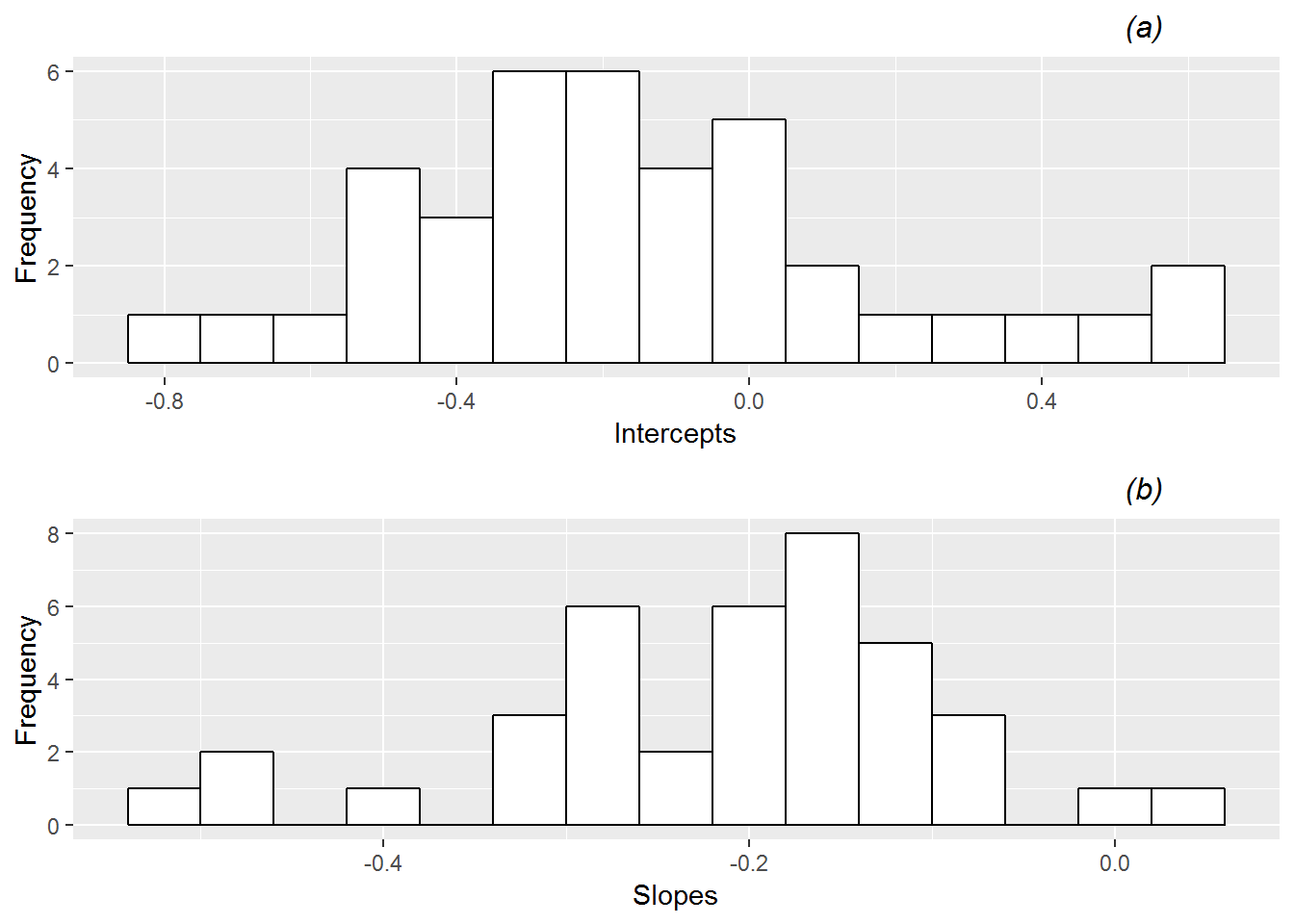
Figure 11.5: Histograms of (a) intercepts and (b) slopes from fitting simple logistic regression models by home team.

From a modeling perspective, accounting for clustering by game and by home team (not to mention by visiting team) brings up an interesting issue we have not yet considered—can we handle random effects that are not nested? Since each foul called is associated with only one game (or only one home team and one visiting team), foul is considered nested in game (or home or visiting team). However, a specific home team is not associated with a single game; that home team appears in several games. Therefore, any effects of game, home team, and visiting team are considered crossed random effects.

A two-level model which accounts for variability among games, home teams, and visiting teams would take on a slightly new look. First, the full subscripting would change a bit. Our primary response variable would now be written as \(Y_{i[gh]j}\), an indicator variable recording if the \(j^{th}\) foul from Game \(i\) was called on the home team (1) or the visiting team (0), where Game \(i\) pitted Visiting Team \(g\) against Home Team \(h\). Square brackets are introduced since \(g\) and \(h\) are essentially at the same level as \(i\), whereas we have assumed (without stating so) throughout this book that subscripting without square brackets implies a movement to lower levels as the subscripts move left to right (e.g., \(ij\) indicates \(i\) units are at Level Two, while \(j\) units are at Level One, nested inside Level Two units). We can then consider \(Y_{i[gh]j}\) to be a Bernoulli random variable with parameter \(p_{i[gh]j}\), where \(p_{i[gh]j}\) is the true probability that the \(j^{th}\) foul from Game \(i\) was called on Home Team \(h\) rather than Visiting Team \(g\). We will include the crossed subscripting only where necessary.

Typically, with the addition of crossed effects, the Level One model will remain familiar and changes will be seen at Level Two, especially in the equation for the intercept term. In the model formulation below we allow, as before, the slope and intercept to vary by game:

Level One: \[\begin{equation} \log\bigg(\frac{p_{i[gh]j}}{1-p_{i[gh]j}}\bigg)=a_{i}+b_{i}\mathrm{foul.diff}_{ij} \tag{11.3} \end{equation}\]
Level Two: \[\begin{eqnarray*} a_{i} & = & \alpha_{0}+u_{i}+v_{h}+w_{g} \\ b_{i} & = & \beta_{0}, \end{eqnarray*}\]

Therefore, at Level Two, we assume that \(a_{i}\), the log odds of a foul on the home team when the home and visiting teams in Game \(i\) have an equal number of fouls, depends on four components:

\(\alpha_{0}\) is the population average log odds across all games and fouls (fixed)
\(u_{i}\) is the effect of Game \(i\) (random)
\(v_{h}\) is the effect of Home Team \(h\) (random)
\(w_{g}\) is the effect of Visiting Team \(g\) (random)

where error terms (random effects) at Level Two can be assumed to follow independent normal distributions: \[\begin{eqnarray*} u_{i} & \sim & N \left( 0 , \sigma_{u}^{2} \right) \\ v_{h} & \sim & N \left( 0 , \sigma_{v}^{2} \right) \\ w_{g} & \sim & N \left( 0 , \sigma_{w}^{2} \right). \end{eqnarray*}\]

We could include terms that vary by home or visiting team in other Level Two equations, but often adjusting for these random effects on the intercept is sufficient. The advantages to including additional random effects are three-fold. First, by accounting for additional sources of variability, we should obtain more precise estimate of other model parameters, including key fixed effects. Second, we obtain estimates of variance components, allowing us to compare the relative sizes of game-to-game and team-to-team variability. Third, as outlined in Section 11.8, we can obtain estimated random effects which allow us to compare the effects on the log-odds of a home foul of individual home and visiting teams.

Our composite model then looks like: \[\begin{equation} \log\bigg(\frac{p_{i[gh]j}}{1-p_{i[gh]j}}\bigg) = [\alpha_{0}+\beta_{0}\mathrm{foul.diff}_{ij}]+[u_{i}+v_{h}+w_{g}]. \tag{11.4} \end{equation}\]

We will refer to this as Model A, where we look at the effect of foul differential on the odds a foul is called on the home team, while accounting for three crossed random effects at Level Two (game, home team, and visiting team). Parameter estimates for Model A are given below:

Formula: 
   Data: refdata

     AIC      BIC   logLik deviance df.resid 
  6780.5   6813.0  -3385.2   6770.5     4967 

Random effects:
 Groups   Name        Variance Std.Dev.
 game     (Intercept) 0.17164  0.4143  
 hometeam (Intercept) 0.06809  0.2609  
 visitor  (Intercept) 0.02323  0.1524  
Number of obs: 4972, groups:  game, 340; hometeam, 39; visitor, 39

Fixed effects:
            Estimate Std. Error z value Pr(>|z|)    
(Intercept) -0.18780    0.06331  -2.967  0.00301 **

From this output, we obtain estimates of our five model parameters:

\(\hat{\alpha}_{0}=-0.188=\) the mean log odds of a home foul at the point where total fouls are equal between teams. In other words, when fouls are balanced between teams, the odds that a foul is called on the visiting team is 20.7% higher than the odds a foul is called on the home team (\(1/e^{-.188}=1.207\)).
\(\hat{\beta}_{0}=-0.264=\) the decrease in mean log odds of a home foul for each 1 foul increase in the foul differential. More specifically, the odds the next foul is called on the visiting team rather than the home team increases by 30.2% with each additional foul called on the home team (\(1/e^{-.264}=1.302\)).
\(\hat{\sigma}_{u}^{2}=0.172=\) the variance in intercepts from game-to-game.
\(\hat{\sigma}_{v}^{2}=0.068=\) the variance in intercepts among different home teams.
\(\hat{\sigma}_{w}^{2}=0.023=\) the variance in intercepts among different visiting teams.

Based on the t-value (-6.80) and p-value (\(p<.001\)) associated with foul differential in this model, we have significant evidence of a negative association between foul differential and the odds of a home team foul. That is, we have significant evidence that the odds that a foul is called on the home team shrinks as the home team has more total fouls compared with the visiting team. Thus, there seems to be preliminary evidence in the 2009-10 data that college basketball referees tend to even out foul calls over the course of the first half. Of course, we have yet to adjust for other significant covariates.

11.6 Model Comparisons Using the Parametric Bootstrap

Our estimates of variance components provide evidence of the relative variability in the different Level Two random effects. For example, an estimated 65.4% of variability in the intercepts is due to differences from game-to-game, while 25.9% is due to differences among home teams, and 8.7% is due to differences among visiting teams. At this point, we could reasonably ask: if we use a random effect to account for differences among games, does it really pay off to also account for which team is home and which is the visitor?

To answer this, we could compare models with and without the random effects for home and visiting teams (i.e., Model A, the full model, vs. Model A.0, the reduced model) using a likelihood ratio test. In Model A.0, Level Two now looks like: \[\begin{eqnarray*} a_{i} & = & \alpha_{0}+u_{i} \\ b_{i} & = & \beta_{0}, \end{eqnarray*}\]

The likelihood ratio test (see below) provides significant evidence (LRT=16.074, df=2, p=.0003) that accounting for variability among home teams and among visiting teams improves our model.

Data: refdata
Models:
model.0a: foul.home ~ foul.diff + (1 | game)
model.a: foul.home ~ foul.diff + (1 | game) + (1 | hometeam) + (1 | visitor)
         Df    AIC    BIC  logLik deviance  Chisq Chi Df Pr(>Chisq)    
model.0a  3 6792.5 6812.1 -3393.3   6786.5                             
model.a   5 6780.5 6813.0 -3385.2   6770.5 16.074      2  0.0003233 ***
---
Signif. codes:  0 '***' 0.001 '**' 0.01 '*' 0.05 '.' 0.1 ' ' 1

In Section 8.5.4 we noted that REML estimation is typically used when comparing models that differ only in random effects for multilevel models with normal responses, but with generalized linear multilevel models, full maximum likelihood (ML) estimation procedures are typically used regardless of the situation (including in the function glmer() in R). So the likelihood ratio test above is based on ML methods—can we trust its accuracy? In Section 10.6 we introduced the parametric bootstrap as a more reliable method in many cases for conducting hypothesis tests compared to the likelihood ratio test, especially when comparing full and reduced models that differ in their variance components. What would a parametric bootstrap test say about testing \(H_{0}: \sigma_{v}^{2}=\sigma_{w}^{2}=0\) vs. \(H_{A}:\) at least one of \(\sigma_{v}^{2}\) or \(\sigma_{w}^{2}\) is not equal to 0? Under the null hypothesis, since the two variance terms are being set to a value (0) on the boundary constraint, we would not expect the chi-square distribution to adequately approximate the behavior of the likelihood ratio test statistic.

Figure 11.6 illustrates the null distribution of the likelihood ratio test statistic derived by the parametric bootstrap procedure with 100 samples as compared to a chi-square distribution. As we observed in Section 10.6, the parametric bootstrap provides a more reliable p-value in this case (\(p<.001\) from output below) because a chi-square distribution puts too much mass in the tail and not enough near 0. However, the parametric bootstrap is computationally intensive, and it can take a long time to run even with moderately complex models. With this data, we would select our full Model A based on a parametric bootstrap test.

## Data: refdata
## Parametric bootstrap with 100 samples.
## Models:
## m0: foul.home ~ foul.diff + (1 | game)
## mA: foul.home ~ foul.diff + (1 | game) + (1 | hometeam) + (1 | visitor)
##    Df    AIC    BIC  logLik deviance  Chisq Chi Df Pr_boot(>Chisq)
## m0  3 6792.5 6812.1 -3393.3   6786.5                              
## mA  5 6780.5 6813.0 -3385.2   6770.5 16.074      2               0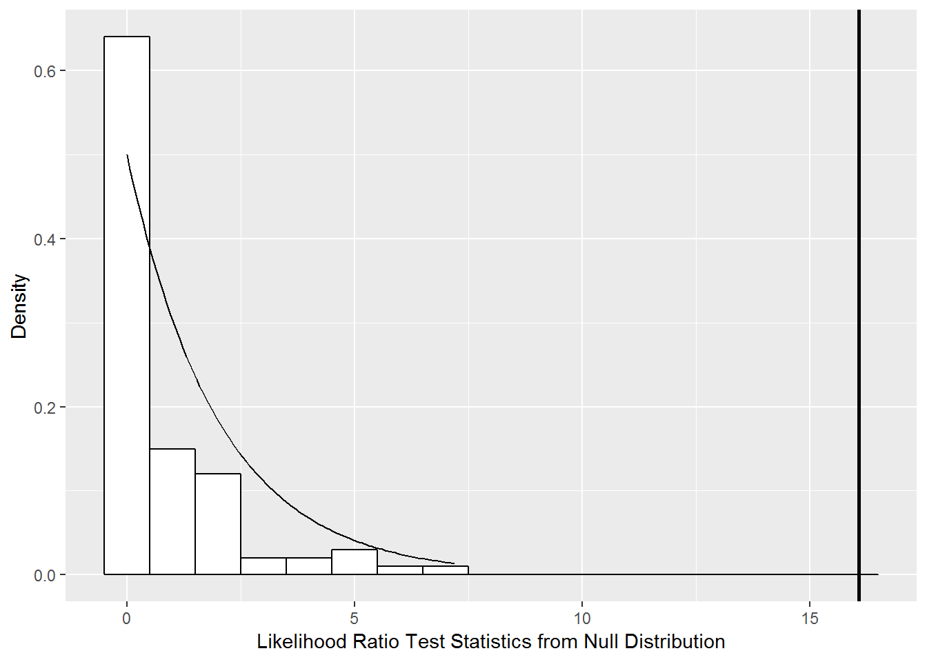

Null distribution of likelihood ratio test statistic comparing Models A and A.0 derived using parametric bootstrap with 100 samples (histogram) compared to a chi-square distribution with 2 degrees of freedom (smooth curve).

Figure 11.6: Null distribution of likelihood ratio test statistic comparing Models A and A.0 derived using parametric bootstrap with 100 samples (histogram) compared to a chi-square distribution with 2 degrees of freedom (smooth curve).

We might also reasonably ask: is it helpful to allow slopes (coefficients for foul differential) to vary by game, home team, and visiting team as well? Again, since we are comparing models that differ in random effects, and since the null hypothesis involves setting random effects at their boundaries, we use the parametric bootstrap. Formally, we are comparing Model A to Model A.1, which has the same Level One equation as Model A: \[ \log\bigg(\frac{p_{i[gh]j}}{1-p_{i[gh]j}}\bigg)=a_{i}+b_{i}\mathrm{foul.diff}_{ij} \] but more variance components to estimate at Level Two: \[\begin{eqnarray*} a_{i} & = & \alpha_{0}+u_{i}+v_{h}+w_{g} \\ b_{i} & = & \beta_{0}+z_{i}+r_{h}+s_{g}, \end{eqnarray*}\] where error terms (random effects) at Level Two can be assumed to follow independent normal distributions: \[\begin{eqnarray*} u_{i} & \sim & N \left( 0 , \sigma_{u}^{2} \right) \\ z_{i} & \sim & N \left( 0 , \sigma_{z}^{2} \right) \\ v_{h} & \sim & N \left( 0 , \sigma_{v}^{2} \right) \\ r_{h} & \sim & N \left( 0 , \sigma_{r}^{2} \right) \\ w_{g} & \sim & N \left( 0 , \sigma_{w}^{2} \right) \\ s_{g} & \sim & N \left( 0 , \sigma_{s}^{2} \right). \end{eqnarray*}\]

Thus our null hypothesis for comparing Model A vs. Model A.1 is \(H_{O}: \sigma_{z}^{2}=\sigma_{r}^{2}=\sigma_{s}^{2}=0\). We do not have significant evidence (LRT=0.349, df=3, p=.46 by parametric bootstrap) of variability among slopes, so we will only include random effects for game, home team, and visiting team for the intercept going forward. Figure 11.7 illustrates the null distribution of the likelihood ratio test statistic derived by the parametric bootstrap procedure as compared to a chi-square distribution, again showing that the tails are too heavy in the chi-square distribution.

## Data: refdata
## Parametric bootstrap with 100 samples.
## Models:
## m0: foul.home ~ foul.diff + (1 | game) + (1 | hometeam) + (1 | visitor)
## mA: foul.home ~ foul.diff + (1 | game) + (1 | hometeam) + (1 | visitor) + 
## mA:     (0 + foul.diff | game) + (0 + foul.diff | hometeam) + (0 + 
## mA:     foul.diff | visitor)
##    Df    AIC    BIC  logLik deviance Chisq Chi Df Pr_boot(>Chisq)
## m0  5 6780.5 6813.0 -3385.2   6770.5                             
## mA  8 6786.1 6838.2 -3385.1   6770.1 0.349      3            0.46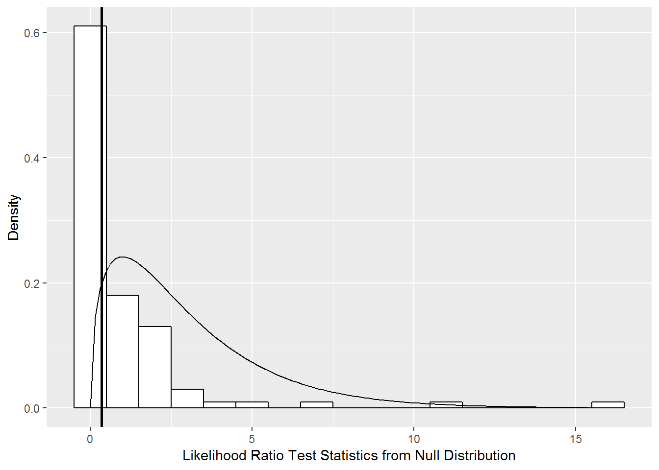

Null distribution of likelihood ratio test statistic comparing Models A and A.1 derived using parametric bootstrap with 100 samples (histogram) compared to a chi-square distribution with 3 degrees of freedom (smooth curve).

Figure 11.7: Null distribution of likelihood ratio test statistic comparing Models A and A.1 derived using parametric bootstrap with 100 samples (histogram) compared to a chi-square distribution with 3 degrees of freedom (smooth curve).

Note that we could have also allowed for a correlation between the error terms for the intercept and slope by game, home team, or visiting team – i.e., assume, for example: \[ \left[ \begin{array}{c} u_{i} \\ z_{i} \end{array} \right] \sim N \left( \left[ \begin{array}{c} 0 \\ 0 \end{array} \right], \left[ \begin{array}{cc} \sigma_{u}^{2} & \\ \sigma_{uz} & \sigma_{z}^{2} \end{array} \right] \right) \] while error terms by game, home team, or visiting team are still independent. Here, the new model would have 6 additional parameters when compared with Model A (3 variance terms and 3 covariance terms). By the parametric bootstrap, there is no significant evidence that the model with 6 additional parameters is necessary (LRT=6.49, df=6, p=.06 by parametric bootstrap). The associated p-value based on a likelihood ratio test with approximate chi-square distribution (and restricted maximum likelihood estimation) is .370, reflecting once again the overly heavy tails of the chi-square distribution.

11.7 A Potential Final Model for Examining Referee Bias

In constructing a final model for this college basketball case study, we are guided by several considerations. First, we want to estimate the effect of foul differential on the odds of a home foul, after adjusting for important covariates. Second, we wish to find important interactions with foul differential, recognizing that the effect of foul differential might depend on the game situation and other covariates. Third, we want to account for random effects associated with game, home team, and visiting team. What follows is one potential final model that follows these guidelines:

Level One: \[\begin{eqnarray*} \log\bigg(\frac{p_{i[gh]j}}{1-p_{i[gh]j}}\bigg) & = & a_{i} + b_{i}\mathrm{foul.diff}_{ij} + c_{i}\mathrm{score.diff}_{ij} + d_{i}\mathrm{lead.home}_{ij} + f_{i}\mathrm{time}_{ij} \\ & &{} + k_{i}\mathrm{offensive}_{ij} + l_{i}\mathrm{personal}_{ij} + m_{i}\mathrm{foul.diff:offensive}_{ij} \\ & &{} + n_{i}\mathrm{foul.diff:personal}_{ij} + o_{i}\mathrm{foul.diff:time}_{ij} \\ & &{} + q_{i}\mathrm{lead.home:time}_{ij} \end{eqnarray*}\]
Level Two: \[\begin{eqnarray*} a_{i} & = & \alpha_{0}+u_{i}+v_{h}+w_{g} \\ b_{i} & = & \beta_{0} \\ c_{i} & = & \gamma_{0} \\ d_{i} & = & \delta_{0} \\ f_{i} & = & \phi_{0} \\ k_{i} & = & \kappa_{0} \\ l_{i} & = & \lambda_{0} \\ m_{i} & = & \mu_{0} \\ n_{i} & = & \nu_{0} \\ o_{i} & = & \omega_{0} \\ q_{i} & = & \xi_{0}, \end{eqnarray*}\]

where error terms at Level Two can be assumed to follow independent normal distributions: \[\begin{eqnarray*} u_{i} & \sim & N \left( 0 , \sigma_{u}^{2} \right) \\ v_{h} & \sim & N \left( 0 , \sigma_{v}^{2} \right) \\ w_{g} & \sim & N \left( 0 , \sigma_{w}^{2} \right). \end{eqnarray*}\] Our composite model then looks like: \[\begin{eqnarray*} \log\bigg(\frac{p_{i[gh]j}}{1-p_{i[gh]j}}\bigg) & = & [\alpha_{0} + \beta_{0}\mathrm{foul.diff}_{ij} + \gamma_{0}\mathrm{score.diff}_{ij} + \delta_{0}\mathrm{lead.home}_{ij} + \phi_{0}\mathrm{time}_{ij} \\ & &{} + \kappa_{0}\mathrm{offensive}_{ij} + \lambda_{0}\mathrm{personal}_{ij} + \mu_{0}\mathrm{foul.diff:offensive}_{ij} \\ & &{} + \nu_{0}\mathrm{foul.diff:personal}_{ij} + \omega_{0}\mathrm{foul.diff:time}_{ij} \\ & &{} + \xi_{0}\mathrm{lead.home:time}_{ij}] + [u_{i}+v_{h}+w_{g}]. \end{eqnarray*}\]

Using the composite form of this generalized linear multilevel model, the parameter estimates for our 11 fixed effects and 3 variance components are given in the output below:

Formula: 
foul.home ~ foul.diff + score.diff + lead.home + time + offensive +  
    personal + foul.diff:offensive + foul.diff:personal + foul.diff:time +  
   Data: refdata

     AIC      BIC   logLik deviance df.resid 
  6731.0   6822.2  -3351.5   6703.0     4958 

Random effects:
 Groups   Name        Variance Std.Dev.
 game     (Intercept) 0.18460  0.4297  
 hometeam (Intercept) 0.07831  0.2798  
 visitor  (Intercept) 0.04313  0.2077  
Number of obs: 4972, groups:  game, 340; hometeam, 39; visitor, 39

Fixed effects:
                     Estimate Std. Error z value Pr(>|z|)    
(Intercept)         -0.246486   0.133961  -1.840 0.065771 .  
foul.diff           -0.171462   0.045364  -3.780 0.000157 ***
score.diff           0.033521   0.008236   4.070  4.7e-05 ***
lead.home           -0.150620   0.177214  -0.850 0.395360    
time                -0.008746   0.008560  -1.022 0.306920    
offensive           -0.080791   0.111234  -0.726 0.467648    
personal             0.067203   0.065397   1.028 0.304132    
foul.diff:offensive -0.103578   0.053869  -1.923 0.054509 .  
foul.diff:personal  -0.055638   0.031948  -1.742 0.081590 .  
foul.diff:time      -0.008689   0.003274  -2.654 0.007953 ** 
lead.home:time       0.026007   0.012172   2.137 0.032624 *

In general, we see a highly significant negative effect of foul differential—a strong tendency for referees to even out foul calls when one team starts amassing more fouls than the other. Important covariates to control for (because of their effects on the odds of a home foul) include score differential, whether the home team held the lead, time left in the first half, and the type of foul called.

Furthermore, we see that the effect of foul differential depends on type of foul called and time left in the half—the tendency for evening out foul calls is stronger earlier in the half, and when offensive and personal fouls are called instead of shooting fouls. The effect of foul type supports the hypothesis that if referees are consciously or subconsciously evening out foul calls, the behavior will be more noticeable for calls over which they have more control, especially offensive fouls (which are notorious judgment calls) and then personal fouls (which don’t affect a player’s shot, and thus a referee can choose to let them go uncalled). Evidence like this can be considered dose response, since higher “doses” of referee control are associated with a greater effect of foul differential on their calls. A dose response effect provides even stronger indication of referee bias.

Analyses of data from 2004-05 (Noecker and Roback 2012) showed that the tendency to even out foul calls was stronger when one team had a large lead, but we found no evidence of a foul differential by score differential interaction in the 2009-10 data, although home team fouls are more likely when the home team has a large lead, regardless of the foul differential.

Here are specific interpretations of key model parameters:

\(\exp(\hat{\alpha}_{0})=\exp(-0.247)=0.781\). The odds of a foul on the home team is 0.781 at the end of the first half when the score is tied, the fouls are even, and the referee has just called a shooting foul. In other words, only 43.9% of shooting fouls in those situations will be called on the home team.
\(\exp(\hat{\beta}_{0})=\exp(-0.172)=0.842\). Also, \(0.842^{-1}=1.188\). As the foul differential decreases by 1 (the visiting team accumulates another foul relative to the home team), the odds of a home foul increase by 18.8%. This interpretation applies to shooting fouls at the end of the half, after controlling for the effects of score differential and whether the home team has the lead.
\(\exp(\hat{\gamma}_{0})=\exp(0.034)=1.034\). As the score differential increases by 1 (the home team accumulates another point relative to the visiting team), the odds of a home foul increase by 3.4%, after controlling for foul differential, type of foul, whether or not the home team has the lead, and time remaining in the half. Referees are more likely to call fouls on the home team when the home team is leading, and vice versa. Note that a change in the score differential could result in the home team gaining the lead, so that the effect of score differential experiences a non-linear “bump” at 0, where the size of the bump depends on the time remaining (this would involve the interpretation for \(\hat{\xi}_{0}\)).
\(\exp(\hat{\mu}_{0})=\exp(-0.103)=0.902\). Also, \(0.902^{-1}=1.109\). The effect of foul differential increases by 10.9% if a foul is an offensive foul rather than a shooting foul, after controlling for score differential, whether the home team has the lead, and time remaining. As hypothesized, the effect of foul differential is greater for offensive fouls, over which referees have more control when compared with shooting fouls. For example, midway through the half (time=10), the odds that a shooting foul is on the home team increase by 29.6% for each extra foul on the visiting team, while the odds that an offensive foul is on the home team increase by 43.6%.
\(\exp(\hat{\nu}_{0})=\exp(-0.056)=0.946\). Also, \(0.946^{-1}=1.057\). The effect of foul differential increases by 5.7% if a foul is a personal foul rather than a shooting foul, after controlling for score differential, whether the home team has the lead, and time remaining.
\(\exp(\hat{\omega}_{0})=\exp(-0.0087)=0.991\). Also, \(0.991^{-1}=1.009\). The effect of foul differential increases by 0.9% for each extra minute that is remaining in the half, after controlling for foul differential, score differential, whether the home team has the lead, and type of foul. Thus, the tendency to even out foul calls is strongest earlier in the game. For example, midway through the half (time=10), the odds that a shooting foul is on the home team increase by 29.6% for each extra foul on the visiting team, while at the end of the half (time=0) the odds increase by 18.8% for each extra visiting foul.
\(\hat{\sigma}_{u}^{2}=0.185=\) the variance in log-odds intercepts from game-to-game after controlling for all other covariates in the model.

11.8 Estimated Random Effects

Our final model includes random effects for game, home team, and visiting team, and thus our model accounts for variability due to these three factors without estimating fixed effects to represent specific teams or games. However, we may be interested in examining the relative level of the random effects used for different teams or games. The presence of random effects allows different teams or games to begin with different baseline odds of a home foul. In other words, the intercept—the log odds of a home foul at the end of the first half when the score is tied, the fouls are even, and a shooting foul has been called—is adjusted by a random effect specific to the two teams playing and to the game itself. Together, the estimated random effects for, say, home team, should follow a normal distribution as we assumed: centered at 0 and with variance given by \(\sigma_{v}^{2}\). It is sometimes interesting to know, then, which teams are typical (with estimated random effects near 0) and which fall in the upper and lower tails of the normal distribution.

Figure 11.8 shows the 39 estimated random effects associated with each home team (see the discussion on Empirical Bayes estimates in Chapter 8). As expected, the distribution is normal with standard deviation near \(\hat{\sigma}_{v}=0.28\). To compare individual home teams, Figure 11.9 shows the estimated random effect and associated prediction interval for each of the 39 home teams. Although there is a great deal of uncertainty surrounding each estimate, we see that, for instance, DePaul and Seton Hall have higher baseline odds of home fouls than Purdue or Syracuse. Similar histograms and prediction intervals plots can be generated for random effects due to visiting teams and specific games.

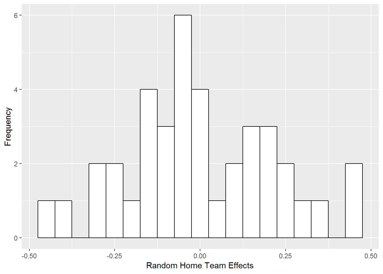
Figure 11.8: Histogram of estimated random effects for 39 home teams in Model F.

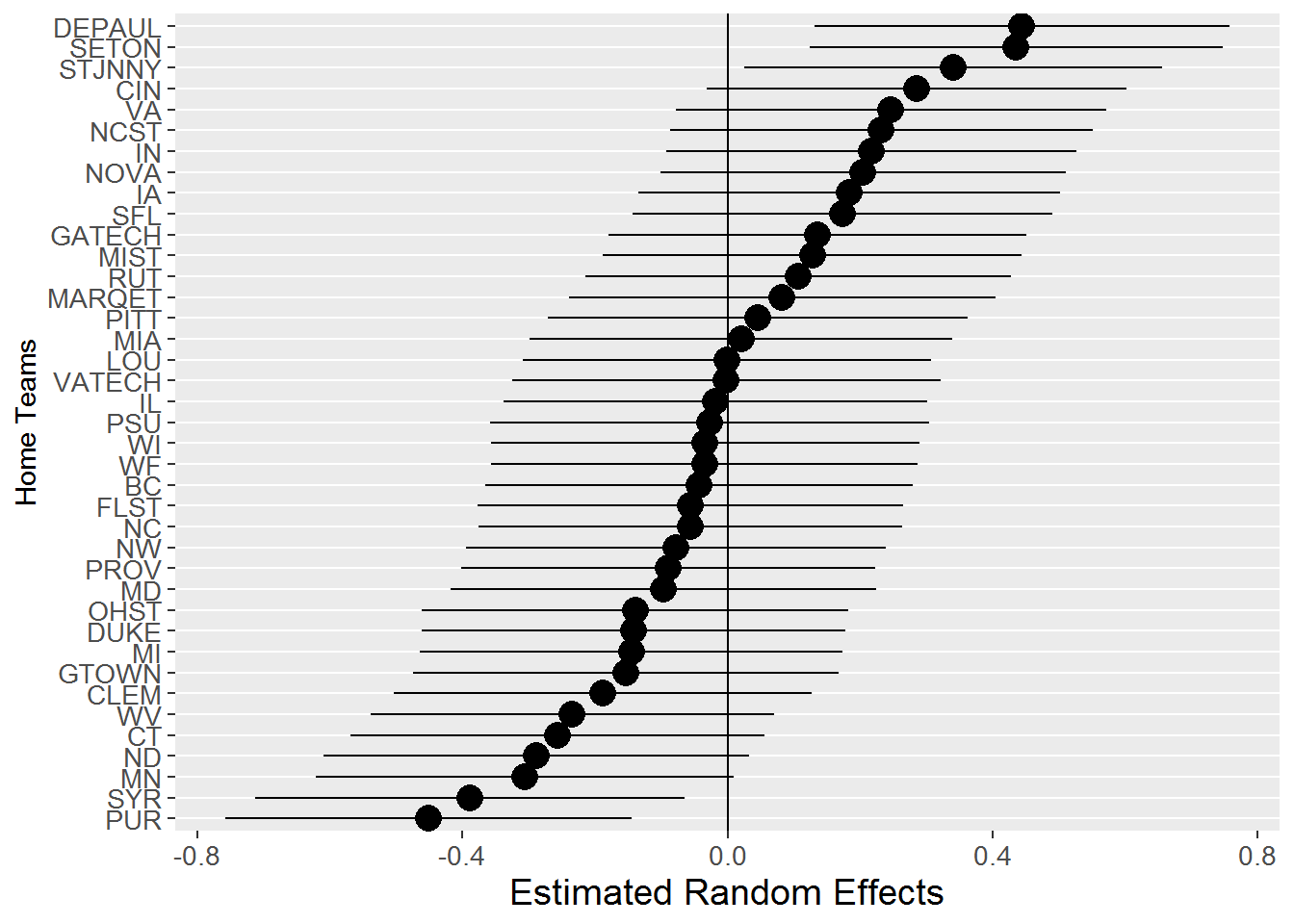
Figure 11.9: Estimated random effects and associated prediction intervals for 39 home teams in Model F.

11.9 Notes on Using R (Optional)

The R code below fits Model A.1 from Section 11.6. Note that, in glmer() or lmer(), if you have two equations at Level Two and want to fit a model with an error term for each equation, but you also want to assume that the two error terms are independent, the error terms must be requested separately. For example, “(1\(|\)hometeam)” allows the Level One intercept to vary by home team, while “(0+foul.dff\(|\)hometeam)” allows the Level One effect of foul.diff to vary by home team. Under this formulation, the correlation between those two error terms is assumed to be 0; a non-zero correlation could have been specified with “(1+foul.diff\(|\)hometeam)”.

library(lme4)

# Model A.1 (Multilevel model with only foul.diff and all 3 random effects
#             applied to both intercepts and slopes but no correlations)
model.a3 <- glmer(foul.home~ foul.diff + (1|game)+
  (1|hometeam)+(1|visitor) + (0+foul.diff|game)+(0+foul.diff|hometeam)+
  (0+foul.diff|visitor),family=binomial,data=refdata)

The R code below shows how fixef() can be used to extract the estimated fixed effects from a multilevel model. Even more, it shows how ranef() can be used to illustrate estimated random effects by Game, Home Team, and Visiting Team, along with prediction intervals for those random effects. These estimated random effects are sometimes called Empirical Bayes estimators. In this case, random effects are placed only on the “[[“(Intercept)”]]” term; the phrase “Intercept” could be replaced with other Level One covariates whose values are allowed to vary by game, home team, or visiting team in our model.

# Model F - final model?
model.f=glmer(foul.home~foul.diff+score.diff+lead.home+time+offensive+
  personal+foul.diff:offensive+foul.diff:personal+foul.diff:time+
  lead.home:time+(1|game)+(1|hometeam)+(1|visitor),family=binomial,
  data=refdata)
summary(model.f)
exp(fixef(model.f))

# Get estimated random effects based on Model F
re.int = ranef(model.f)$`game`[["(Intercept)"]]
hist(re.int,xlab="Random Effect",main="Random Effects for Game")
Home.re=ranef(model.f)$`hometeam`[["(Intercept)"]]
hist(Home.re,xlab="Random Effect",main="Random Effects for Home Team")
Visiting.re=ranef(model.f)$`visitor`[["(Intercept)"]]
hist(Visiting.re,xlab="Random Effect",
  main="Random Effects for the Visiting Team",xlim=c(-0.5,0.5))
cbind(Home.re,Visiting.re)   # 39x2 matrix of REs by team

# Prediction intervals for random effects based on Model F
ranef1=dotplot(ranef(model.f, postVar = TRUE), strip = FALSE)
print(ranef1[[3]], more = TRUE) ##HOME
print(ranef1[[2]], more = TRUE) ##VIS
print(ranef1[[1]], more = TRUE)

11.10 Exercises

11.10.1 Conceptual Exercises

Give an example of a data set and an associated research question that would best be addressed with a multilevel model for a Poisson response.
College Basketball Referees. Explain to someone unfamiliar with the plots in Figure 11.2 how to read both a conditional density plot and an empirical logit plot. For example, explain what the dark region in a conditional density plot represents, what each point in an empirical logit plot represents, etc.
With the strength of the evidence found in Figure 11.2, plots (a) and (d), is there any need to run statistical models to convince someone that referee tendencies are related to the foul differential?
In Section 11.4.2, why don’t we simply run a logistic regression model for each of the 340 games, collect the 340 intercepts and slopes, and fit a model to those intercepts and slopes?
Explain in your own words the difference between crossed and nested random effects (Section 11.5).
In the context of Case Study 9.2, describe a situation in which crossed random effects would be needed.
Assume that we added \(z_{i}\), \(r_{h}\), and \(s_{g}\) to the Level Two equation for \(b_{i}\) in Equations (11.3). (a) Give interpretations for those 3 new random effects. (b) How many additional parameters would need to be estimated (and name the new model parameters)?
In Section 11.6, could we use a likelihood ratio test to determine if it would be better to add either a random effect for home team or a random effect for visiting team to the model with a random effect for game (assuming we’re going to add one or the other)? Why or why not?
Describe how we would obtain the 1000 values representing the parametric bootstrap distribution in the histogram in Figure 11.6.
In Figure 11.6, why is it a problem that “a chi-square distribution puts too much mass in the tail” when using a likelihood ratio test to compare models?
What would be the implications of using the R expression “(foul.diff \(\mid\) game) + (foul.diff \(\mid\) hometeam) + (foul.diff \(\mid\) visitor)” in Model A.1 (Section 11.6) to obtain our variance components?
Explain the implications of having no error terms in any Level Two equations in Section 11.7 except the one for \(a_{i}\).
In the interpretation of \(\hat{\beta}_{0}\), explain why this applies to “shooting fouls at the end of the half”. Couldn’t we just say that we controlled for type of foul and time elapsed?
In the interpretation of \(\hat{\gamma}_{0}\), explain the idea that “the effect of score differential experiences a non-linear ‘bump’ at 0, where the size of the bump depends on time remaining.” Consider, for example, the effect of a point scored by the home team with 10 minutes left in the first half, depending on whether the score is tied or the home team is ahead by 2.
In the interpretation of \(\hat{\mu}_{0}\), verify the odds increases of 29.6% for shooting fouls and 43.6% for offensive fouls. Where does the stated 10.9% increase factor in?
We could also interpret the interaction between two quantitative variables described by \(\hat{\omega}_{0}\) as “the effect of time remaining increases by 0.9% for each extra foul on the visiting team, after controlling for …” Numerically illustrate this interpretation by considering foul differentials of 2 (the home team has 2 more fouls than the visitors) and -2 (the visitors have 2 more fouls than the home team).
Provide interpretations in context for \(\hat{\phi}_{0}\), \(\hat{\kappa}_{0}\), and \(\hat{\xi}_{0}\).
In Section 11.8, why isn’t the baseline odds of a home foul for DePaul considered a model parameter?
Heart attacks in Aboriginal Australians. Randall, et al., published a 2014 article in Health and Place entitled “Exploring disparities in acute myocardial infarction events between Aboriginal and non-Aboriginal Australians: Roles of age, gender, geography and area-level disadvantage.” They used multilevel Poisson models to compare rates of acute myocardial infarction (AMI) in the 199 Statistical Local Areas (SLAs) in New South Wales. Within SLA, AMI rates (number of events over population count) were summarized by subgroups determined by year (2002-2007), age (in 10-year groupings), sex, and Aboriginal status; these are then our Level One variables. Analyses also incorporated remoteness (classified by quartiles) and socio-economic status (classified by quintiles) assessed at the SLA level (Level Two) (Randall et al. 2014). For this study, give the observational units at Levels One and Two.
Table 11.4 shows Table 2 from Randall et al. (2014). Let \(Y_{ij}\) be the number of acute myocardial infarctions in subgroup \(j\) from SLA \(i\); write out the multilevel model that likely produced Table 11.4. How many fixed effects and variance components must be estimated?

Table 11.4: Adjusted rate ratios for individual-level variables from the multilevel Poisson regression model with random intercept for area from Table 2 in Randall et al. (2014).

	RR	95% CI	p-Value
Aboriginal
No(ref)	1		<0.01
Yes	2.1	1.98-2.23
Age Group
25-34 (ref)	1		<0.01
35-44	6.01	5.44-6.64
45-54	19.36	17.58-21.31
55-64	40.29	36.67-44.26
65-74	79.92	72.74-87.80
75-84	178.75	162.70-196.39
Sex
Male (ref)	1		<0.01
Female	0.45	0.44-0.45
Year
2002 (ref)	1		<0.01
2003	1	0.98-1.03
2004	0.97	0.95-0.99
2005	0.91	0.89-0.94
2006	0.88	0.86-0.91
2007	0.88	0.86-0.91

Provide interpretations in context for the bolded rate ratios, confidence intervals, and p-values in Table 11.4.
Given the rate ratio and 95% confidence interval reported for Aboriginal Australians in Table 11.4, find the estimated model fixed effect for Aboriginal Australians from the multilevel model along with its standard error.
How might the p-value for Age have been produced?
Randall et al. (2014) report that “we identified a significant interaction between Aboriginal status and age group (\(p<0.01\)) and Aboriginal status and sex (\(p<0.01\)), but there was no significant interaction between Aboriginal status and year (p=0.94).” How would the multilevel model associated with Table 11.4 need to have been adjusted to allow these interactions to be tested?
Table 11.5 shows Table 3 from Randall et al. (2014). Describe the changes to the multilevel model for Table 11.4 that likely produced this new table.
Provide interpretations in context for the bolded rate ratios, confidence intervals, and p-values in Table 11.5.

Table 11.5: Adjusted rate ratios for area-level variables from the multilevel Poisson regression model with random intercept for area from Table 3 in Randall et al. (2014).

	RR	95% CI	p-Value
Remoteness of Residence*
Major City	1		<0.01
Inner Regional	1.16	1.04-1.28
Outer Regional	1.11	1.01-1.23
Remote/very remote	1.22	1.02-1.45
SES quintile*
1 least disadvantaged	1		<0.01
2	1.26	1.11-1.43
3	1.4	1.24-1.58
4	1.46	1.30-1.64
5 most disadvantaged	1.7	1.52-1.91

Area-level factors added one at a time to the fully adjusted individual-level model (adjusted for Aboriginal status, age, sex and year) due to being highly associated.

Randall et al. (2014) also report the results of a single-level Poisson regression model: “After adjusting for age, sex and year of event, the rate of AMI events in Aboriginal people was 2.3 times higher than in non-Aboriginal people (95% CI: 2.17-2.44).” Compare this to the results of the multilevel Poisson model; what might explain any observed differences?
Randall et al. (2014) claim that “our application of multilevel modelling techniques allowed us to account for clustering by area of residence and produce ‘shrunken’ small-area estimates, which are not as prone to random fluctuations as crude or standardised rates.” Explain what they mean by this statement.

11.10.2 Open-ended Exercises

Airbnb in Chicago. Trinh and Ameri (2018) collected data on 1561 Airbnb listings in Chicago from August 2016, and then they merged in information from the neighborhood (out of 43 in Chicago) where the listing was located. We can examine traits that are associated with listings that achieve an overall satisfaction of 5 out of 5 vs. those that do not (i.e. treat satisfaction as a binary variable). Conduct an EDA, build a generalized multilevel model, and interpret model coefficients to answer questions such as: What are characteristics of a higher rated listing? Are the most influential traits associated with individual listings or entire neighborhoods? Are there intriguing interactions where the effect of one variable depends on levels of another?

The following variables can be found in airbnb.csv or derived from the variables found there:

overall_satisfaction = rating on a 0-5 scale.
satisfaction = 1 if overall_satisfaction is 5, 0 otherwise
price = price for one night (in dollars)
reviews = number of reviews posted
room_type = Entire home/apt, Private room, or Shared room
accommodates = number of people the unit can hold
bedrooms = number of bedrooms
minstay = minimum length of stay (in days)
neighborhood = neighborhood where unit is located (1 of 43)
district = district where unit is located (1 of 9)
WalkScore = quality of the neighborhood for walking (0-100)
TransitScore = quality of the neighborhood for public transit (0-100)
BikeScore = quality of the neighborhood for biking (0-100)
PctBlack = proportion of black residents in a neighborhood
HighBlack = 1 if PctBlack above .60, 0 otherwise

Seed Germination. We will return to the data from Angell (2010) used in Case Study 10.2, but whether or not a seed germinated will be considered the response variable rather than the heights of germinated plants. We will use the wide data set (one row per plant) seeds2.csv for this analysis as described in Section 10.3.1, although we will ignore plant heights over time and focus solely on if the plant germinated at any time. Use generalized linear multilevel models to determine the effects of soil type and sterilization on germination rates; perform separate analyses for coneflowers and leadplants, and describe differences between the two species. Support your conclusions with well-interpreted model coefficients and insightful graphical summaries.
Book Banning. The risk of literature censorship is constant, with provocative literature risking being challenged and subsequently being banned. Reasons for censorship have changed over time, with modern day challenges more likely to be for reasons relating to obscenity and child protection rather than overt political and religious objections (Jenkins 2008). Many past studies have addressed chiefly the reasons listed by those who challenge a book, but few examine the overall context in which books are banned—for example, the characteristics of the states in which they occur.

A team of students assembled a data set by starting with information on book challenges from the American Library Society (Fast and Hegland 2011). These book challenges—an initiation of the formal procedure for book censorship—occurred in US States between January of 2000 and November of 2010. In addition, state-level demographic information was obtained from the US Census Bureau and the Political Value Index (PVI) was obtained from the Cook Political Report.

We will consider a data set with 931 challenges and 18 variables. All book challenges over the nearly 11 year period are included except those from the State of Texas; Texas featured 683 challenges over this timeframe, nearly 5 times the number in the next largest state. Thus, the challenges from Texas have been removed and could be analyzed separately. Here, then, is a description of available variables in bookbanningNoTex.csv:
- book = unique book ID number
- booktitle = name of book
- author = name of author
- state = state where challenge made
- removed = 1 if book was removed (challenge was successful); 0 otherwise
- pvi2 = state score on the Political Value Index, where positive indicates a Democratic leaning, negative indicates a Republican leaning, and 0 is neutral
- cperhs = percentage of high school graduates in a state (grand mean centered)
- cmedin = median state income (grand median centered)
- cperba = percentage of college graduates in a state (grand mean centered)
- days2000 = date challenge was made, measured by number of days after January 1, 2000
- obama = 1 if challenge was made while Barack Obama was President; 0 otherwise
- freqchal = 1 if book was written by a frequently challenged author (10 or more challenges across the country); 0 otherwise
- sexexp = 1 if reason for challenge was sexually explicit material; 0 otherwise
- antifamily = 1 if reason for challenge was antifamily material; 0 otherwise
- occult = 1 if reason for challenge was material about the occult; 0 otherwise
- language = 1 if reason for challenge was inappropriate language; 0 otherwise
- homosexuality = 1 if reason for challenge was material about homosexuality; 0 otherwise
- violence = 1 if reason for challenge was violent material; 0 otherwise
The primary response variable is removed. Certain potential predictors are measured at the state level (e.g., pvi2 and cperhs), at least one is at the book level (freqchal), and several are specific to an individual challenge (e.g., obama and sexexp). In addition, note that the same book can be challenged for more than one reason, in different states, or even at different times in the same state.

Perform exploratory analyses and then run multilevel models to examine significant determinants of successful challenges. Write a short report comparing specific reasons for the challenge to the greater context in which a challenge was made.

References

Anderson, Kyle J., and David A. Pierce. 2009. “Officiating Bias: The Effect of Foul Differential on Foul Calls in Ncaa Basketball.” Journal of Sports Sciences 27 (7): 687–94. doi:10.1080/02640410902729733.

Moskowitz, Tobias J., and L. Jon Wertheim. 2011. Scorecasting: The Hidden Influences Behind How Sports Are Played and Games Are Won. New York: Crown Archetype.

Noecker, Cecilia A., and Paul Roback. 2012. “New Insights on the Tendency of Ncaa Basketball Officials to Even Out Foul Calls.” Journal of Quantitative Analysis in Sports 8 (3): 1–23.

Randall, D.A., L.R. Jorm, S. Lujic, S.J. Eades, T.R. Churches, A.J. O’Loughlin, and A.H. Leyland. 2014. “Exploring Disparities in Acute Myocardial Infarction Events Between Aboriginal and Non-Aboriginal Australians: Roles of Age, Gender, Geography and Area-Level Disadvantage.” Health & Place 28: 58–66. doi:https://doi.org/10.1016/j.healthplace.2014.03.009.

Trinh, Ly, and Pony Ameri. 2018. “Airbnb Price Determinants: A Multilevel Modeling Approach.” Project for Statistics 316-Advanced Statistical Modeling, St. Olaf College.

Angell, Diane. 2010. “Effects of Soil Type and Sterilization on the Growth of Coneflowers and Leadplants.” Class data for Biology 261-Ecological Principles, St. Olaf College.

Jenkins, Christine A. 2008. “Book Challenges, Challenging Books, and Young Readers: The Research Picture.” Language Arts 85 (3): 228–36.

Fast, Shannon, and Thomas Hegland. 2011. “Book Challenges: A Statistical Examination.” Project for Statistics 316-Advanced Statistical Modeling, St. Olaf College.