5.3 Generating random data

Because R is a language built for statistics, it contains many functions that allow you generate random data – either from a vector of data that you specify (like Heads or Tails from a coin), or from an established probability distribution, like the Normal or Uniform distribution.

In the next section we’ll go over the standard sample() function for drawing random values from a vector. We’ll then cover some of the most commonly used probability distributions: Normal and Uniform.

5.3.1 sample()

Argument	Definition
x	A vector of outcomes you want to sample from. For example, to simulate coin flips, you’d enter x = c("H", "T")
size	The number of samples you want to draw. The default is the length of x.
replace	Should sampling be done with replacement? If FALSE (the default value), then each outcome in x can only be drawn once. If TRUE, then each outcome in x can be drawn multiple times.
prob	A vector of probabilities of the same length as x indicating how likely each outcome in x is. The vector of probabilities you give as an argument should add up to one. If you don’t specify the prob argument, all outcomes will be equally likely.

The sample() function allows you to draw random samples of elements (scalars) from a vector. For example, if you want to simulate the 100 flips of a fair coin, you can tell the sample function to sample 100 values from the vector [“Heads”, “Tails”]. Or, if you need to randomly assign people to either a “Control” or “Test” condition in an experiment, you can randomly sample values from the vector [“Control”, “Test”]:

Let’s use sample() to draw 10 samples from a vector of integers from 1 to 10.

# From the integers 1:10, draw 5 numbers
sample(x = 1:10, size  = 5)
## [1] 8 7 5 9 2

5.3.1.1 replace = TRUE

If you don’t specify the replace argument, R will assume that you are sampling without replacement. In other words, each element can only be sampled once. If you want to sample with replacement, use the replace = TRUE argument:

Think about replacement like drawing balls from a bag. Sampling with replacement (replace = TRUE) means that each time you draw a ball, you return the ball back into the bag before drawing another ball. Sampling without replacement (replace = FALSE) means that after you draw a ball, you remove that ball from the bag so you can never draw it again.

# Draw 30 samples from the integers 1:5 with replacement
sample(x = 1:5, size = 10, replace = TRUE)
##  [1] 1 1 4 4 1 3 3 4 3 1

If you try to draw a large sample from a vector replacement, R will return an error because it runs out of things to draw:

# You CAN'T draw 10 samples without replacement from
#  a vector with length 5
sample(x = 1:5, size = 10)

Error: cannot take a sample larger than the population when ‘replace = FALSE’

To fix this, just tell R that you want to sample with replacement:

# You CAN draw 10 samples with replacement from a
#  vector of length 5
sample(x = 1:5, size = 10, replace = TRUE)
##  [1] 4 2 4 1 4 5 5 2 4 3

To specify how likely each element in the vector x should be selected, use the prob argument. The length of the prob argument should be as long as the x argument. For example, let’s draw 10 samples (with replacement) from the vector [“a”, “b”], but we’ll make the probability of selecting “a” to be .90, and the probability of selecting “b” to be .10

sample(x = c("a", "b"), 
       prob = c(.9, .1),
       size = 10, 
       replace = TRUE)
##  [1] "a" "a" "a" "a" "a" "a" "a" "a" "a" "a"

5.3.1.2 Ex: Simulating coin flips

Let’s simulate 10 flips of a fair coin, were the probably of getting either a Head or Tail is .50. Because all values are equally likely, we don’t need to specify the prob argument

sample(x = c("H", "T"), # The possible values of the coin
       size = 10,  # 10 flips
       replace = TRUE) # Sampling with replacement
##  [1] "H" "H" "T" "H" "T" "H" "H" "H" "T" "T"

Now let’s change it by simulating flips of a biased coin, where the probability of Heads is 0.8, and the probability of Tails is 0.2. Because the probabilities of each outcome are no longer equal, we’ll need to specify them with the prob argument:

sample(x = c("H", "T"),
       prob = c(.8, .2), # Make the coin biased for Heads
       size = 10,
       replace = TRUE)
##  [1] "T" "H" "H" "H" "H" "H" "H" "H" "T" "H"

As you can see, our function returned a vector of 10 values corresponding to our sample size of 10.

5.3.1.3 Ex: Coins from a chest

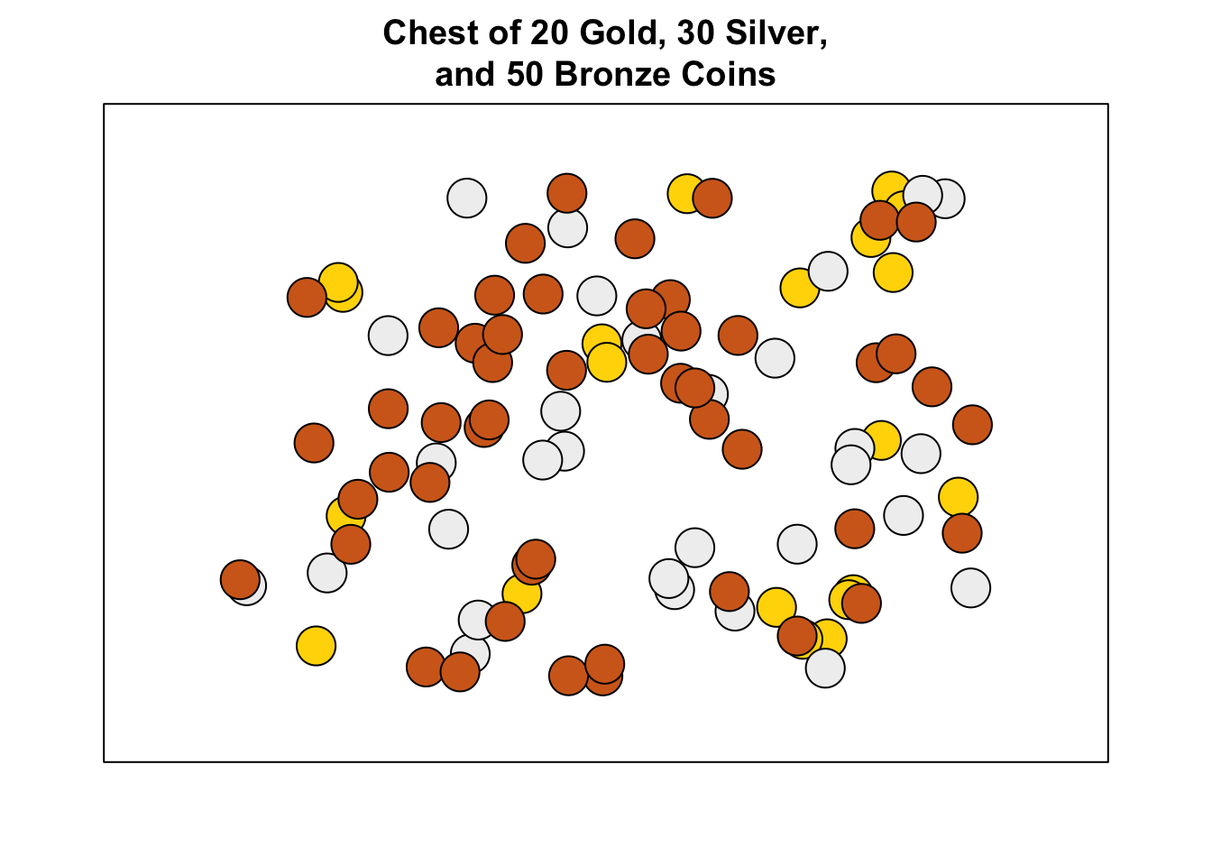
Now, let’s sample drawing coins from a treasure chest Let’s say the chest has 100 coins: 20 gold, 30 silver, and 50 bronze. Let’s draw 10 random coins from this chest.

# Create chest with the 100 coins

chest <- c(rep("gold", 20),
         rep("silver", 30),
         rep("bronze", 50))

# Draw 10 coins from the chest
sample(x = chest,
       size = 10)
##  [1] "silver" "bronze" "silver" "bronze" "gold"   "bronze" "bronze"
##  [8] "bronze" "bronze" "gold"

The output of the sample() function above is a vector of 10 strings indicating the type of coin we drew on each sample. And like any random sampling function, this code will likely give you different results every time you run it! See how long it takes you to get 10 gold coins…

In the next section, we’ll cover how to generate random data from specified probability distributions. What is a probability distribution? Well, it’s simply an equation – also called a likelihood function – that indicates how likely certain numerical values are to be drawn.

We can use probability distributions to represent different types of data. For example, imagine you need to hire a new group of pirates for your crew. You have the option of hiring people from one of two different pirate training colleges that produce pirates of varying quality. One college “Pirate Training Unlimited” might tend to pirates that are generally ok - never great but never terrible. While another college “Unlimited Pirate Training” might produce pirates with a wide variety of quality, from very low to very high. In Figure 5.4 I plotted 5 example pirates from each college, where each pirate is shown as a ball with a number written on it. As you can see, pirates from PTU all tend to be clustered between 40 and 60 (not terrible but not great), while pirates from UPT are all over the map, from 0 to 100. We can use probability distributions (in this case, the uniform distribution) to mathematically define how likely any possible value is to be drawn at random from a distribution. We could describe Pirate Training Unlimited with a uniform distribution with a small range, and Unlimited Pirate Training with a second uniform distribution with a wide range.

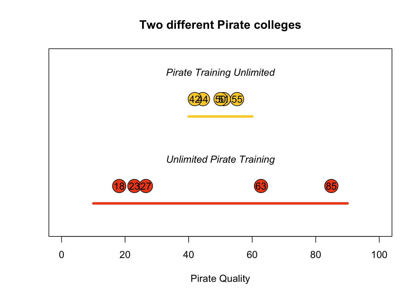
Figure 5.4: Sampling 5 potential pirates from two different pirate colleges. Pirate Training Unlimited (PTU) consistently produces average pirates (with scores between 40 and 60), while Unlimited Pirate Training (UPT), produces a wide range of pirates from 0 to 100.

In the next two sections, I’ll cover the two most common distributions: The Normal and the Uniform. However, R contains many more distributions than just these two. To see them all, look at the help menu for Distributions:

# See all distributions included in Base R
?Distributions

5.3.2 Normal (Gaussian)

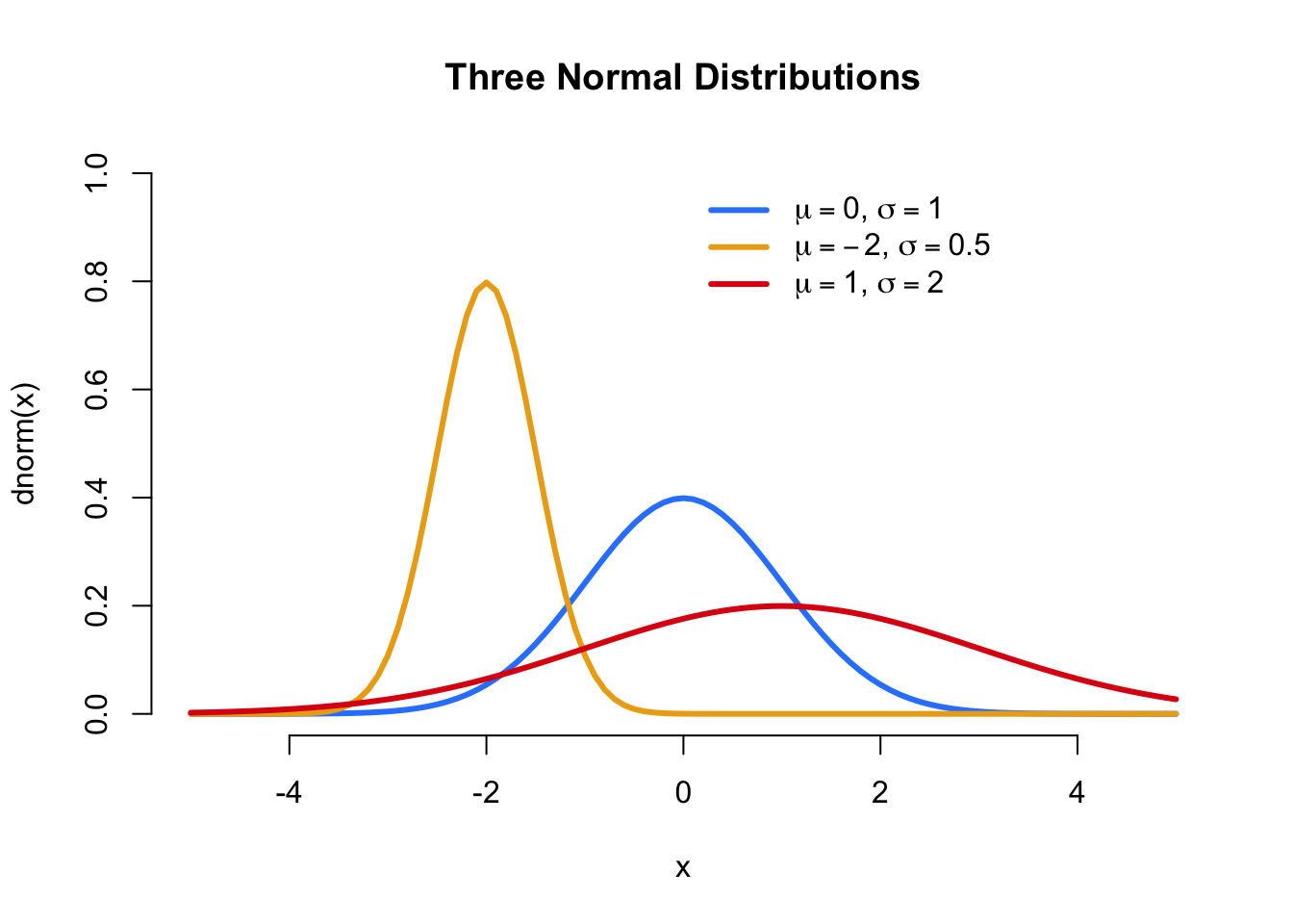
Figure 5.5: Three different normal distributions with different means and standard deviations

Argument	Definition
n	The number of observations to draw from the distribution.
mean	The mean of the distribution.
sd	The standard deviation of the distribution.

The Normal (a.k.a “Gaussian”) distribution is probably the most important distribution in all of statistics. The Normal distribution is bell-shaped, and has two parameters: a mean and a standard deviation. To generate samples from a normal distribution in R, we use the function rnorm()

# 5 samples from a Normal dist with mean = 0, sd = 1
rnorm(n = 5, mean = 0, sd = 1)
## [1] -0.0046 -0.0016  1.2226  1.2509  1.8195

# 3 samples from a Normal dist with mean = -10, sd = 15
rnorm(n = 3, mean = -10, sd = 15)
## [1] -10.67   0.61 -25.94

Again, because the sampling is done randomly, you’ll get different values each time you run rnorm()

5.3.3 Uniform

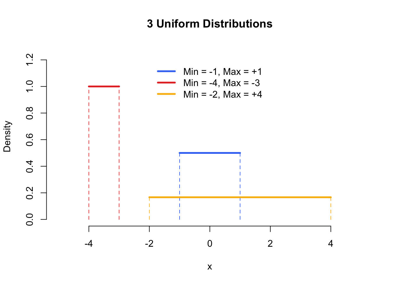
Figure 5.6: The Uniform distribution - known colloquially as the Anthony Davis distribution.

Next, let’s move on to the Uniform distribution. The Uniform distribution gives equal probability to all values between its minimum and maximum values. In other words, everything between its lower and upper bounds are equally likely to occur. To generate samples from a uniform distribution, use the function runif(), the function has 3 arguments:

Argument	Definition
n	The number of observations to draw from the distribution.
min	The lower bound of the Uniform distribution from which samples are drawn
max	The upper bound of the Uniform distribution from which samples are drawn

Here are some samples from two different Uniform distributions:

# 5 samples from Uniform dist with bounds at 0 and 1
runif(n = 5, min = 0, max = 1)
## [1] 0.0019 0.8019 0.1661 0.3628 0.9268

# 10 samples from Uniform dist with bounds at -100 and +100
runif(n = 10, min = -100, max = 100)
##  [1] -10.8 -37.7   2.2 -38.4 -34.6  46.2 -68.8   5.3  92.9 -14.4

5.3.4 Notes on random samples

5.3.4.1 Random samples will always change

Every time you draw a sample from a probability distribution, you’ll (likely) get a different result. For example, see what happens when I run the following two commands (you’ll learn the rnorm() function on the next page…)

# Draw a sample of size 5 from a normal distribution with mean 100 and sd 10
rnorm(n = 5, mean = 100, sd = 10)
## [1] 102  94 100  85  98

# Do it again!
rnorm(n = 5, mean = 100, sd = 10)
## [1] 119  99  96  97 115

As you can see, the exact same code produced different results – and that’s exactly what we want! Each time you run rnorm(), or another distribution function, you’ll get a new random sample.

5.3.4.2 Use set.seed() to control random samples

There will be cases where you will want to exert some control over the random samples that R produces from sampling functions. For example, you may want to create a reproducible example of some code that anyone else can replicate exactly. To do this, use the set.seed() function. Using set.seed() will force R to produce consistent random samples at any time on any computer.

In the code below I’ll set the sampling seed to 100 with set.seed(100). I’ll then run rnorm() twice. The results will always be consistent (because we fixed the sampling seed).

# Fix sampling seed to 100, so the next sampling functions
#   always produce the same values
set.seed(100)

# The result will always be -0.5022, 0.1315, -0.0789
rnorm(3, mean = 0, sd = 1)
## [1] -0.502  0.132 -0.079

# The result will always be 0.887, 0.117, 0.319
rnorm(3, mean = 0, sd = 1)
## [1] 0.89 0.12 0.32

Try running the same code on your machine and you’ll see the exact same samples that I got above. Oh and the value of 100 I used above in set.seed(100) is totally arbitrary – you can set the seed to any integer you want. I just happen to like how set.seed(100) looks in my code.