2.4 Poisson
Poisson distributions are used to model the number of events occurring in a fixed period of time. In Poisson processes, events occur continuously and independently at a constant average rate. This blog by Aerin Kim demonstrates how the Poisson distribution is related to the binomial distribution. The key is that the binomial distribution expresses the probability of \(X = k\) events in \(n\) trials when the probability of one event in one trial is \(p\). Sometimes you don’t know \(p\), but instead know that \(\lambda\) events occur per some time interval. You could try to back into the binomial by shrinking the time interval so that \(k\) could never be greater than one. The ratio \(p = \lambda / n\) approaches the probability of observing one event in one trial as \(n \rightarrow \infty\). As \(n \rightarrow \infty\), \(p \rightarrow 0\). If you do this and follow the math, you wind up with the Poisson distribution!
\[\begin{eqnarray} P(X = k) &=& \mathrm{lim}_{n \rightarrow \infty} {n \choose k}p^k(1-p)^{n-k}\\ &=& \mathrm{lim}_{n \rightarrow \infty} \frac{n!}{(n-k)!k!} \left(\frac{\lambda}{n}\right)^k \left(1-\frac{\lambda}{n}\right)^{n-k}\\ &=& \mathrm{lim}_{n \rightarrow \infty} \frac{n!}{(n-k)!k!} \left(\frac{\lambda}{n}\right)^k \left(1-\frac{\lambda}{n}\right)^n\left(1-\frac{\lambda}{n}\right)^{-k}\\ &=& \mathrm{lim}_{n \rightarrow \infty} \frac{n!}{(n-k)!k!} \left(\frac{\lambda}{n}\right)^k \left(e^{-\lambda}\right)(1)\\ &=& \mathrm{lim}_{n \rightarrow \infty} \frac{n!}{(n-k)!n^k} e^{-\lambda}\frac{\lambda^k}{k!} \\ &=& e^{-\lambda}\frac{\lambda^k}{k!} \end{eqnarray}\]
I didn’t get that last step, but I’ll take it on faith.
If \(X\) is the number of successes in \(n\) (many) trials when the probability of success \(\lambda / n\) is small, then \(X\) is a random variable with a Poisson distribution \(X \sim \mathrm{Pois}(\lambda)\)
\[f(X = k;\lambda) = \frac{e^{-\lambda} \lambda^k}{k!} \hspace{1cm} k \in (0, 1, ...), \hspace{2mm} \lambda > 0\]
with \(E(X)=\lambda\) and \(\mathrm{Var}(X) = \lambda\).
The Poisson distribution is also related to the exponential distribution. If the number of events per unit time follows a Poisson distribution, then the amount of time between events follows the exponential distribution.
The Poisson likelihood function is
\[L(\lambda; k) = \prod_{i=1}^N f(k_i; \lambda) = \prod_{i=1}^N \frac{e^{-\lambda} \lambda^k_i}{k_i !} = \frac{e^{-n \lambda} \lambda^{\sum k_i}}{\prod k_i}.\]
The Poisson loglikelihood function is
\[l(\lambda; k) = \sum_{i=1}^N k_i \log \lambda - n \lambda.\]
The loglikelihood function is maximized at
\[\hat{\lambda} = \sum_{i=1}^N k_i / n.\]
Thus, for a Poisson sample, the MLE for \(\lambda\) is just the sample mean.
Consider data set dat_pois containing frequencies counts of goals scored per match during a soccer tournament. Totals ranged from 0 to 8.
##   goals freq
## 1     0   23
## 2     1   37
## 3     2   20
## 4     3   11
## 5     4    2
## 6     5    1
## 7     6    0
## 8     7    0
## 9     8    1
The MLE of \(\lambda\) is the sample weighted mean.
(lambda <- weighted.mean(dat_pois$goals, dat_pois$freq))
## [1] 1.378947
The 0.95 CI is \(\lambda \pm z_{.05/2} \sqrt{\lambda / n}\)
n <- sum(dat_pois$freq)
z <- qnorm(0.975)
se <- sqrt(lambda / n)
lambda + c(-z*se, +z*se)
## [1] 1.142812 1.615082
The expected probability of scoring 2 goals in a match is \(\frac{e^{-1.38} 1.38^2}{2!} = 0.239\).
dpois(x = 2, lambda = lambda)
## [1] 0.2394397
The expected probability of scoring 2 to 4 goals in a match is
ppois(q = 4, lambda = lambda) -
  ppois(q = 1, lambda = lambda)
## [1] 0.3874391data.frame(events = 0:10,
pmf = dpois(0:10, lambda),
cdf = ppois(0:10, lambda, lower.tail = TRUE)) %>%
ggplot() +
geom_col(aes(x = factor(events), y = pmf)) +
geom_text(aes(x = factor(events), label = round(pmf, 3), y = pmf + 0.01),
position = position_dodge(0.9), size = 3, vjust = 0) +
geom_line(aes(x = events, y = cdf/2), size = 1) +
scale_y_continuous(limits = c(0, .5),
sec.axis = sec_axis(~ . * 2, name = "Cum Prob")) +
labs(title = "PMF and CDF of Poisson Distribution",
subtitle = paste0("Pois(", scales::comma(lambda, accuracy = .01), ")"),
x = "X = k", y = "Density")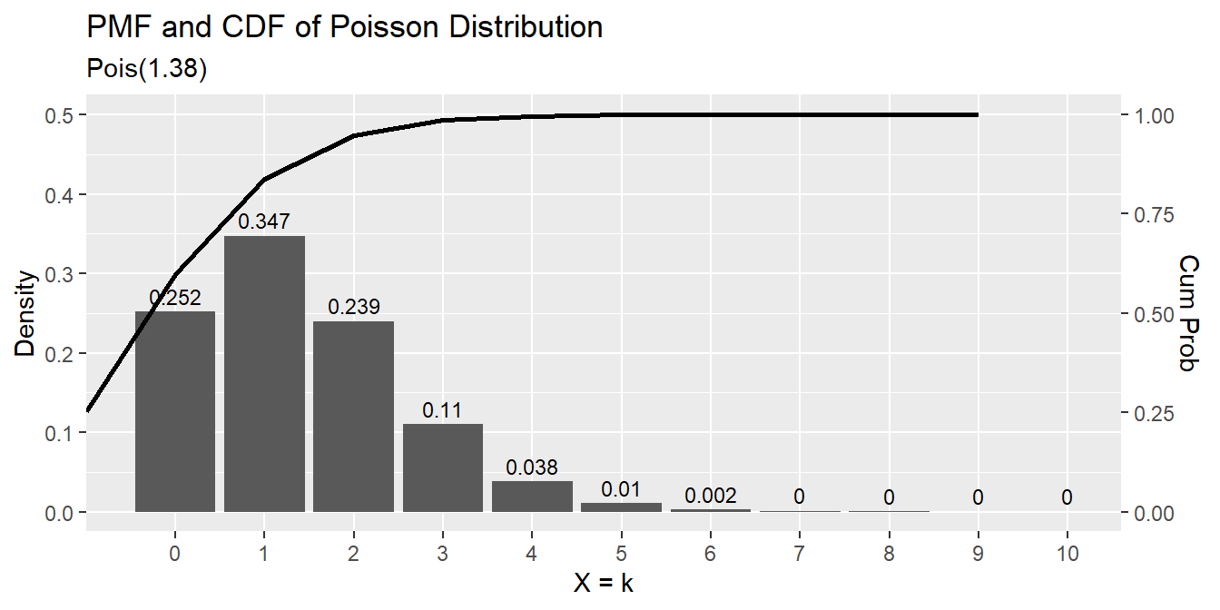
How well does the Poisson distribution fit the dat_pois data set?
dat_pois %>%
  mutate(pred = n * dpois(x = goals, lambda = lambda)) %>%
  rename(obs = freq) %>%
  pivot_longer(cols = -goals) %>%
  ggplot(aes(x = goals, y = value, color = name)) +
  geom_point() +
#  geom_smooth(se = FALSE) +
  theme(legend.position = "top") +
  labs(
    title = "Poisson Dist: Observed vs Expected",
    color = "",
    y = "frequencey"
  )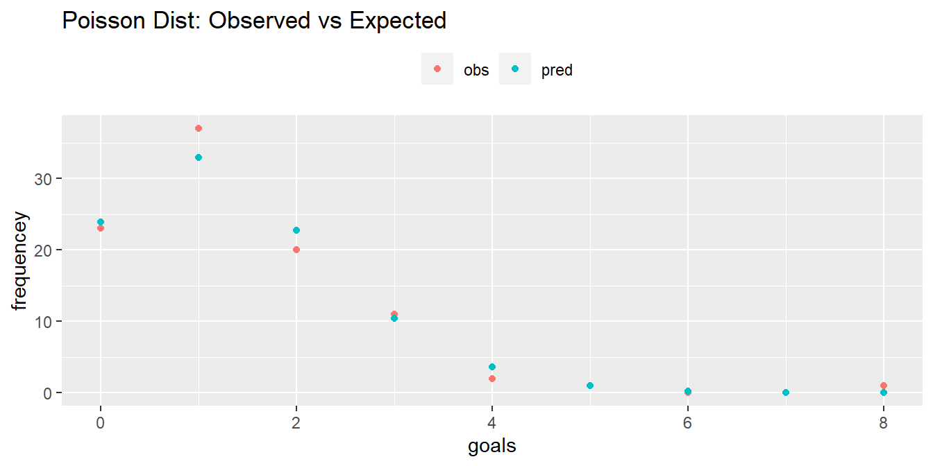
It seems to fit pretty good! Run a chi-square goodness-of-fit test to confirm. The test requires an expected frequency of at least 5 per cell. Cells 4 through 8 are under 5, so you need to lump them.
x <- dat_pois %>%
  group_by(goals = if_else(goals >= 4, 4, goals)) %>%
  summarize(.groups = "drop", freq = sum(freq)) %>%
  pull(freq)
p <- dat_pois %>%
  mutate(p = dpois(x = goals, lambda = lambda)) %>%
  group_by(goals = if_else(goals >= 4, 4, goals)) %>%
  summarize(.groups = "drop", p = sum(p)) %>%
  pull(p)
(chisq_test <- chisq.test(x = x, p = p, rescale.p = TRUE))
##
## Chi-squared test for given probabilities
##
## data: x
## X-squared = 1.0414, df = 4, p-value = 0.9035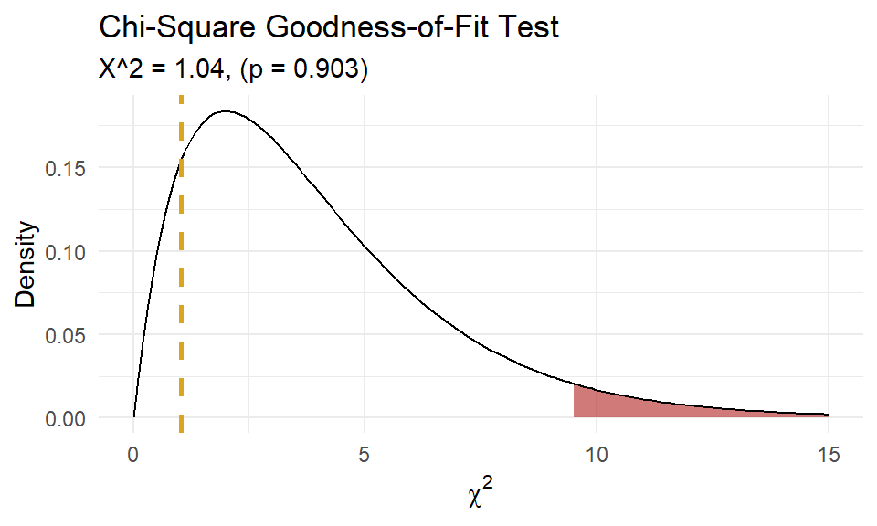
A chi-square goodness-of-fit test was conducted to determine whether the matches had the same proportion of goals as the theoretical Poisson distribution. The minimum expected frequency was 5. The chi-square goodness-of-fit test indicated that the number of matches with 0, 1, 2, 3, or 4 or more goals was not statistically significantly different from the proportions expected in the theoretical Poisson distribution (\(\chi^2\)(4) = 1.041, p = 0.903).
As demonstrated at the beginning of this section, the \(\mathrm{Pois}(\lambda)\) approaches the \(\mathrm{Bin}(n, \pi)\) where \(\lambda = n\pi\) when \(n \rightarrow \infty\) and \(\pi \rightarrow 0\). The Poisson is a useful (computationally inexpensive) approximation to the binomial when \(n \ge 20)\) and \(\pi \le 0.05\). For example, suppose a baseball player has a \(\pi = .03\) chance of hitting a home run. What is the probability of hitting \(X \ge 20\) home runs in \(n = 500\) at-bats? This is a binomial process because the sample size is fixed.
pbinom(q = 20, size = 500, prob = 0.03, lower.tail = FALSE)## [1] 0.07979678But \(n\) is large and \(\pi\) is small, so the Poisson distribution works well too.
ppois(q = 20, lambda = 0.03 * 500, lower.tail = FALSE)## [1] 0.08297091n = 500
p = 0.03
x = 0:30
data.frame(
events = x,
Poisson = dpois(x = x, lambda = p * n),
Binomial = dbinom(x = x, size = n, p = p)
) %>%
pivot_longer(cols = -events) %>%
ggplot(aes(x = events, y = value, color = name)) +
geom_line() +
theme(legend.position = "top") +
labs(title = "Pois(.03*500) vs. Bin(500, .03)",
subtitle = "Poisson approximation to binomial.",
x = "Events",
y = "Density",
color = "")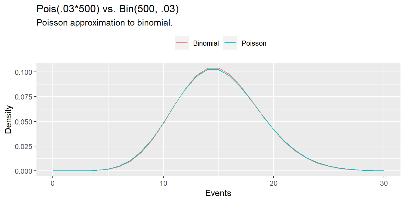
When the observed variance is greater than \(\lambda\) (overdispersion), the Negative Binomial distribution can be used instead of Poisson.