2.5 Exponential

Exponential distributions are usually used to model the elapsed time between events in a Poisson process.

If \(X\) is the time to the next successful event in a Poisson process where the average rate of events is \(\lambda\), then \(X\) is a random variable with an exponential distribution \(X \sim \mathrm{Exp}(\lambda)\)

\[ f(X = x; \lambda) = \begin{cases} \lambda e^{-\lambda x}, & \mbox{if } x \ge 0 \\ 0, & \mbox{if } x < 0 \end{cases} \]

with \(E(X)=1/\lambda\) and \(Var(X) = 1/\lambda^2\).

This blog by Aerin Kim demonstrates how the exponential distribution is related to the Poisson distribution. The key is that the probability of no event in 1 time period is \(P(X = 0; \lambda) = e^{-\lambda}\frac{\lambda^0}{0!} = e^{-\lambda}\), so the probability of no events in t time periods is \(P(X>t) =e^{-\lambda t}\) because the \(t\) periods are independent. The CDF is \(P(X \le t) =1 - e^{-\lambda t}\). And the PDF is its derivative, \(P(X = t) = \lambda e^{-\lambda t}\)

Kim shows how the exponential distribution is “memory-less,” meaning the \(P(X > x_1 | X > x_0) = P(X > x_1 - x_0).\) E.g., the probability a 9-year old machine fails after 12 years is the same as the probability a 0-year old machine fails after 3 years. If that seems like a bad model, turn to something with increasing hazard rates, like Weibull. But oftentimes it is a good assumption, like the probability of a car accident (this is the context in which you might refer to \(\lambda\) as the hazard rate).

Suppose the average rate of bus arrivals is one per 15 minutes, a Poisson process. The probability less than 10 minutes elapses between buses is \(P(X \le 10) = 1 - e^{-1/15 \cdot 10} = .486.\)

data.frame(min = 0:60) %>% mutate(p = pexp(min, 1/15)) %>%
  ggplot(aes(x = min)) +
  geom_line(aes(y = p)) +
  geom_hline(yintercept = pexp(10, 1/15), linetype = 2) +
  geom_vline(xintercept = 10, linetype = 2) +
  scale_y_continuous(breaks = seq(0, 1, .1)) +
  scale_x_continuous(breaks = seq(0, 60, 5)) +
  theme(panel.grid.minor = element_blank()) +
  labs(title = "P(X<=10) = .486")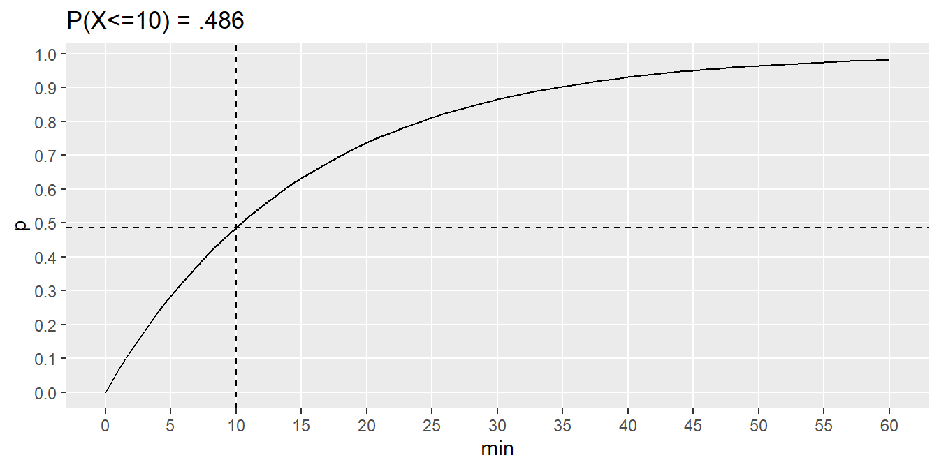

90% of buses arrive within 34.5 minutes.

data.frame(min = 0:60) %>% mutate(p = pexp(min, 1/15)) %>%
  ggplot(aes(x = min)) +
  geom_line(aes(y = p)) +
  geom_hline(yintercept = 0.90, linetype = 2) +
  geom_vline(xintercept = qexp(.90, 1/15), linetype = 2) +
  scale_y_continuous(breaks = seq(0, 1, .1)) +
  scale_x_continuous(breaks = seq(0, 60, 5)) +
  theme(panel.grid.minor = element_blank()) +
  labs(title = "P(X<=34.5) = .90")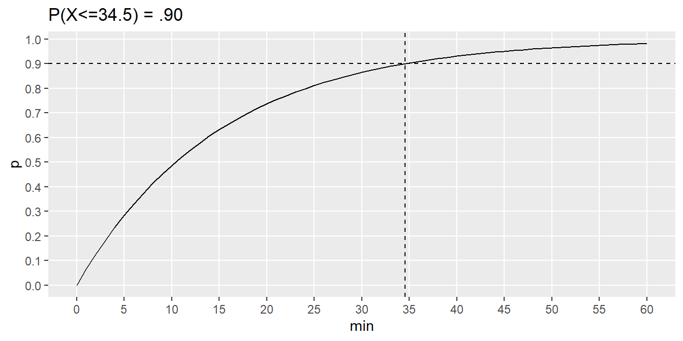

The average time for two buses to arrive is \(2 \cdot E[X] = 2 \cdot \frac{1}{1/15} = 30\) minutes.