2.6 Gamma

Gamma distributions are usually used to model wait times until events. Unlike the exponential distribution which models the time until the first event, gamma models the time until the \(\alpha\)th or \(k\)th event.

Before you learn about the gamma distribution, you should understand the gamma function, \(\Gamma(n) = (n-1)!\), because it is part of the definition. \(\Gamma(n)\) extends the factorial from nonnegative whole numbers to a subset of the real numbers. The generalization of the factorial is used in combinatorics and probability problems. Some probability distributions are defined in terms of the gamma function, including the student t, chi-square, and gamma distribution.

The gamma distribution is a two-parameter distribution. You will encounter two forms of the gamma distribution.

• shape \(k\) and scale \(\theta\).
• shape \(\alpha = k\) and rate \(\beta = 1/\theta\).

The probability density function for the shape \(k\) and scale \(\theta\) form is

If \(X\) is the interval until the \(k^{th}\) successful event when the average interval is \(\theta\), then \(X\) is a random variable with a gamma distribution \(X \sim \mathrm{\Gamma}(\alpha, \theta)\). The probability of an interval of \(X = x\) is

\[f(x; k, \theta) = \frac{x^{k-1} e^{-\frac{x}{\theta}}}{\theta^k \Gamma(k)} \hspace{1cm} x, k, \theta > 0.\]

with \(E(X) = k \theta\) and variance \(Var(X) = k \theta^2\).

The probability density function for the shape \(\alpha\) and rate \(\beta\) form is

If \(X\) is the interval until the \(\alpha^{th}\) successful event when events occur at a rate of \(\beta\) times per interval, then \(X\) is a random variable with a gamma distribution \(X \sim \mathrm{\Gamma}(k, \beta)\). The probability of an interval of \(X = x\) is

\[f(x; \alpha, \beta) = \frac{\beta^\alpha x^{\alpha-1}e^{-\beta x}}{\Gamma(k)} \hspace{1cm} x, \alpha, \beta > 0.\]

with \(E(X) = \alpha / \beta\) and variance \(Var(X) = \alpha / \beta^2\).

Gamma is the conjugate prior to the Poisson, exponential, normal, Pareto, and gamma likelihood distributions.

Example. On average, someone sends a money order once per 15 minutes (\(\theta = .25\)). What is the probability someone sends \(k = 10\) money orders in less than \(x = 3\) hours?* This is a shape/scale formulation.

pgamma(q = 3, shape = 10, scale = 0.25)
## [1] 0.7576078

You could equally express it in a shape/rate formulation by saying “4 money orders are sent per hour.”

pgamma(q = 3, shape = 10, scale = 1 / 4)
## [1] 0.7576078

data.frame(x = 0:1000 / 100) %>%
  mutate(prob = pgamma(q = x, shape = 10, scale = .25, lower.tail = TRUE)) %>%
ggplot(aes(x = x, y = prob)) +
  geom_line() +
  geom_vline(xintercept = 3, linetype = 2) +
  geom_hline(yintercept = pgamma(3, shape = 10, scale = .25), linetype = 2) +
  scale_x_continuous(breaks = 0:10) +
  theme(panel.grid.minor = element_blank()) +
  labs(title = "P(X = 3, alpha = 10, theta = .25) = .758",
       subtitle = "Probability of 10 events in 3 hours when the mean time to event is .25 hours.",
       x = "Interval (x) (hours)",
       y = "pgamma")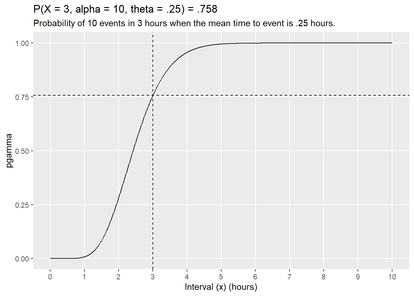 

References: Arein Kim.