2.2 Binomial
Binomial sampling is used to model counts of one level of a categorical variable over a fixed sample size.
If \(X\) is the count of successful events in \(n\) identical and independent Bernoulli trials of success probability \(\pi\), then \(X\) is a random variable with a binomial distribution \(X \sim \mathrm{Bin}(n,\pi)\)
\[f(X = k;n, \pi) = \frac{n!}{k!(n-k)!} \pi^k (1-\pi)^{n-k} \hspace{1cm} k \in (0, 1, ..., n), \hspace{2mm} \pi \in [0, 1]\]
with \(E(X)=n\pi\) and \(Var(X) = n\pi(1-\pi)\).
Consider a data set dat_bin containing frequencies of high-risk drinkers vs non-high-risk drinkers in a college survey.
dat_bin <- data.frame(
  subject = 1:1315,
  high_risk = factor(c(rep("Yes", 630), rep("No", 685)))
)
janitor::tabyl(dat_bin$high_risk)
## dat_bin$high_risk n percent
## No 685 0.5209125
## Yes 630 0.4790875The MLE of \(\pi\) from the Binomial distribution is the sample mean.
x <- sum(dat_bin$high_risk == "Yes")
n <- nrow(dat_bin)
p <- x / n
print(p)
## [1] 0.4790875data.frame(events = seq(550, 700, 10),
pmf = dbinom(seq(550, 700, 10), n, p),
cdf = pbinom(seq(550, 700, 10), n, p, lower.tail = TRUE)) %>%
ggplot() +
geom_col(aes(x = events, y = pmf)) +
geom_text(aes(x = events, label = round(pmf, 3), y = pmf + 0.001),
position = position_dodge(0.9), size = 3, vjust = 0) +
geom_line(aes(x = events, y = cdf/40), size = 1) +
scale_y_continuous(limits = c(0, .025),
sec.axis = sec_axis(~ . * 40, name = "Cum Prob")) +
labs(title = "PMF and CDF of Binomial Distribution",
subtitle = paste0("Bin(", n, ", ", scales::comma(p, accuracy = .01), ")"),
x = "X = k", y = "Density")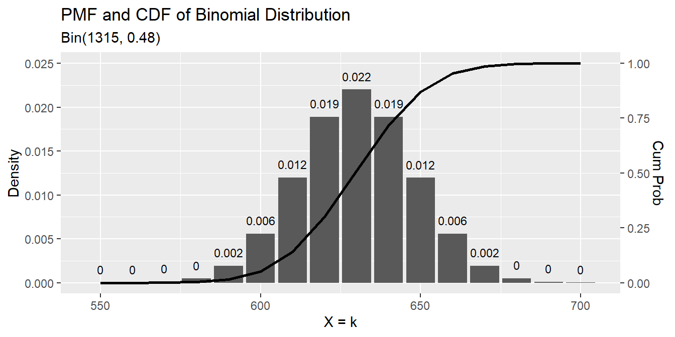
There are several ways to calculate a 95% CI for \(\pi\). One method is the normal approximation Wald interval.
\[\pi = p \pm z_{\alpha /2} \sqrt{\frac{p (1 - p)}{n}}\]
z <- qnorm(.975)
se <- sqrt(p * (1 - p) / n)
p + c(-z*se, z*se)
## [1] 0.4520868 0.5060882The Wald interval’s accuracy suffers when \(np<5\) or \(n(1-p)<5\) and it does not work at all when \(p = 0\) or \(p = 1\). Option two is the Wilson method.
\[\frac{p + \frac{z^2}{2n}}{1 + \frac{z^2}{n}} \pm \frac{z}{1 + \frac{z^2}{n}} \sqrt{\frac{p(1 - p)}{n} + \frac{z^2}{4n^2}}\]
est <- (p + (z^2)/(2*n)) / (1 + (z^2) / n)
pm <- z / (1 + (z^2)/n) * sqrt(p*(1-p)/n + (z^2) / (4*(n^2)))
est + c(-pm, pm)
## [1] 0.4521869 0.5061098This is what prop.test(correct = FALSE) calculates.
prop.test(x = x, n = n, correct = FALSE)##
## 1-sample proportions test without continuity correction
##
## data: x out of n, null probability 0.5
## X-squared = 2.3004, df = 1, p-value = 0.1293
## alternative hypothesis: true p is not equal to 0.5
## 95 percent confidence interval:
## 0.4521869 0.5061098
## sample estimates:
## p
## 0.4790875There is a second version of the Wilson interval that applies a “continuity correction” that aligns the “minimum coverage probability,” rather than the “average probability,” with the nominal value.
prop.test(x = x, n = n)##
## 1-sample proportions test with continuity correction
##
## data: x out of n, null probability 0.5
## X-squared = 2.2175, df = 1, p-value = 0.1365
## alternative hypothesis: true p is not equal to 0.5
## 95 percent confidence interval:
## 0.4518087 0.5064898
## sample estimates:
## p
## 0.4790875Finally, there is the Clopper-Pearson exact confidence interval. Clopper-Pearson inverts two single-tailed binomial tests at the desired alpha. This is a non-trivial calculation, so there is no easy formula to crank through. Just use the binom.test() function and pray no one asks for an explanation.
binom.test(x = x, n = n)##
## Exact binomial test
##
## data: x and n
## number of successes = 630, number of trials = 1315, p-value = 0.1364
## alternative hypothesis: true probability of success is not equal to 0.5
## 95 percent confidence interval:
## 0.4517790 0.5064896
## sample estimates:
## probability of success
## 0.4790875The expected probability of no one being a high-risk drinker is \(f(0;0.479) = \frac{1315!}{0!(1315-0)!} 0.479^0 (1-0.479)^{1315-0} = 0\). Use dbinom() for probability densities.
dbinom(x = 0, size = n, p = p)
## [1] 0
The expected probability of at least half the population being a high-risk drinker, \(f(658, 0.479) = .065\). Use pbinom() for cumulative probabilities.
pbinom(q = .5*n, size = n, prob = p, lower.tail = FALSE)
## [1] 0.06455096
The normal distribution is a good approximation when \(n\) is large. The \(\lim_{n \rightarrow \infty} \mathrm{Bin}(n, \pi) = N(n\pi, n\pi(1−\pi)).\)
pnorm(q = 0.5, mean = p, sd = se, lower.tail = FALSE)
## [1] 0.06450357
Suppose a second survey gets a slightly different result. The high risk = Yes falls from 630 (48%) to 600 (46%).
dat_bin2 <- data.frame(
  subject = 1:1315,
  high_risk = factor(c(rep("Yes", 600), rep("No", 715)))
)
(dat2_tabyl <- janitor::tabyl(dat_bin2, high_risk))
## high_risk n percent
## No 715 0.5437262
## Yes 600 0.4562738The two survey counts of high risk = “Yes” are independent random variables distributed \(X \sim \mathrm{Bin}(1315, .48)\) and \(Y \sim \mathrm{Bin}(1315, .46)\). What is the probability that either variable is \(X \ge 650\)?
Let \(P(A) = P(X \le 650)\) and \(P(B) = P(Y \le 650)\). Then \(P(A|B) = P(A) + P(B) - P(AB)\), and because the events are independent, \(P(AB) = P(A)P(B)\).
(p_a <- pbinom(q = 650, size = 1315, prob = 0.48, lower.tail = FALSE))
## [1] 0.1433791
(p_b <- pbinom(q = 650, size = 1315, prob = 0.46, lower.tail = FALSE))
## [1] 0.005868366
(p_a + p_b - (p_a * p_b))
## [1] 0.1484061
Here’s an empirical test.
df <- data.frame(
  x = rbinom(10000, 1315, 0.48),
  y = rbinom(10000, 1315, 0.46)
  )
mean(if_else(df$x >= 650 | df$y >= 650, 1, 0))
## [1] 0.1624A couple other points to remember:
- The Bernoulli distribution is a special case of the binomial with \(n = 1\).
- The binomial distribution assumes independent trials. If you sample without replacement from a finite population, use the hypergeometric distribution.