2.7 Beta
The beta distribution, \(\mathrm{Beta}(\alpha, \beta)\), is a family of distributions used to model probabilities. In Bayesian inference, it is frequently the conjugate prior distribution for the Bernoulli, binomial, negative binomial, and geometric distributions. When the beta distribution is used as the conjugate prior, the posterior distribution is also a beta distribution, greatly reducing the complexity of the analysis. After accumulating additional evidence, you simply adjust the \(\alpha\) and \(\beta\) parameters.
If \(P\) is the probability of success in a random process then \(P\) may be expressed as a random variable with a beta distribution \(P \sim \mathrm{Beta}(\alpha, \beta)\). The probability that \(P = p\) is
\[f(p; \alpha, \beta) = \frac{p^{\alpha-1} (1-p)^{\beta-1}}{\mathrm{B}(\alpha, \beta)}, \hspace{1cm} \mathrm{B}(\alpha, \beta) = \frac{\Gamma(\alpha) \Gamma(\beta)}{\Gamma(\alpha + \beta)}.\]
with \(E(X) = \frac{\alpha}{\alpha + \beta}\).
The \(\mathrm{B}(\alpha, \beta)\) is a normalization constant that causes the pdf to integrate to 1 over the range of \(p\), \(\int_0^1f(p)dp = 1.\)
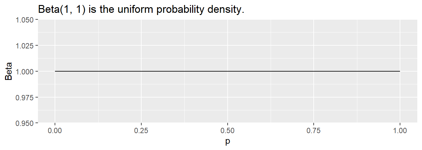
\(\mathrm{Beta}(1, 1)\) expresses a uniform probability density, the expression of complete ignorance of the correct prior distribution.
data.frame(p = seq(0, 1, .01)) %>%
  mutate(Beta = dbeta(p, 1, 1)) %>%
  ggplot(aes(x = p, y = Beta)) +
  geom_line() +
  labs(title = "Beta(1, 1) is the uniform probability density.")
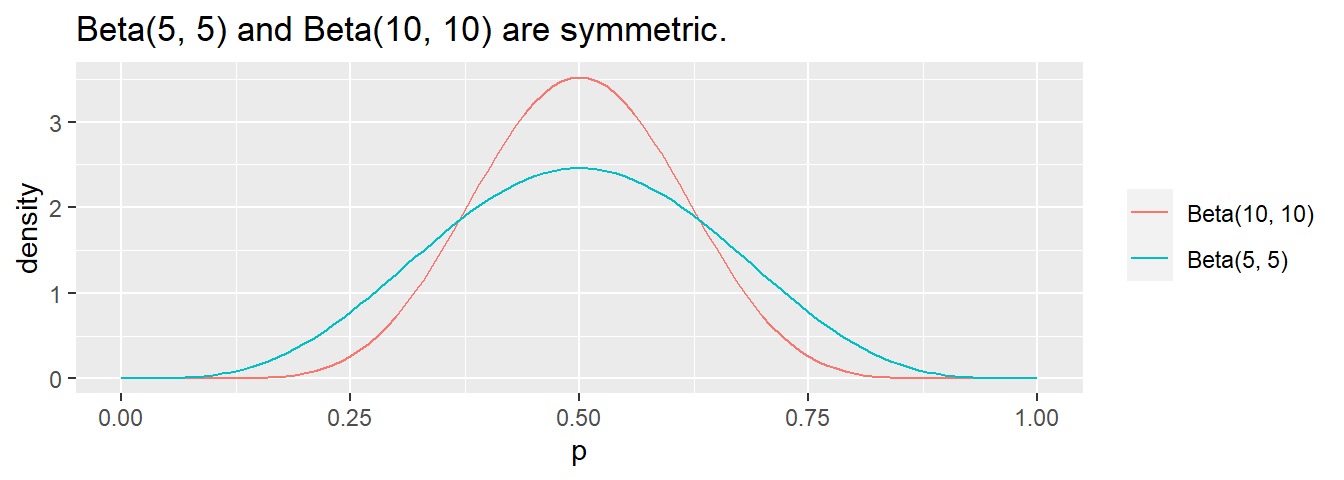
\(\mathrm{Beta}(5, 5)\) is a symmetric probability; \(\mathrm{Beta}(10, 10)\) is also symmetric, but with smaller variance. In general, the strength of the prior increases with the sum of \(\alpha + \beta\).

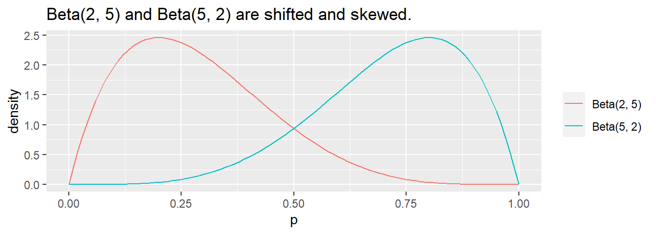
The distribution shifts to the left if \(\beta\) > \(\alpha\) and right if \(\alpha\) > \(\beta\).

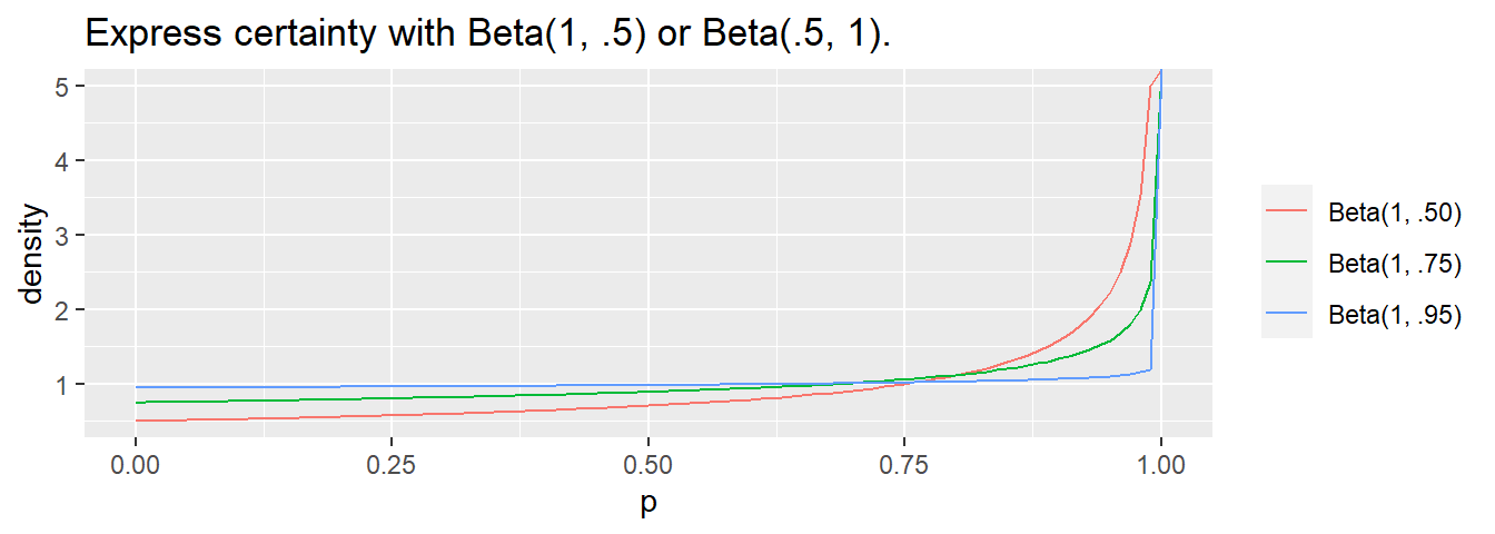
If one of the values is < 1, the curve flips toward \(\infty\) at the extreme. \(\alpha\) or \(\beta\) is usually 0.5 to denote near certainty.
