Chapter 3 Plant Height
3.1 2019 Plant Height Data
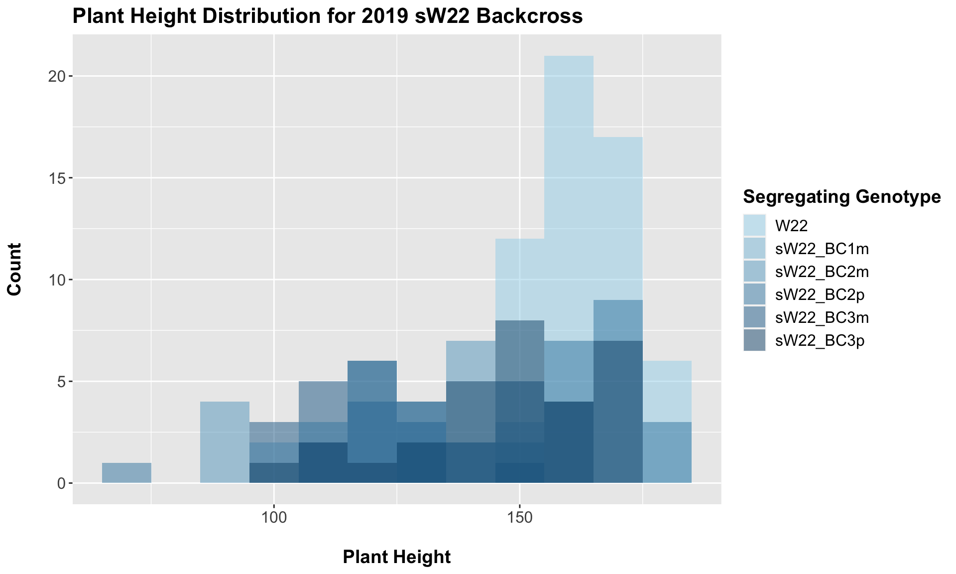
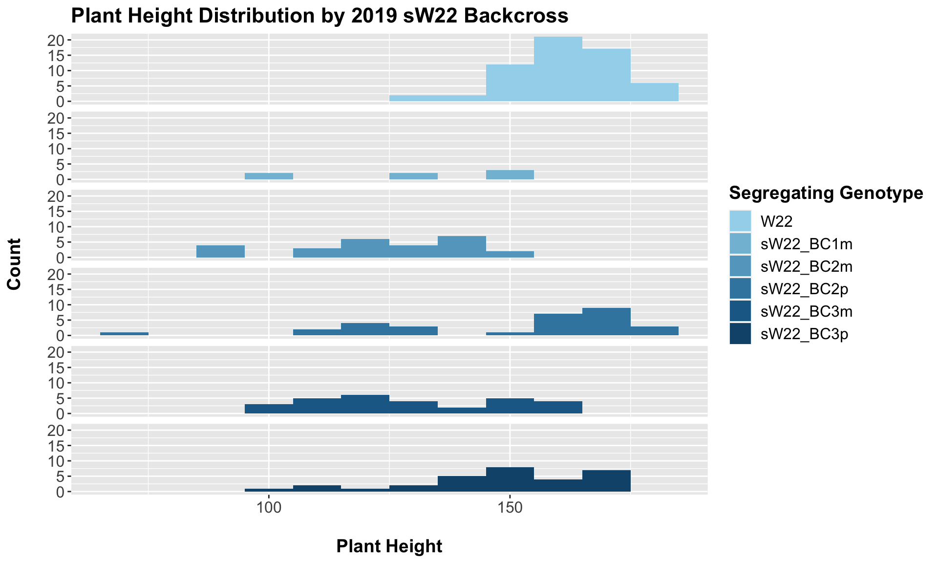
3.1.1 2019 sW22 backcrossed to W22
##
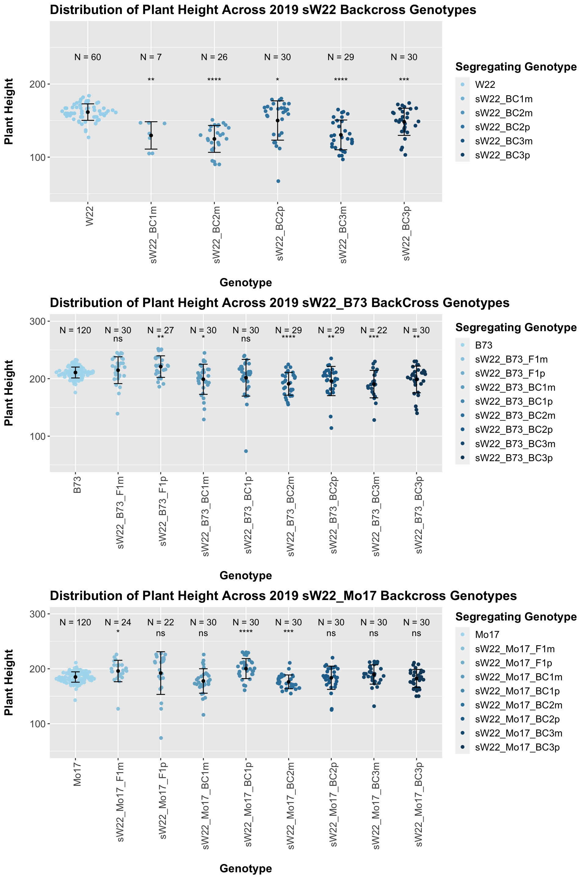
## Mean, SD, and SE for each genotype## Seg_Genotype N mean sd se
## 1 W22 60 161.6167 11.28835 1.457320
## 2 sW22_BC1m 7 129.7143 18.72355 7.076838
## 3 sW22_BC2m 26 124.9231 18.36937 3.602530
## 4 sW22_BC2p 30 150.1000 26.87692 4.907032
## 5 sW22_BC3m 29 130.4138 20.36369 3.781442
## 6 sW22_BC3p 30 148.3000 18.55123 3.386976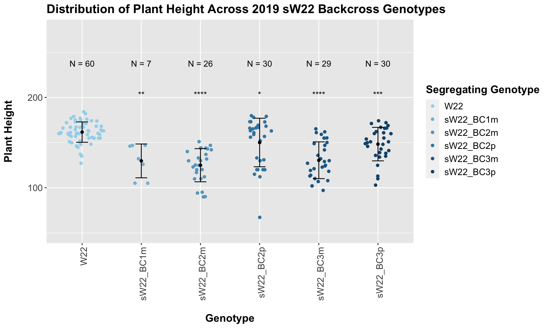
##
## Results of T-test used to obtain significance in the above plot
## # A tibble: 5 x 8
## .y. group1 group2 p p.adj p.format p.signif method
## <chr> <chr> <chr> <dbl> <dbl> <chr> <chr> <chr>
## 1 Plant_Height W22 sW22_BC1m 3.68e- 3 7.40e- 3 0.00368 ** T-test
## 2 Plant_Height W22 sW22_BC2m 5.80e-11 2.90e-10 5.8e-11 **** T-test
## 3 Plant_Height W22 sW22_BC2p 3.10e- 2 3.10e- 2 0.03100 * T-test
## 4 Plant_Height W22 sW22_BC3m 3.67e- 9 1.50e- 8 3.7e-09 **** T-test
## 5 Plant_Height W22 sW22_BC3p 8.38e- 4 2.50e- 3 0.00084 *** T-testFrom this, we can see a distinct reduction in plant height among the backcrosses compared to the W22 control. BC1m not only shows reduced stature but also notably fewer data points (could this mean that fewer BC1m plants reached maturity in order to collect plant height information?). When we have comparisons between the sick plant being either the maternal or paternal parent, it does seem like the paternal lineage is a bit taller? From our 2020 data, we only had one maternal/paternal comaprison (BC2), and I did not see a noticeable difference between the two.
We may also we separate the data by which field the row was in.
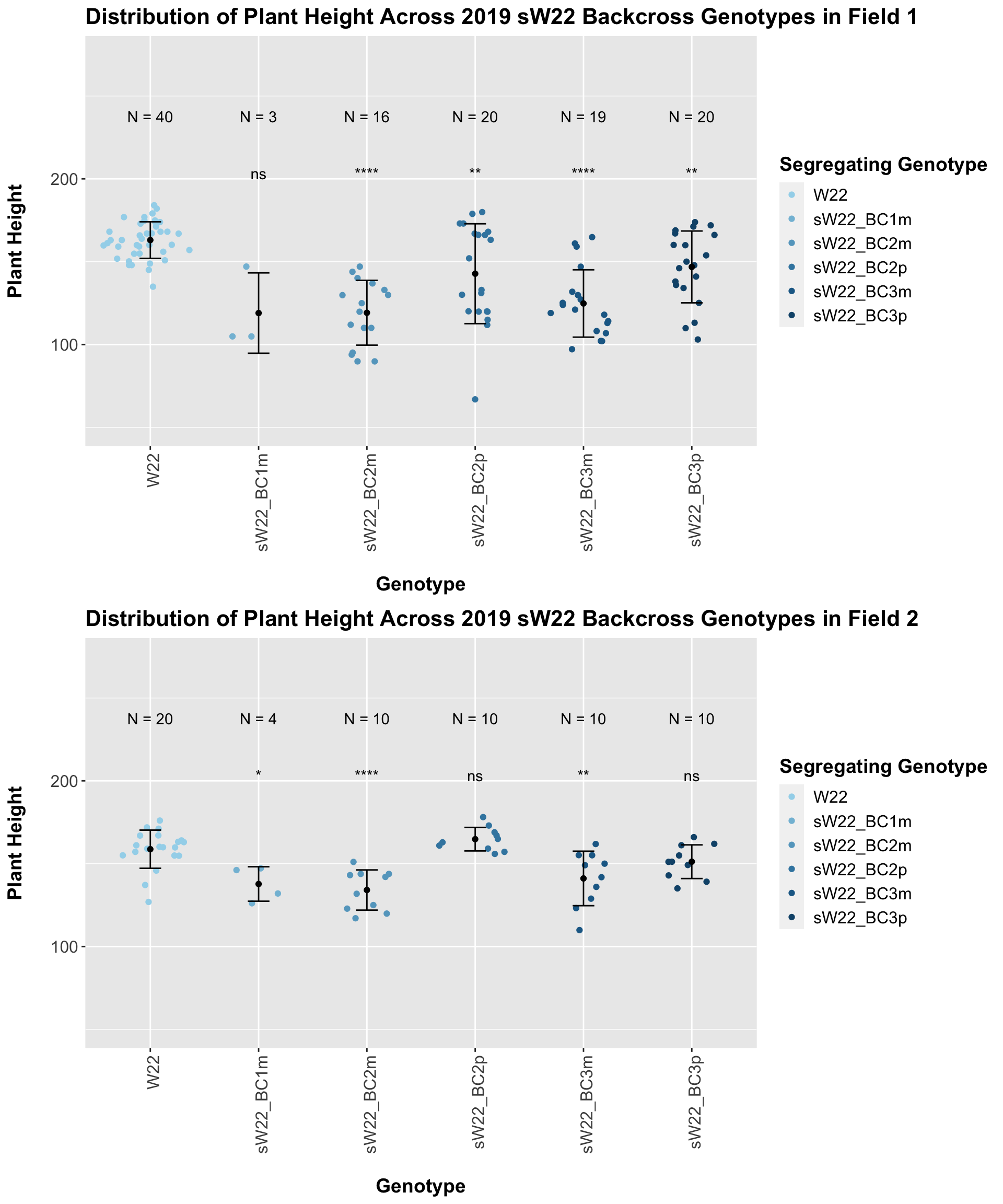
Our results seem equally, if not more, significant once separated by field, particularly in Field 1. The trend seems to be similar to that of the 2020 sW22 backcrosses.
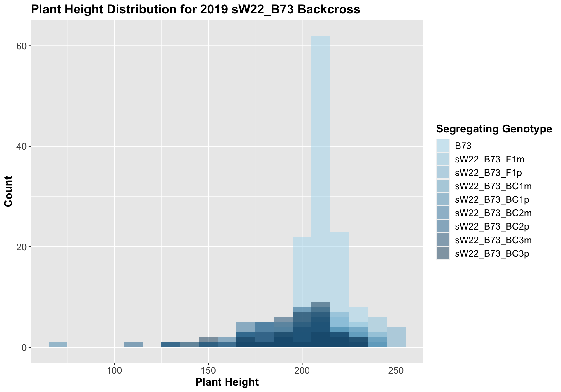
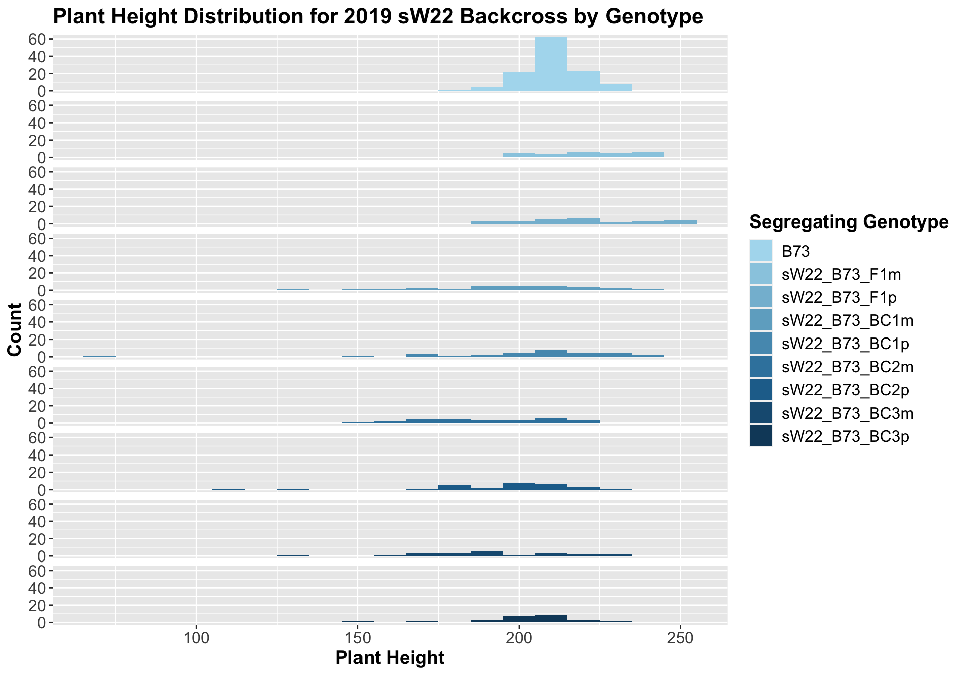
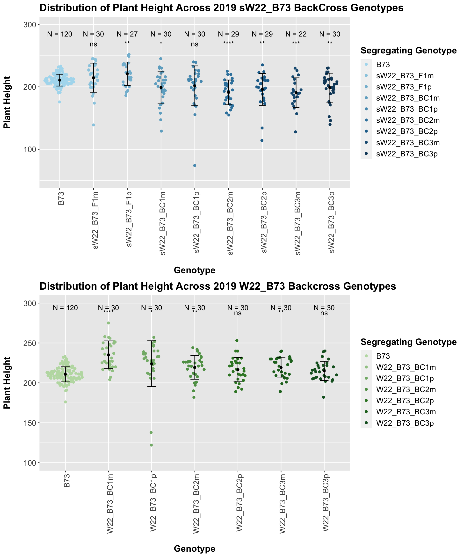
3.1.2 2019 sW22 and W22 backcrossed to B73
##
##  Mean, SD, and SE for each genotype
## Seg_Genotype N mean sd se
## 1 B73 120 210.7167 9.459496 0.8635299
## 2 sW22_B73_F1m 30 214.7333 23.322231 4.2580373
## 3 sW22_B73_F1p 27 221.0000 18.724727 3.6035753
## 4 sW22_B73_BC1m 30 198.9333 26.192830 4.7821347
## 5 sW22_B73_BC1p 30 201.6000 31.924048 5.8285070
## 6 sW22_B73_BC2m 29 191.0690 19.849309 3.6859242
## 7 sW22_B73_BC2p 29 195.8966 25.432466 4.7226904
## 8 sW22_B73_BC3m 22 190.5455 23.880112 5.0912569
## 9 sW22_B73_BC3p 30 198.6667 23.219096 4.2392076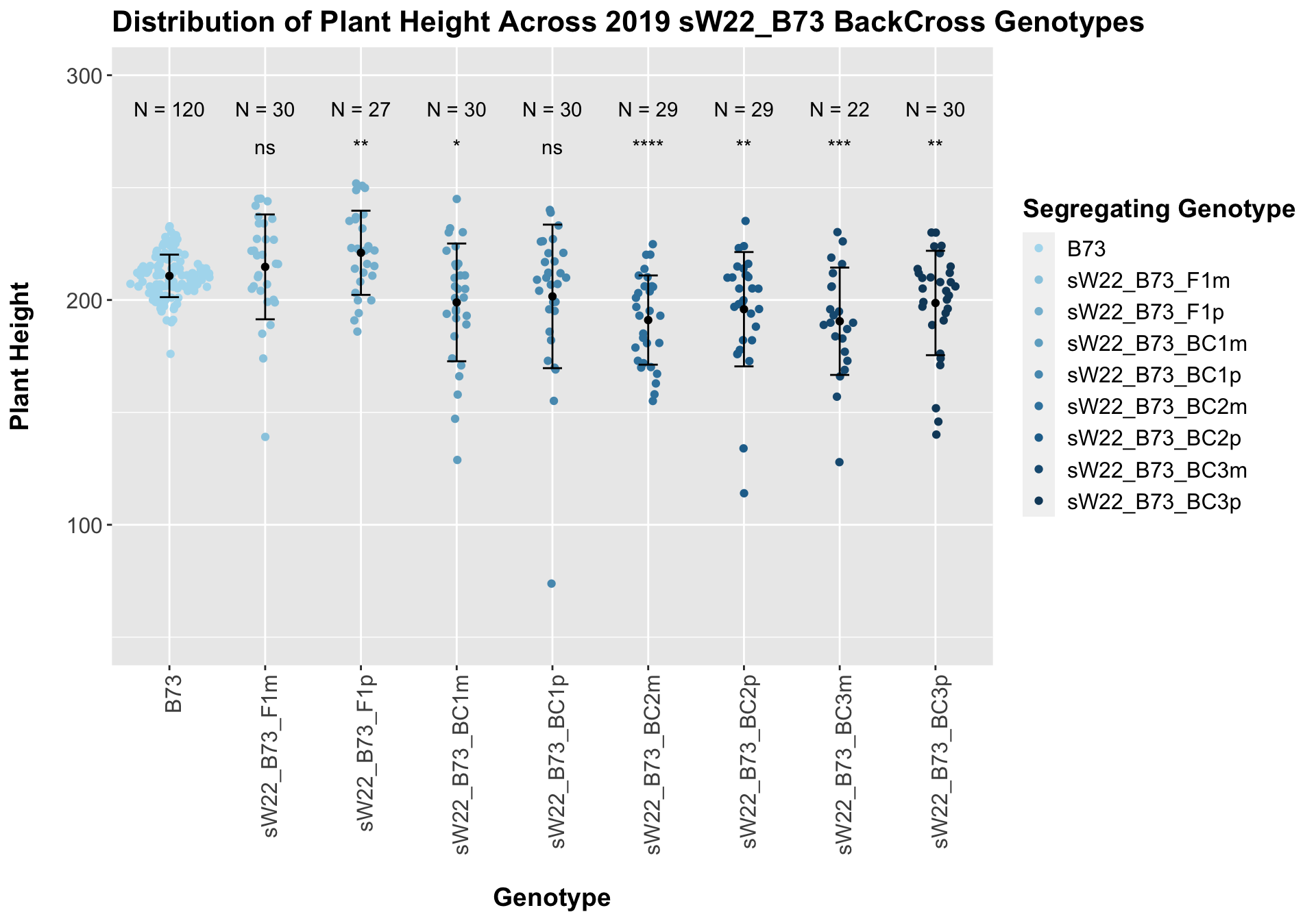
## # A tibble: 8 x 8
##   .y.          group1 group2                p    p.adj p.format p.signif method
##   <chr>        <chr>  <chr>             <dbl>    <dbl> <chr>    <chr>    <chr>
## 1 Plant_Height B73    sW22_B73_F1m  0.362     0.36     0.36227  ns       T-test
## 2 Plant_Height B73    sW22_B73_F1p  0.00955   0.045    0.00955  **       T-test
## 3 Plant_Height B73    sW22_B73_BC1m 0.0214    0.064    0.02135  *        T-test
## 4 Plant_Height B73    sW22_B73_BC1p 0.132     0.26     0.13219  ns       T-test
## 5 Plant_Height B73    sW22_B73_BC2m 0.0000123 0.000098 1.2e-05  ****     T-test
## 6 Plant_Height B73    sW22_B73_BC2p 0.00434   0.026    0.00434  **       T-test
## 7 Plant_Height B73    sW22_B73_BC3m 0.000747  0.0052   0.00075  ***      T-test
## 8 Plant_Height B73    sW22_B73_BC3p 0.00898   0.045    0.00898  **       T-test
Here, we see a small increase in plant height for the initial F1s. As we continue backcrossing to B73, we see a decline in plant height. The shape across the generations is less pronounced though than in the 2020 sW22_B73 backcrosses. Once, again, we separate the data by field, to see whether the trend is the same.
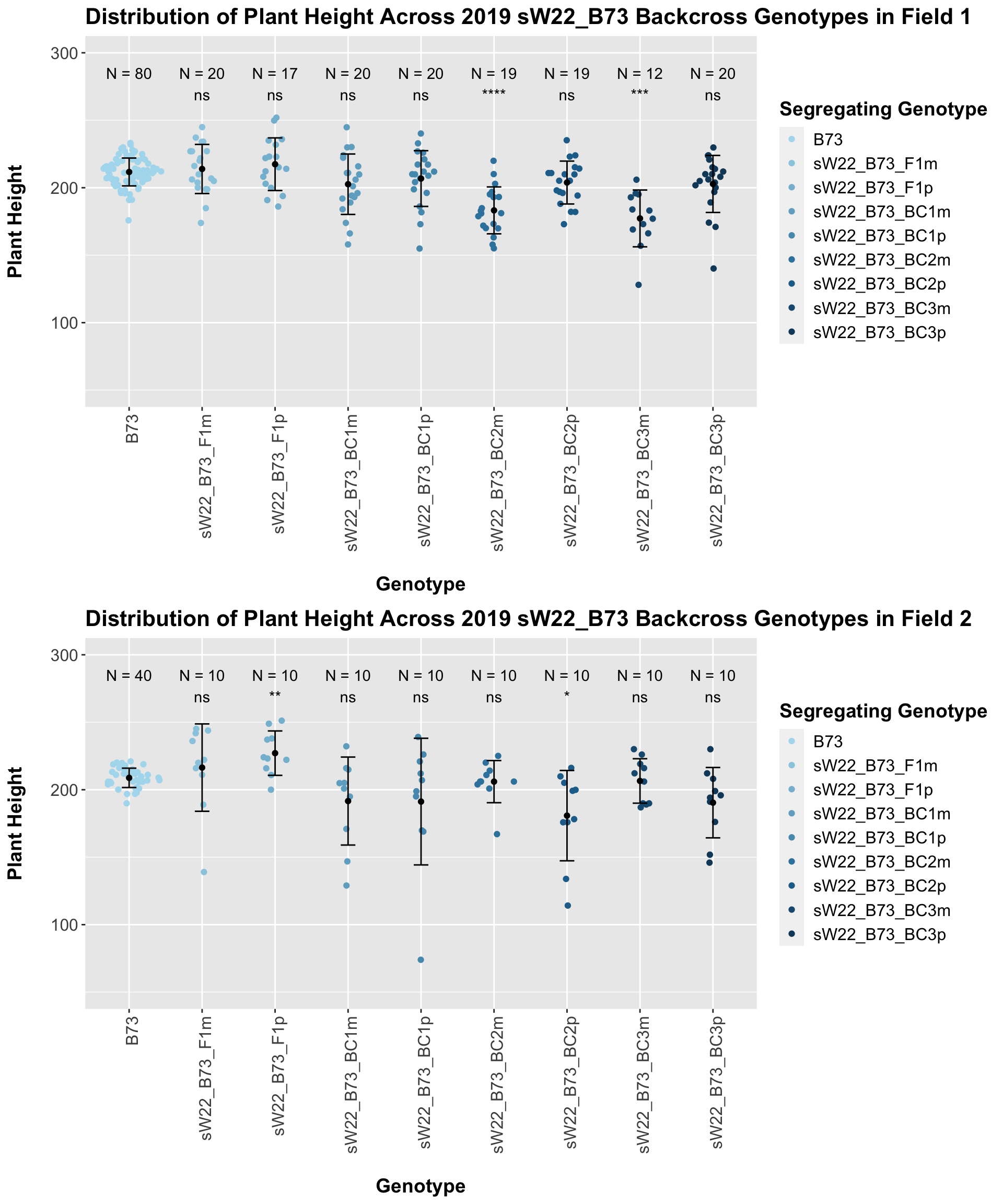
If we separate by field, we lose almost all significance when comparing backcrosses to the B73 line. This is notably different from the data seen in 2020. We can compare the height data across the W22 backcrossed to B73 rows to look at this set of controls.
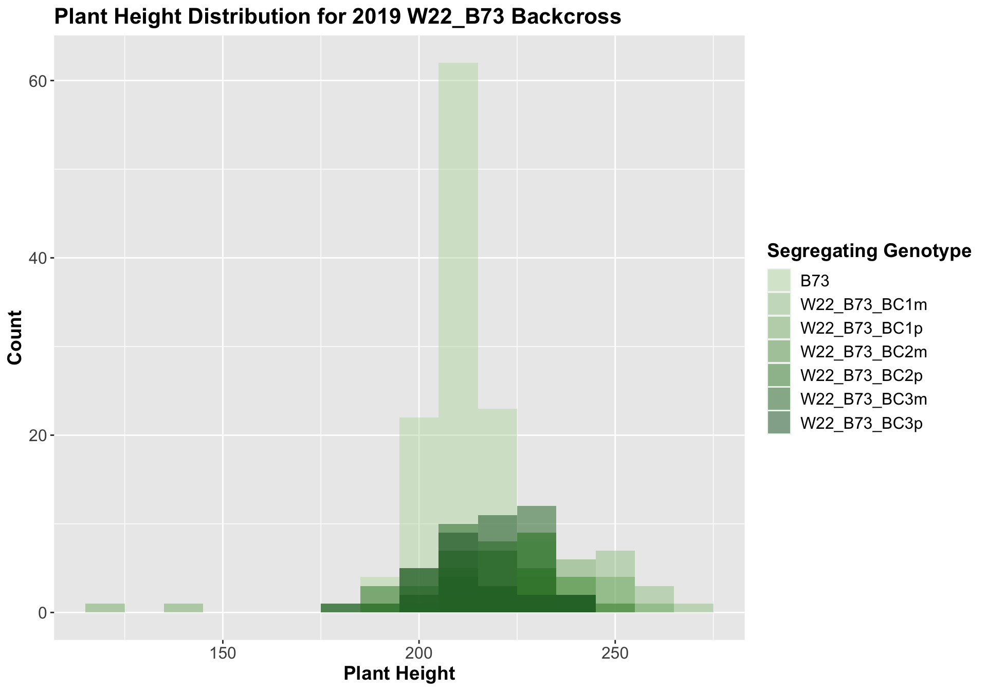
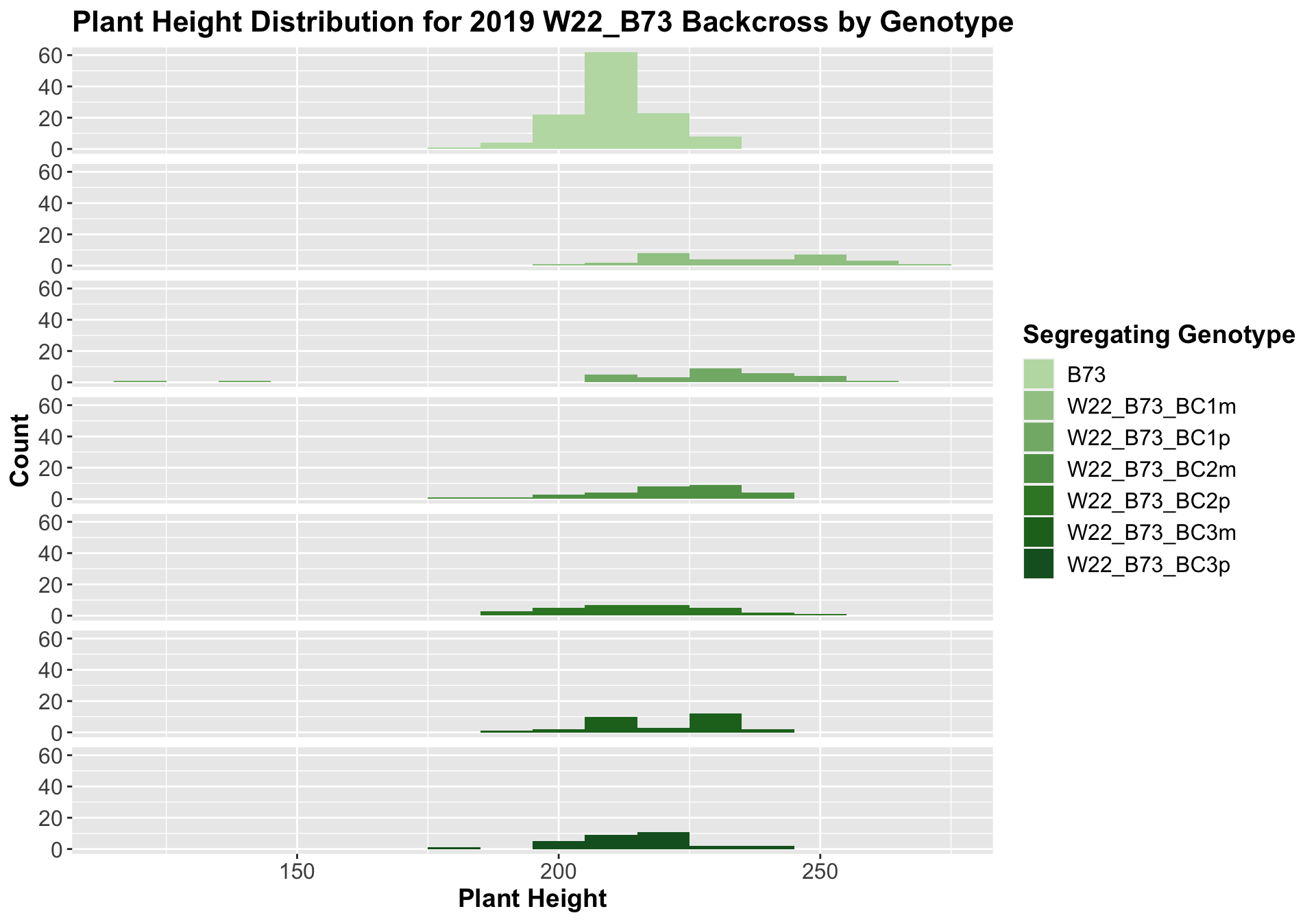
##
##  Mean, SD, and SE for each genotype
## Seg_Genotype N mean sd se
## 1 B73 120 210.7167 9.459496 0.8635299
## 2 W22_B73_BC1m 30 235.2333 17.383471 3.1737730
## 3 W22_B73_BC1p 30 224.0000 28.742615 5.2476596
## 4 W22_B73_BC2m 30 219.5333 14.947571 2.7290406
## 5 W22_B73_BC2p 30 216.5000 15.133316 2.7629528
## 6 W22_B73_BC3m 30 219.2000 12.981153 2.3700235
## 7 W22_B73_BC3p 30 215.0000 12.071625 2.2039672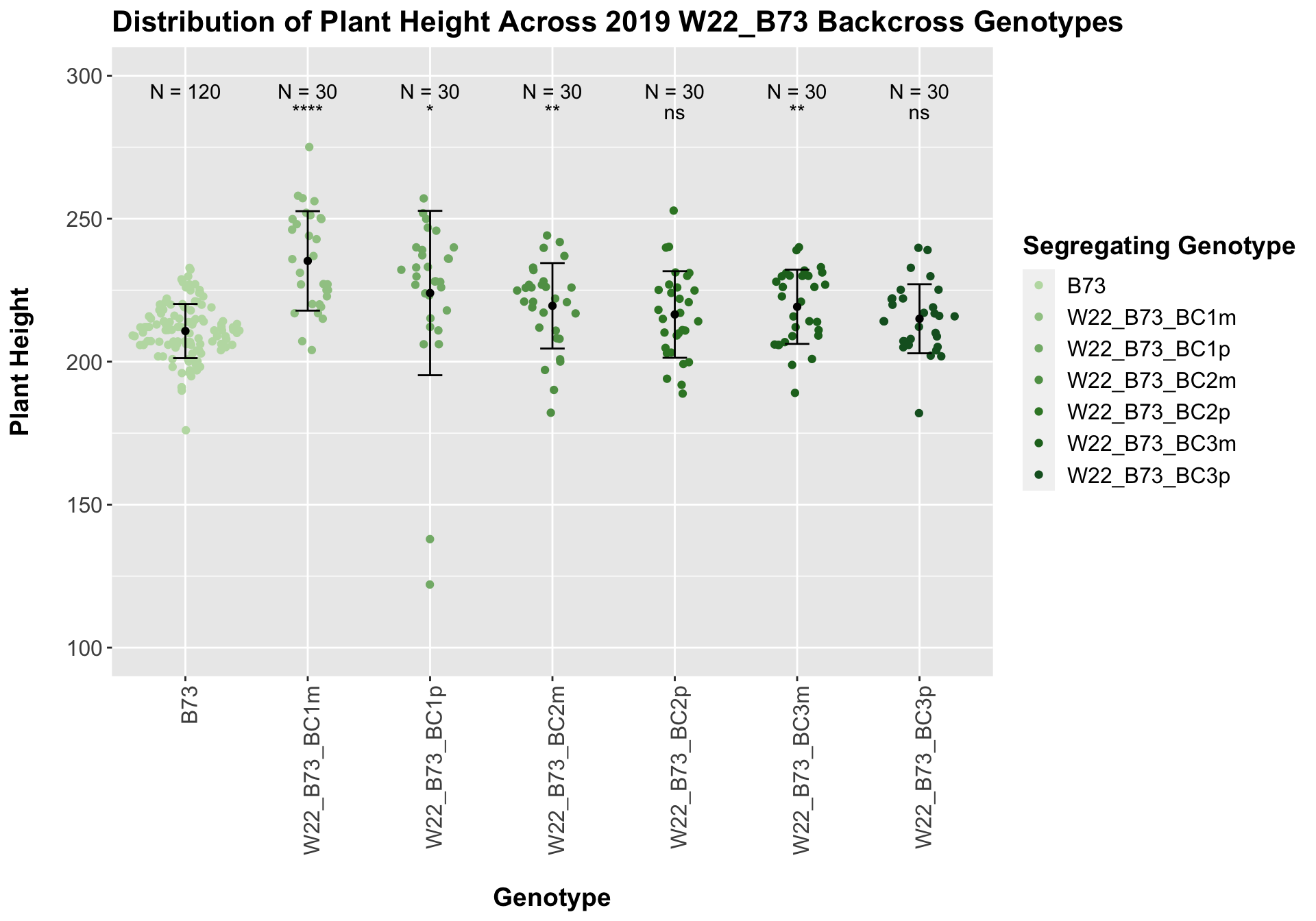
## # A tibble: 6 x 8
##   .y.         group1 group2                 p     p.adj p.format p.signif method
##   <chr>       <chr>  <chr>              <dbl>     <dbl> <chr>    <chr>    <chr>
## 1 Plant_Heig… B73    W22_B73_BC1m     1.34e-8   8.00e-8 1.3e-08  ****     T-test
## 2 Plant_Heig… B73    W22_B73_BC1p     1.81e-2   5.40e-2 0.0181   *        T-test
## 3 Plant_Heig… B73    W22_B73_BC2m     4.01e-3   1.60e-2 0.0040   **       T-test
## 4 Plant_Heig… B73    W22_B73_BC2p     5.36e-2   1.10e-1 0.0536   ns       T-test
## 5 Plant_Heig… B73    W22_B73_BC3m     1.80e-3   9.00e-3 0.0018   **       T-test
## 6 Plant_Heig… B73    W22_B73_BC3p     7.82e-2   1.10e-1 0.0782   ns       T-test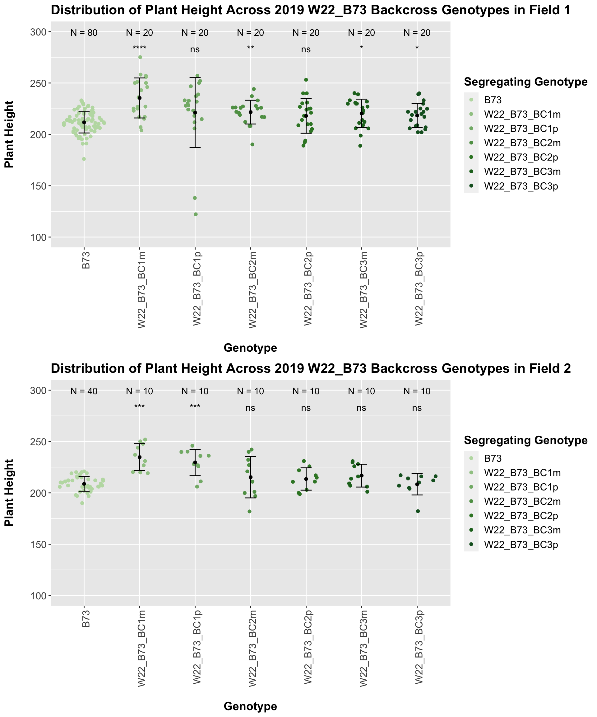
Once again, we see an initial increase in plant height among our backcrosses that slowly declines. This pattern holds if we separate by field, but, once again, the difference between the W22 backcross and the B73 line becomes marginal/nonsignificant.
We may also compare the distribution for sW22_B73 backcrosses to W22_B73 backcrosses and each generation compares across these two sets. Note: when looking at these plots, just be aware that the genotypes don't align perfectly across backcrosses because we don't have a few crosses for the W22_B73 genotypes.
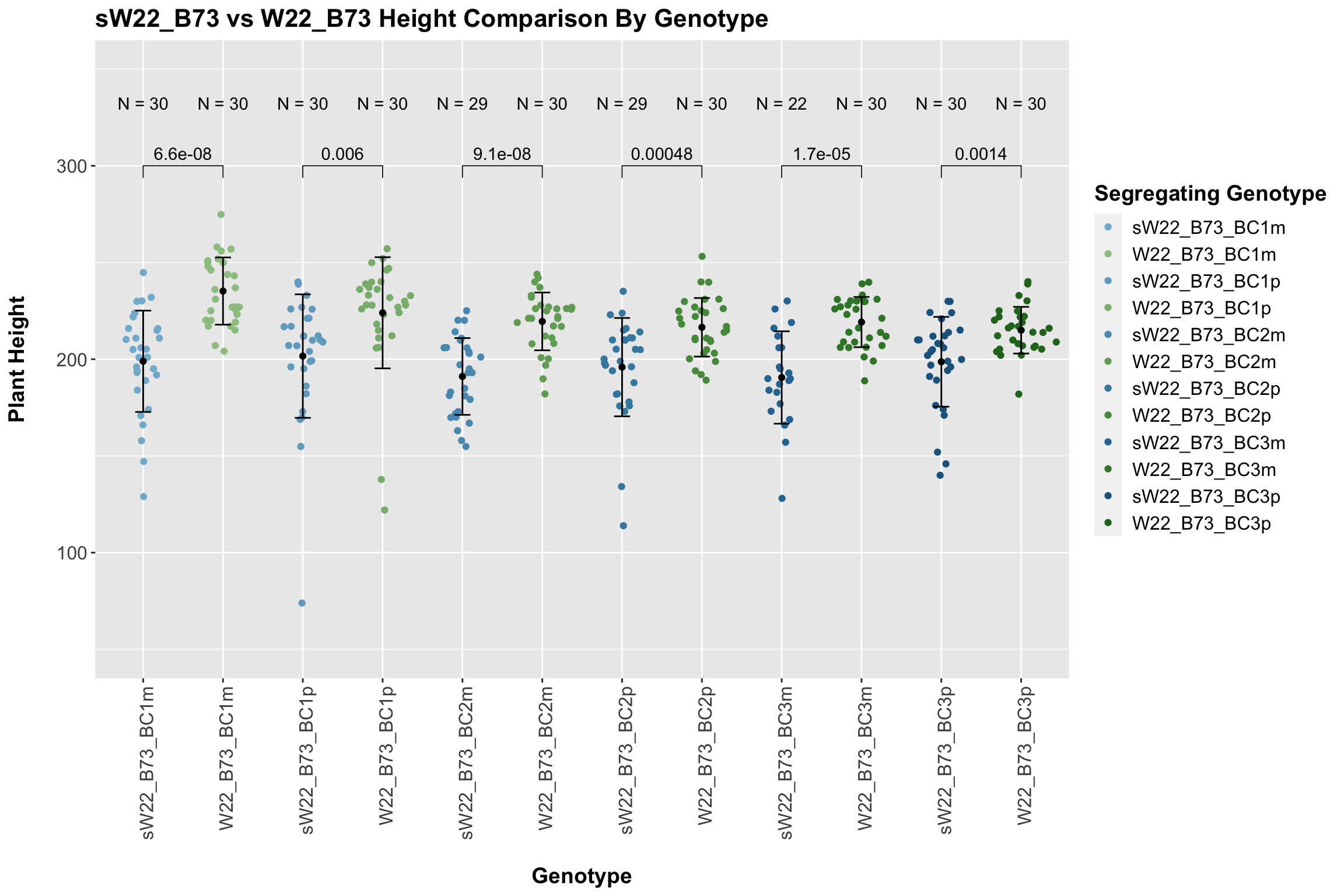
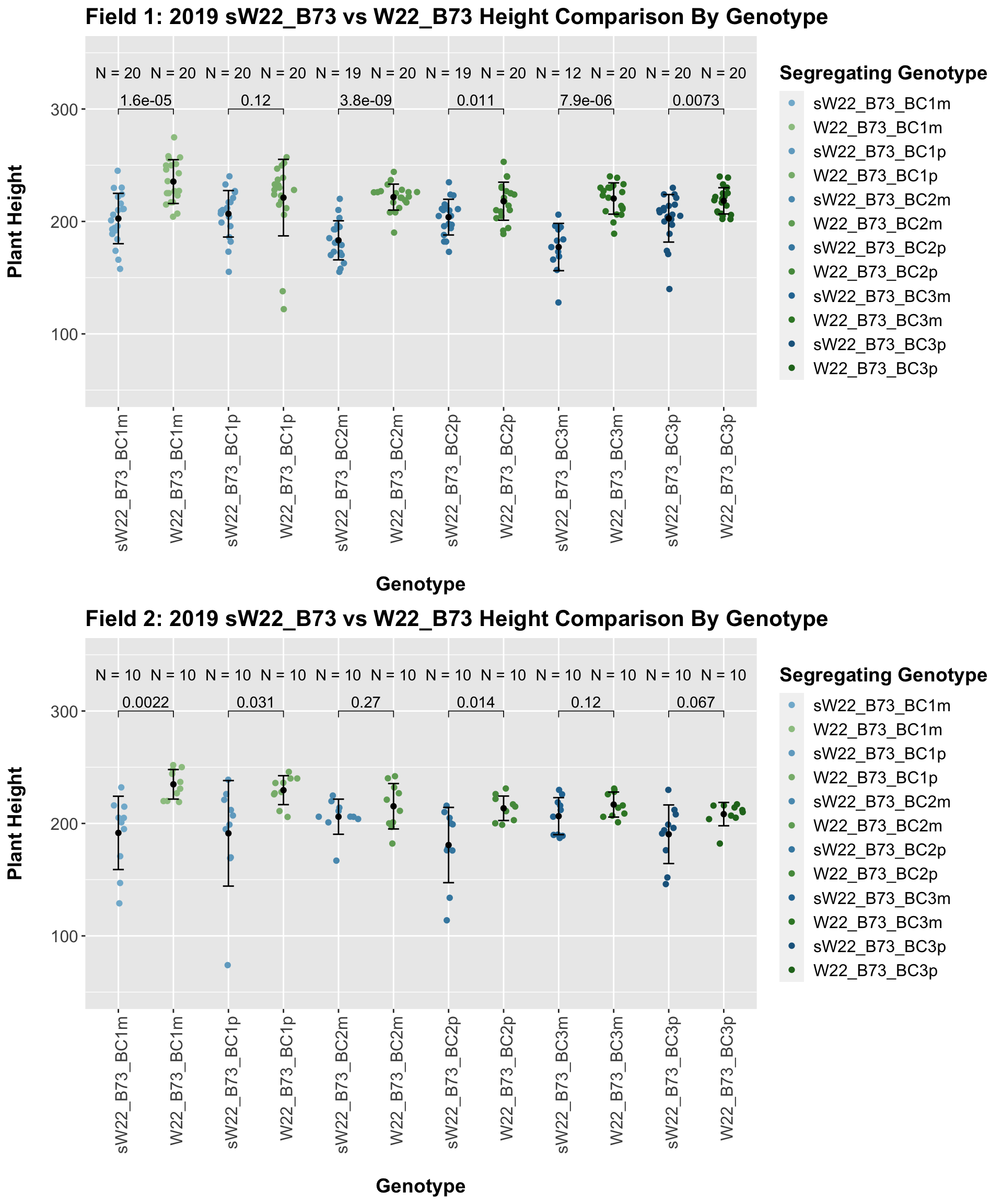
When we specifically compare the height between sW22 and W22 backcrossed to B73 at each generation, we see a significant reduction in height of the sW22 backcross against the W22 backcross. However, if we stratify this data by field, we see that this trend does not seem to hold signifciance in field 2.
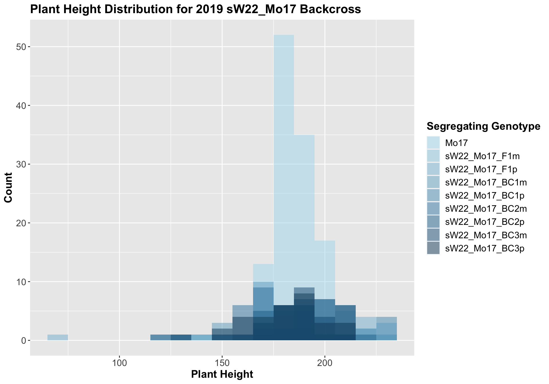
3.1.3 2019 sW22 and W22 backcrossed to Mo17
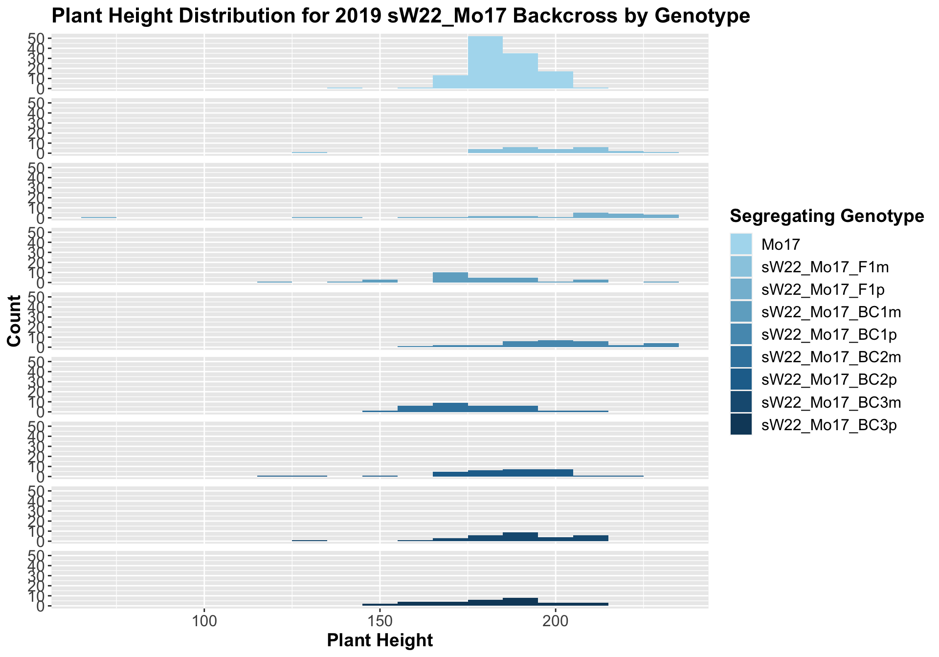
##
##  Mean, SD, and SE for each genotype
## Seg_Genotype N mean sd se
## 1 Mo17 120 185.0250 9.441961 0.8619292
## 2 sW22_Mo17_F1m 24 195.9583 19.550335 3.9906953
## 3 sW22_Mo17_F1p 22 192.1818 38.863174 8.2856566
## 4 sW22_Mo17_BC1m 30 177.8000 22.274773 4.0667986
## 5 sW22_Mo17_BC1p 30 200.3333 18.253641 3.3326436
## 6 sW22_Mo17_BC2m 30 176.2000 12.581870 2.2971246
## 7 sW22_Mo17_BC2p 30 183.6333 21.170056 3.8651057
## 8 sW22_Mo17_BC3m 30 189.6000 17.566818 3.2072475
## 9 sW22_Mo17_BC3p 30 182.3667 16.468326 3.0066911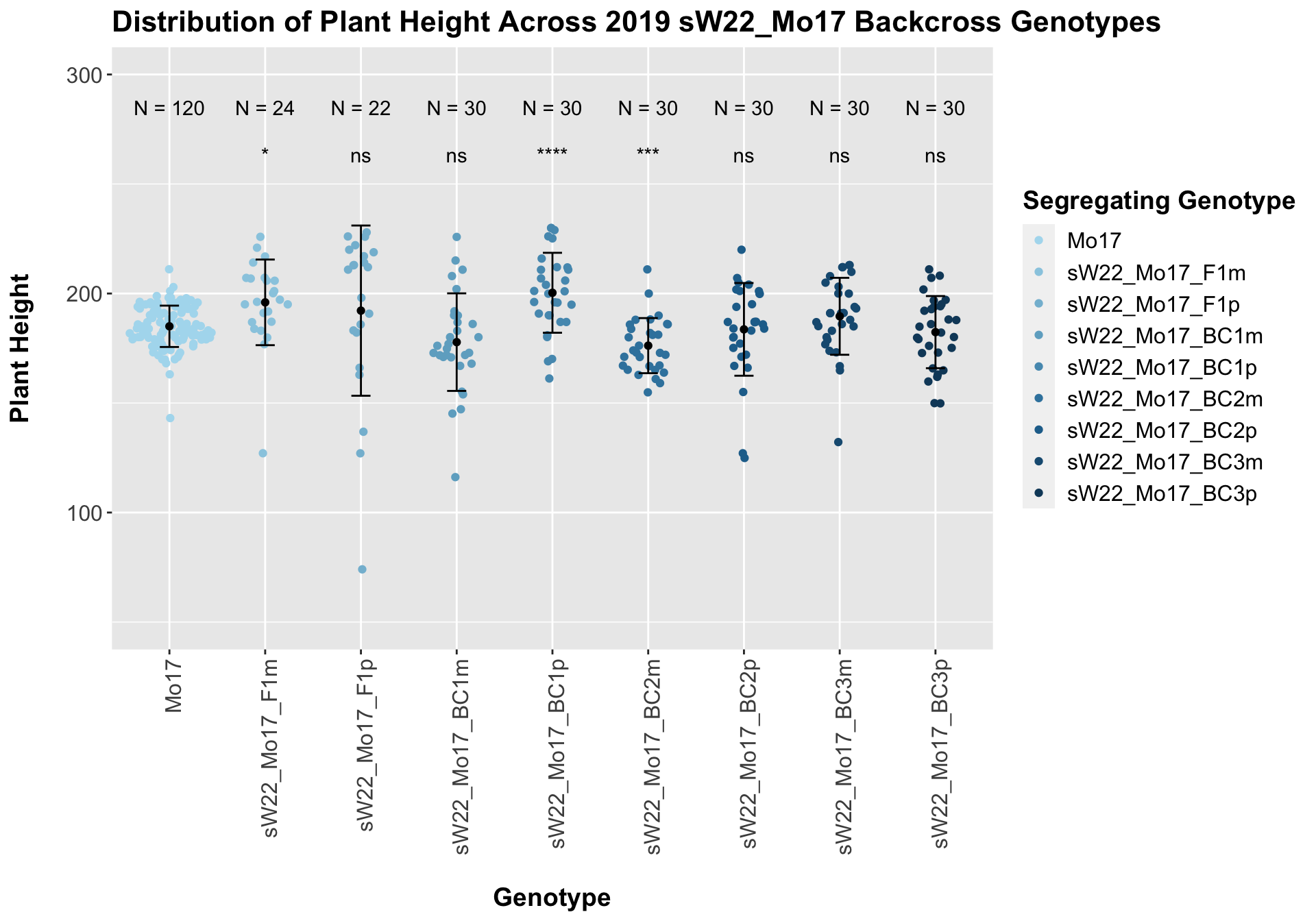
## # A tibble: 8 x 8
##   .y.          group1 group2                 p   p.adj p.format p.signif method
##   <chr>        <chr>  <chr>              <dbl>   <dbl> <chr>    <chr>    <chr>
## 1 Plant_Height Mo17   sW22_Mo17_F1m  0.0129    0.077   0.01285  *        T-test
## 2 Plant_Height Mo17   sW22_Mo17_F1p  0.400     1       0.39977  ns       T-test
## 3 Plant_Height Mo17   sW22_Mo17_BC1m 0.0919    0.46    0.09194  ns       T-test
## 4 Plant_Height Mo17   sW22_Mo17_BC1p 0.0000932 0.00075 9.3e-05  ****     T-test
## 5 Plant_Height Mo17   sW22_Mo17_BC2m 0.000924  0.0065  0.00092  ***      T-test
## 6 Plant_Height Mo17   sW22_Mo17_BC2p 0.728     1       0.72758  ns       T-test
## 7 Plant_Height Mo17   sW22_Mo17_BC3m 0.178     0.71    0.17752  ns       T-test
## 8 Plant_Height Mo17   sW22_Mo17_BC3p 0.401     1       0.40134  ns       T-test
Once again, we find that there is little change in plant height among the F1s and early backcrosses compared to Mo17, but plant height does seem to decline across subsequent backcrosses.
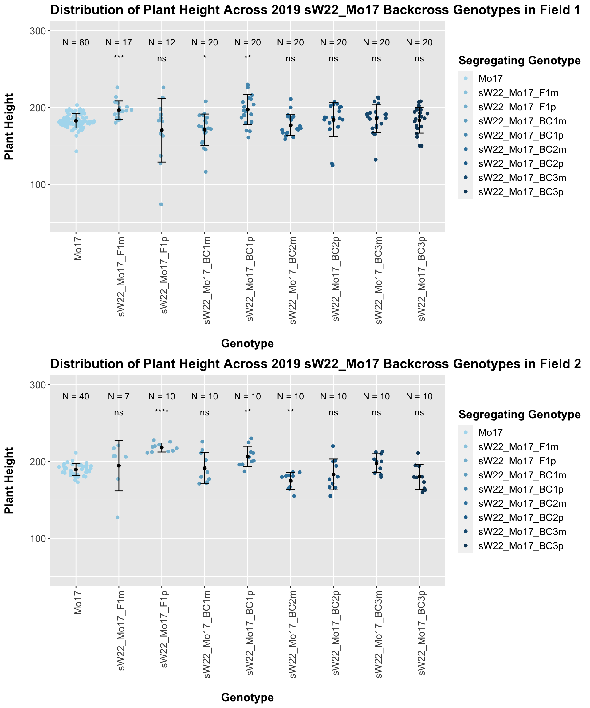
The field data is very similar to the data in aggregate. We can compare the height data across the W22 backcrossed to Mo17 rows.
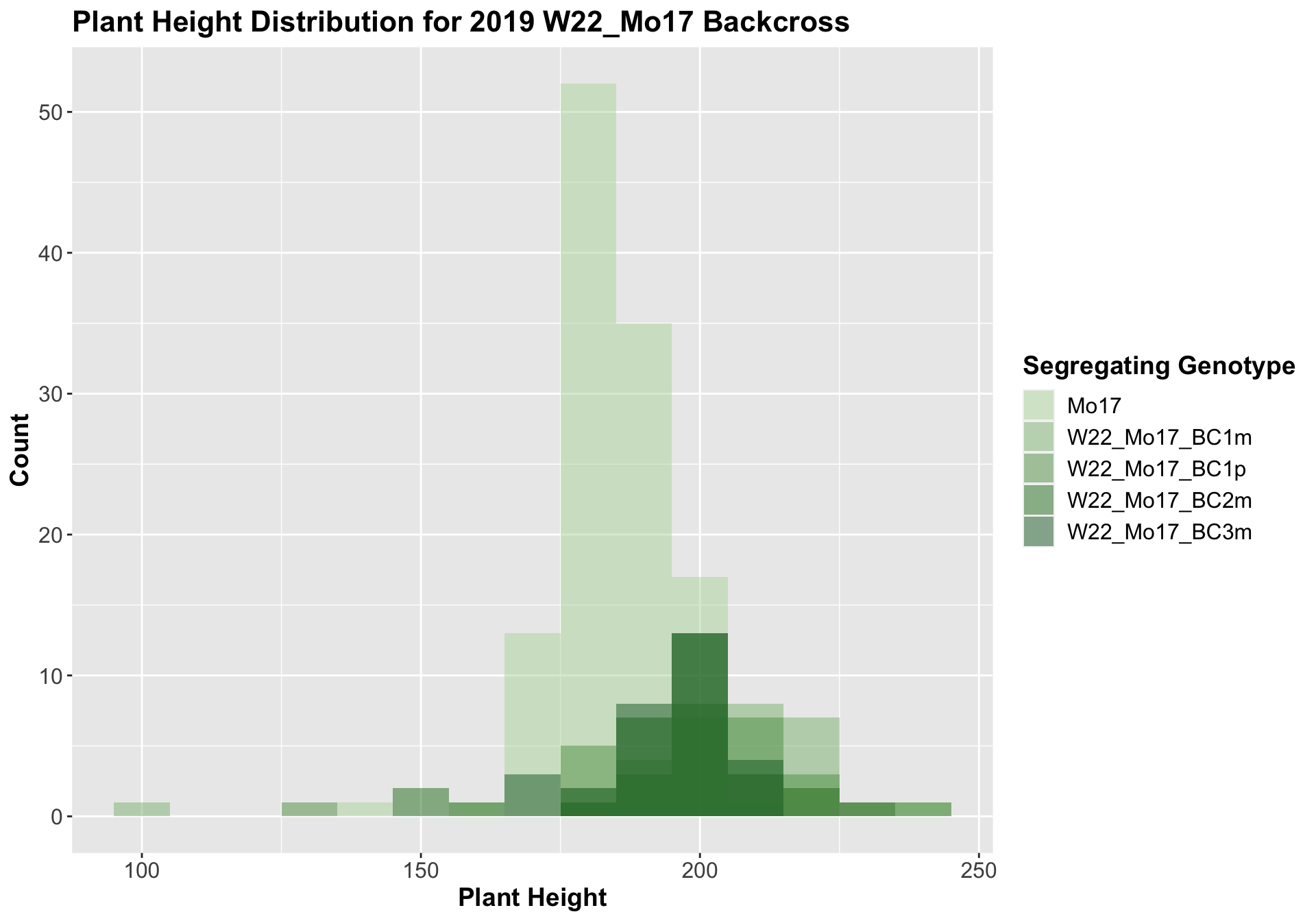
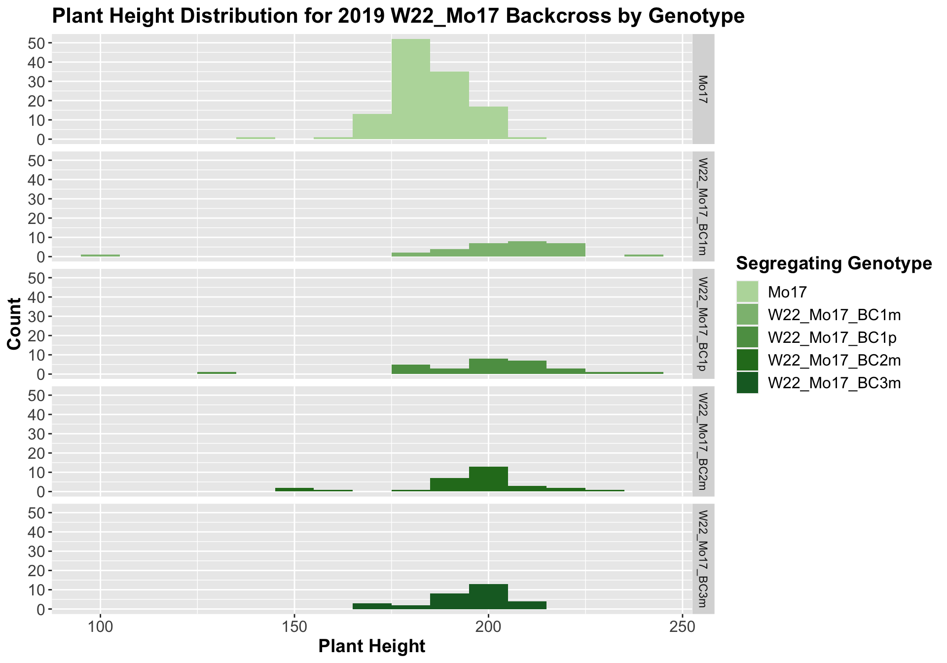
##
##  Mean, SD, and SE for each genotype
## Seg_Genotype N mean sd se
## 1 Mo17 120 185.0250 9.441961 0.8619292
## 2 W22_Mo17_BC1m 30 203.2333 23.890098 4.3617152
## 3 W22_Mo17_BC1p 29 200.7931 20.375720 3.7836761
## 4 W22_Mo17_BC2m 30 196.6000 16.785873 3.0646670
## 5 W22_Mo17_BC3m 30 195.3667 11.232598 2.0507825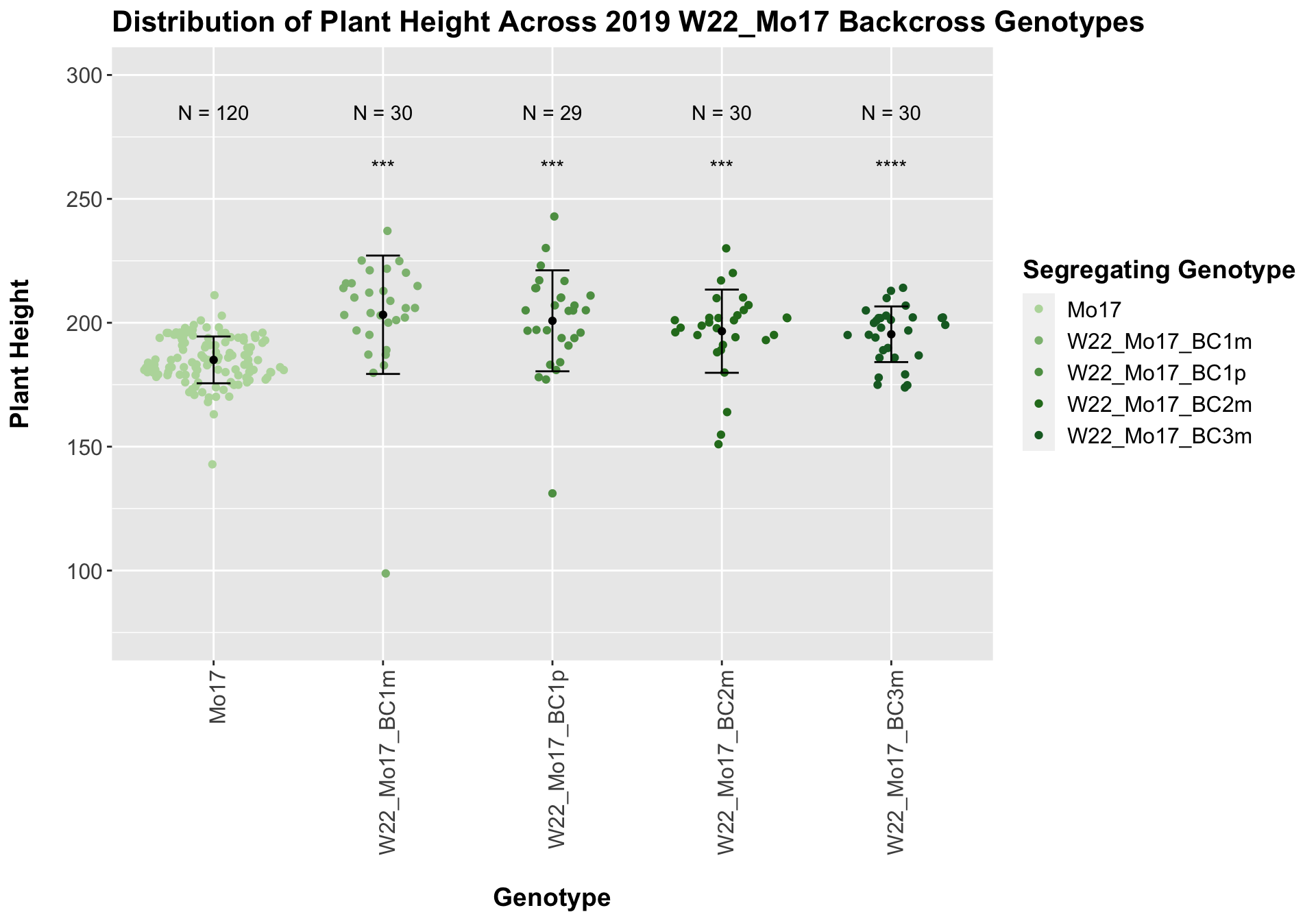
## # A tibble: 4 x 8
##   .y.          group1 group2                p    p.adj p.format p.signif method
##   <chr>        <chr>  <chr>             <dbl>    <dbl> <chr>    <chr>    <chr>
## 1 Plant_Height Mo17   W22_Mo17_BC1m 0.000276  0.00083  0.00028  ***      T-test
## 2 Plant_Height Mo17   W22_Mo17_BC1p 0.000307  0.00083  0.00031  ***      T-test
## 3 Plant_Height Mo17   W22_Mo17_BC2m 0.000914  0.00091  0.00091  ***      T-test
## 4 Plant_Height Mo17   W22_Mo17_BC3m 0.0000362 0.000140 3.6e-05  ****     T-test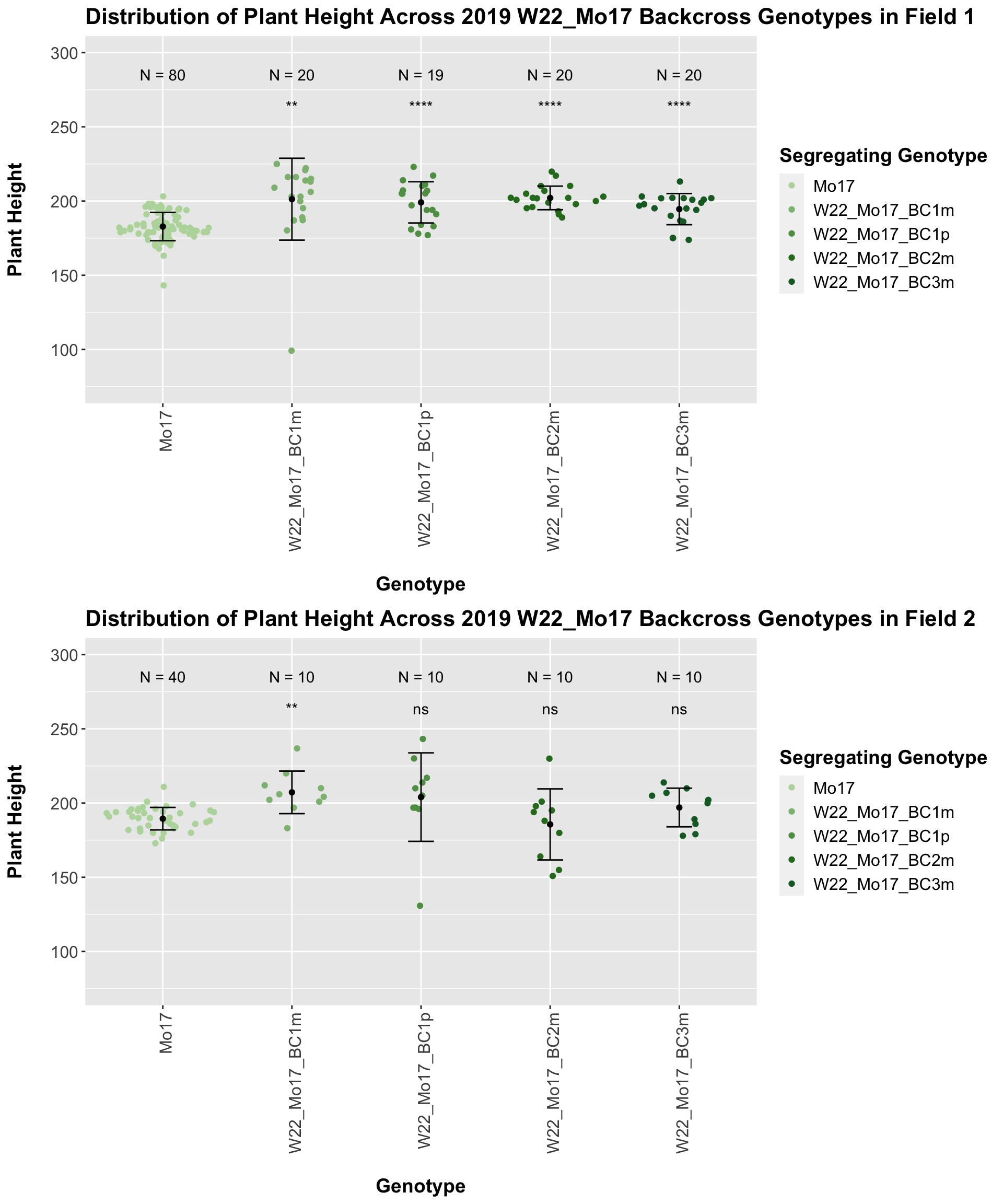
For the W22_Mo17 cross, we once again see an increase in height among early generations followed by a decline. In Field 2, we find that the later generations are not significantly different from the Mo17 line.
We now compare the distribution for sW22_Mo17 backcrosses to W22_Mo17 backcrosses and how each generaiton compares across these two sets. Note: when looking at these plots, just be aware that the genotypes don't align perfectly across backcrosses because we don't have a few crosses for the W22_Mo17 genotypes.
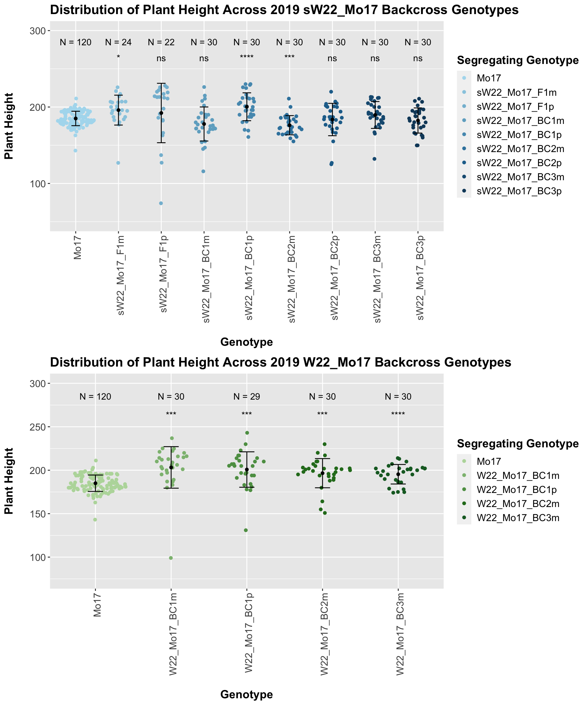
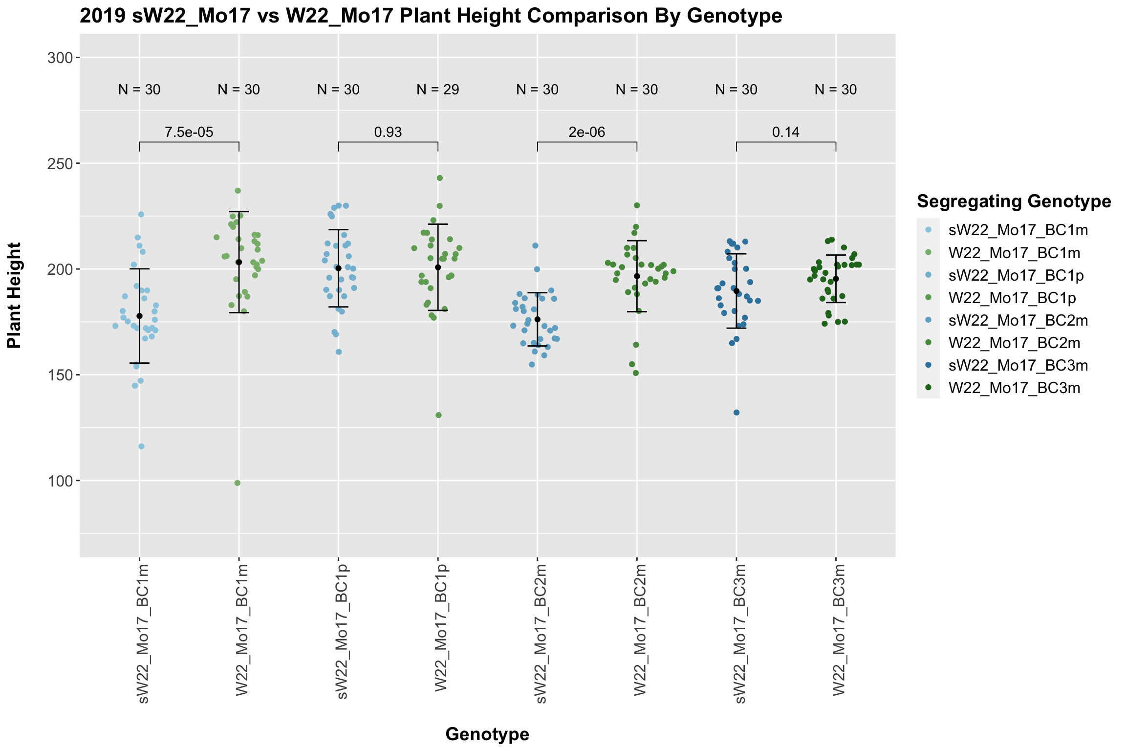
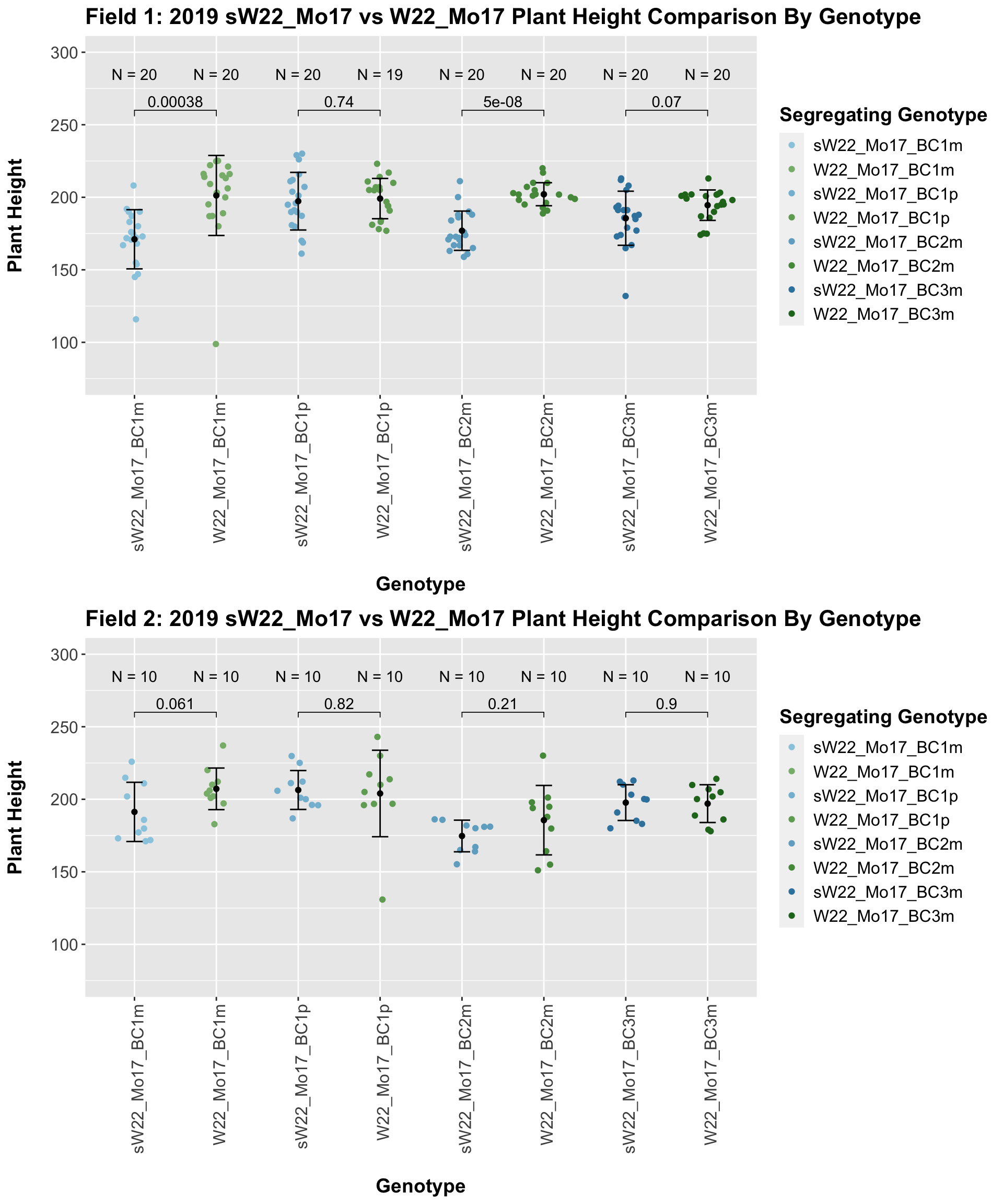
In 2019, we do not see a consistent difference between the sW22_Mo17 and w22_Mo17 backcrosses. 2 of our 4 comparisons show no difference, and this holds even when we stratify the data by field.
We may also be interested the distribution for all sW22 backcrosses (crossed to W22, B73, and Mo17 respectively). Note: when looking at these plots, just be aware that the genotypes don't align perfectly across backcrosses so be sure to check the x-axis.
3.1.4 2019 ANOVA for Plant Height
So far, we have only tested the difference of each segregating genotype against the external control it has been backcrossed to. We now want to test whether (1) ear height is impacted by the sex of the sick parent and (2) the means across each backcross generation change NOTE: I was not fully confident in how/whether to incorporate the external stock information (W22, B73,Mo17) as these lineages were selfed and therefore had no sick parent to test the sex of. We also transformed the categorical genotype values (F1,BC1,BC2,BC3,BC4,BC5) to numerical values (0,1,2,3,4,5). NOTE: I'm not sure if this is appropriate. It'd be fairly simple to switch this back to categorical values if that would be better
We start by fitting a series of linear models:
- mod_full_int: Plant_Height (Numerical) ~ Field (Cateogrical) + Genotype (Numerical) + Sick_Sex (Categorical) + Genotype*Sick_Sex
- mod_full: Plant_Height (Numerical) ~ Field (Categorical) + Genotype (Numerical) + Sick_Sex (Categorical)
- mod_geno: Plant_Height (Numerical) ~ Field (Cateogrical) + Genotype (Numerical)
- mod_sex: Plant_Height (Numerical) ~ Field + Sick_Sex (Categorical)
We can then compare the fit of these models to our data using an ANOVA to test whether the more complex model (mod_full) is significantly better at capturing our height data than either of our simpler models. This will tell us whether incorporating sex/genotype significantly improves our model.
We can summarize the results of this across each set of genotypes. The significance codes are as follows:
- '***' - between 0 and 0.001
- '**' - between 0.001 and 0.01
- '*' - between 0.01 and 0.05
- '.' - between 0.05 and 0.1
- ' ' - between 0.1 and 1
##    Geno_Set   Sex_PValue Sex_Signif Genotype_PValue Genotype_Signif
## 1  sW22_W22 3.162755e-08        ***    6.130627e-01
## 2  sW22_B73 9.182240e-02          .    5.865215e-07             ***
## 3 sW22_Mo17 9.085188e-02          .    1.915423e-02               *
## 4   W22_B73 2.220765e-02          *    1.776534e-04             ***
## 5  W22_Mo17 7.432257e-01               1.056457e-01
##   Sex_Geno_Int_PValue Sex_Geno_Int_Signif
## 1           0.4250684
## 2           0.6596666
## 3           0.2426715
## 4           0.2830893
## 5                  NA
For 2019, we do not find that genotype is consistently a significant term, and we do not find that there is ever a significant interaction between sex and genotype.
3.2 2020 Plant Height Data
3.2.1 2020 sW22 backcrossed to W22
##
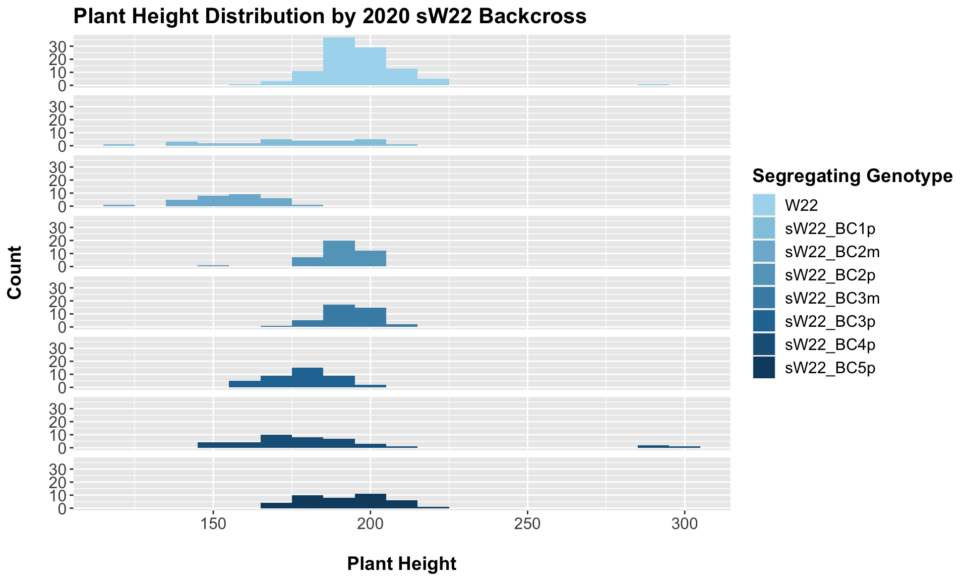
## Mean, SD, and SE for each genotype## Seg_Genotype N mean sd se
## 1 W22 100 196.6000 14.854853 1.485485
## 2 sW22_BC1p 27 175.4444 23.008917 4.428068
## 3 sW22_BC2m 30 155.1000 13.376124 2.442135
## 4 sW22_BC2p 40 191.1000 9.158994 1.448164
## 5 sW22_BC3m 40 194.1250 7.473672 1.181691
## 6 sW22_BC3p 40 179.2750 10.585398 1.673698
## 7 sW22_BC4p 40 185.1250 34.393043 5.438018
## 8 sW22_BC5p 40 192.4750 12.778161 2.020405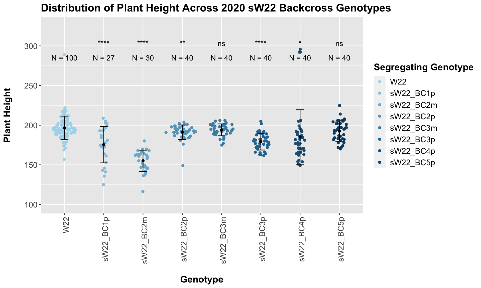
##
## Results of T-test used to obtain significance in the above plot
## # A tibble: 7 x 8
## .y. group1 group2 p p.adj p.format p.signif method
## <chr> <chr> <chr> <dbl> <dbl> <chr> <chr> <chr>
## 1 Plant_Height W22 sW22_BC1p 7.72e- 5 3.90e- 4 7.7e-05 **** T-test
## 2 Plant_Height W22 sW22_BC2m 5.43e-20 3.80e-19 < 2e-16 **** T-test
## 3 Plant_Height W22 sW22_BC2p 9.16e- 3 3.70e- 2 0.0092 ** T-test
## 4 Plant_Height W22 sW22_BC3m 1.95e- 1 2.10e- 1 0.1946 ns T-test
## 5 Plant_Height W22 sW22_BC3p 8.06e-12 4.80e-11 8.1e-12 **** T-test
## 6 Plant_Height W22 sW22_BC4p 4.77e- 2 1.40e- 1 0.0477 * T-test
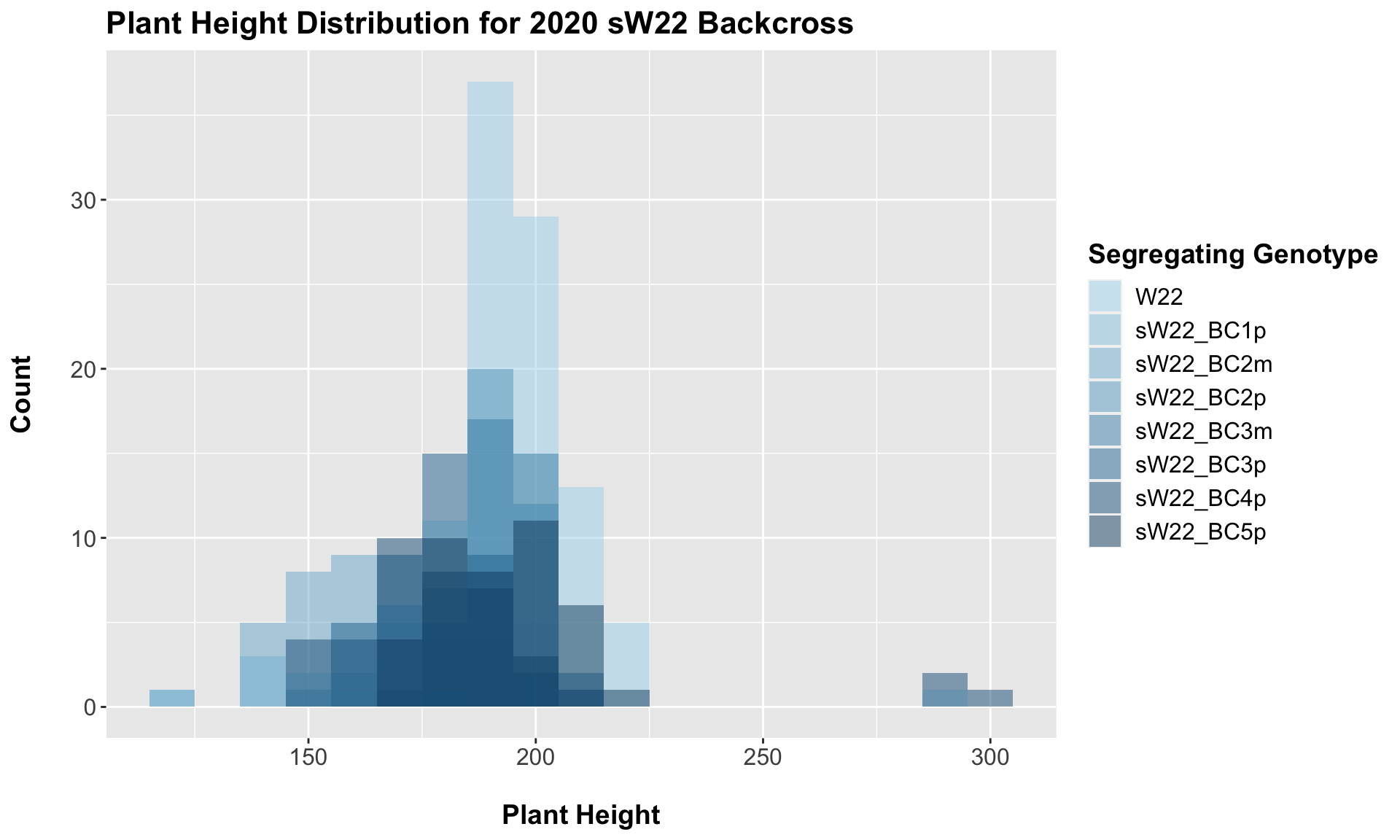
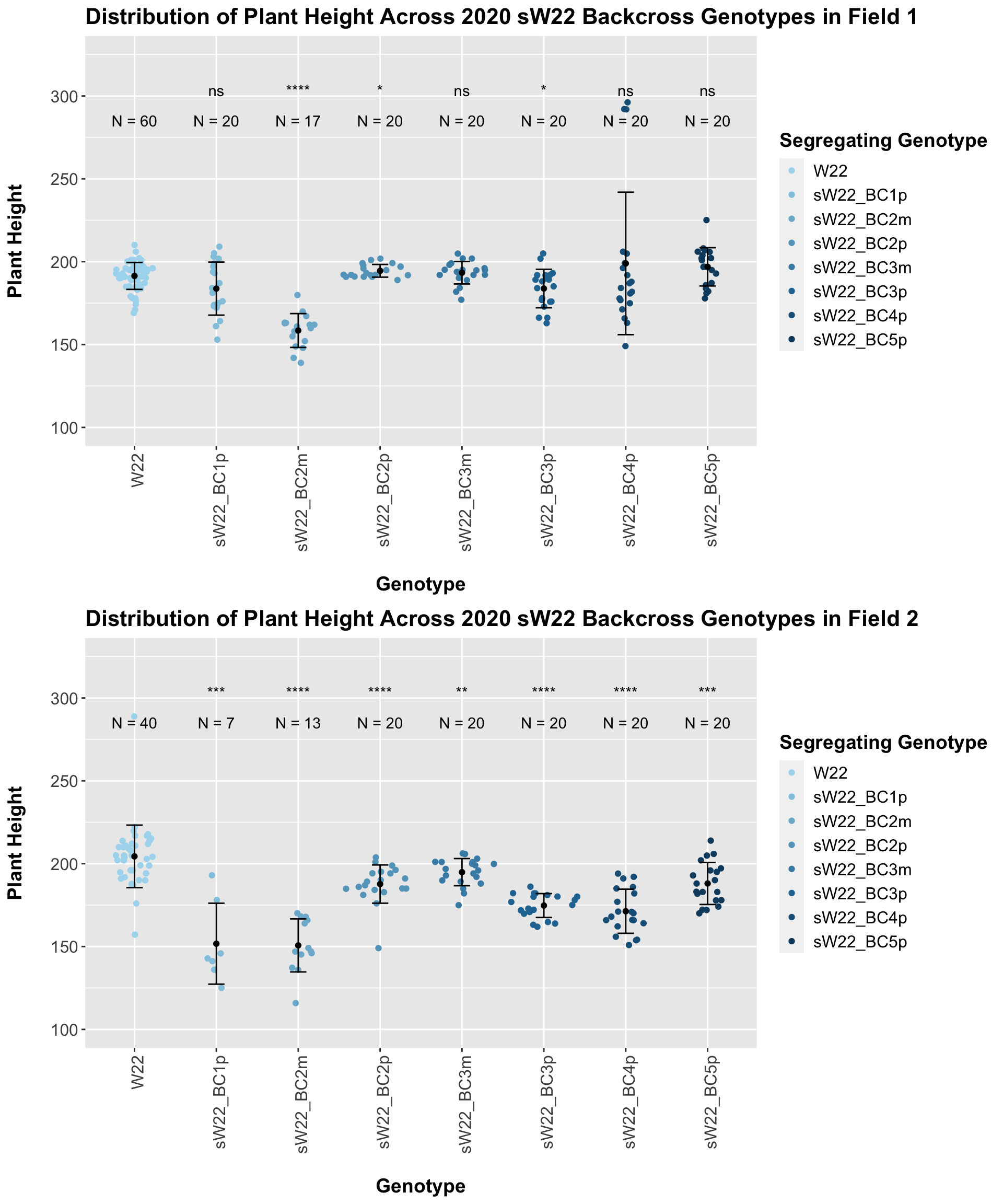
## 7 Plant_Height W22 sW22_BC5p 1.04e- 1 2.10e- 1 0.1038 ns T-testFor our sW22 backcrossed to W22, we see a similar trend to that in 2019. There is an initial reduction in plant height that increases after each generation of backcrossing. We can once again check that this trend holds if we stratify the data by field.
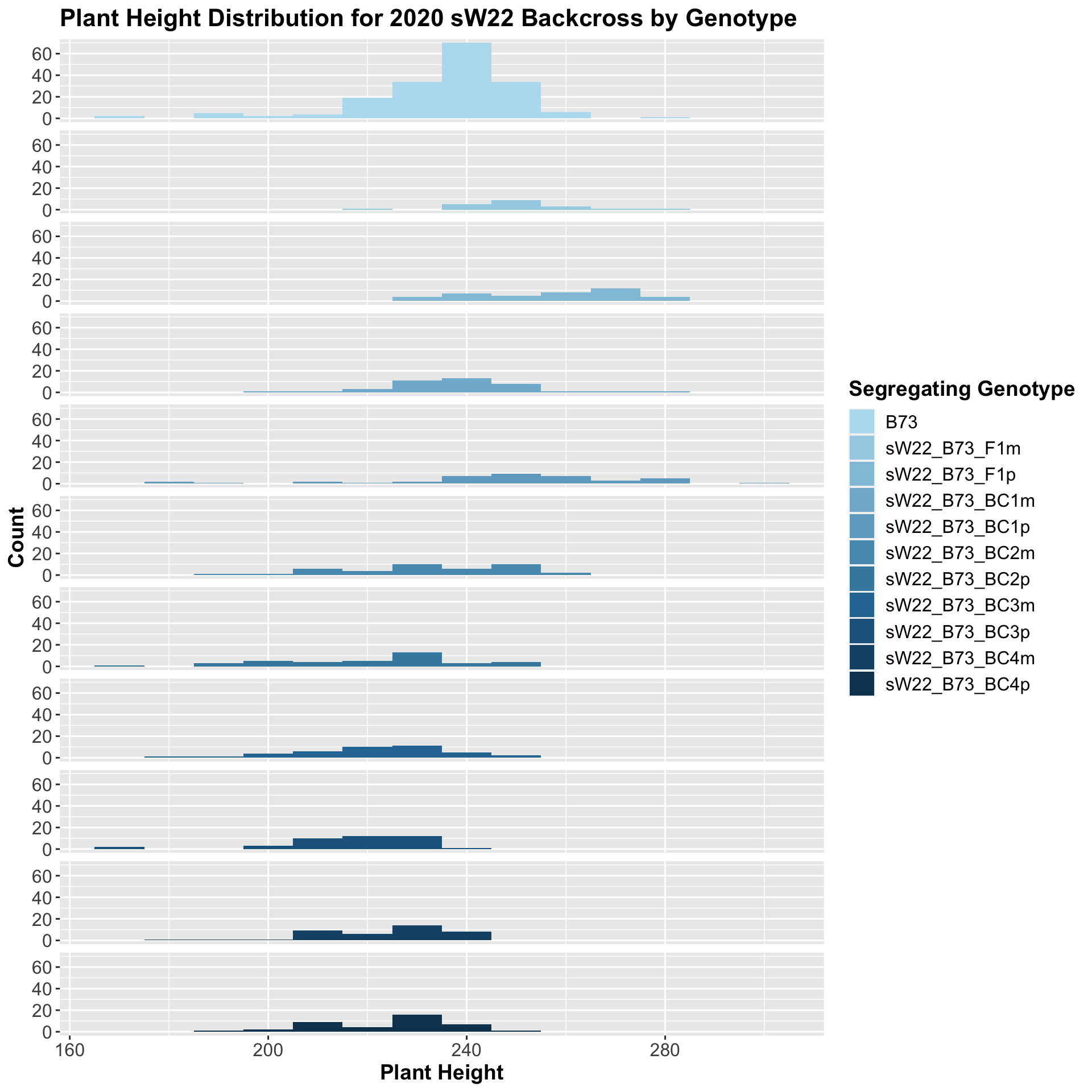
3.2.2 2020 sW22 and W22 backcrossed to B73
##
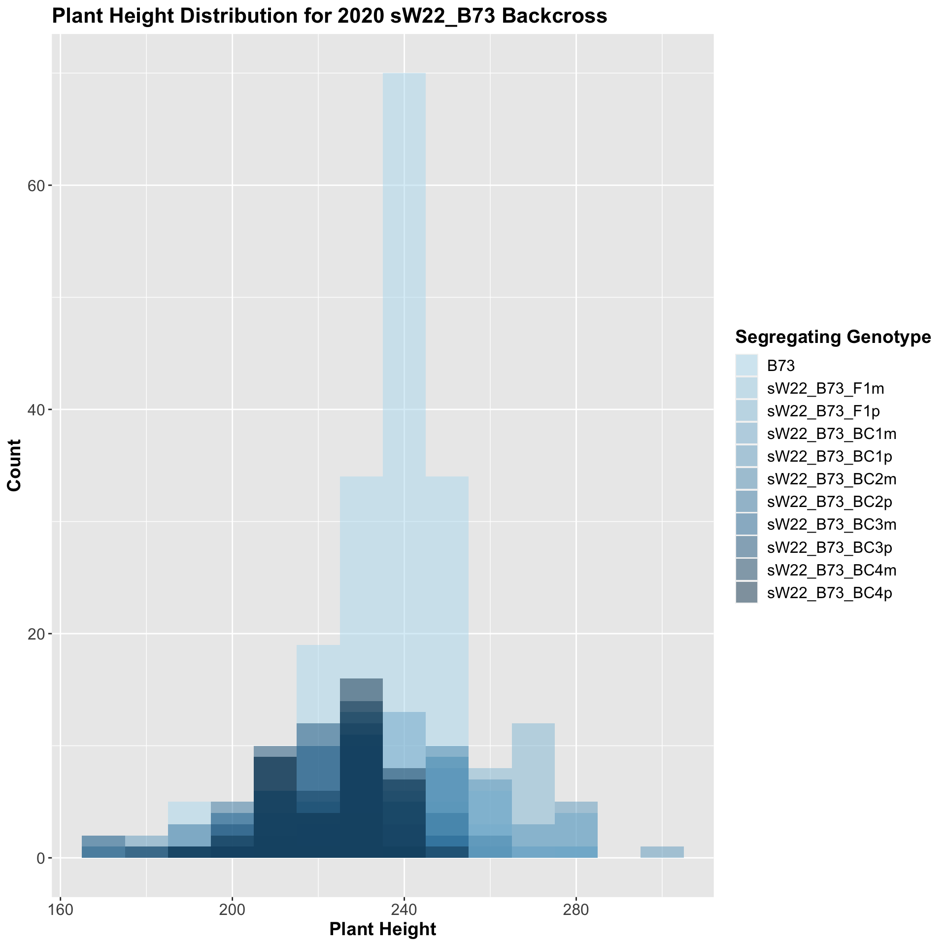
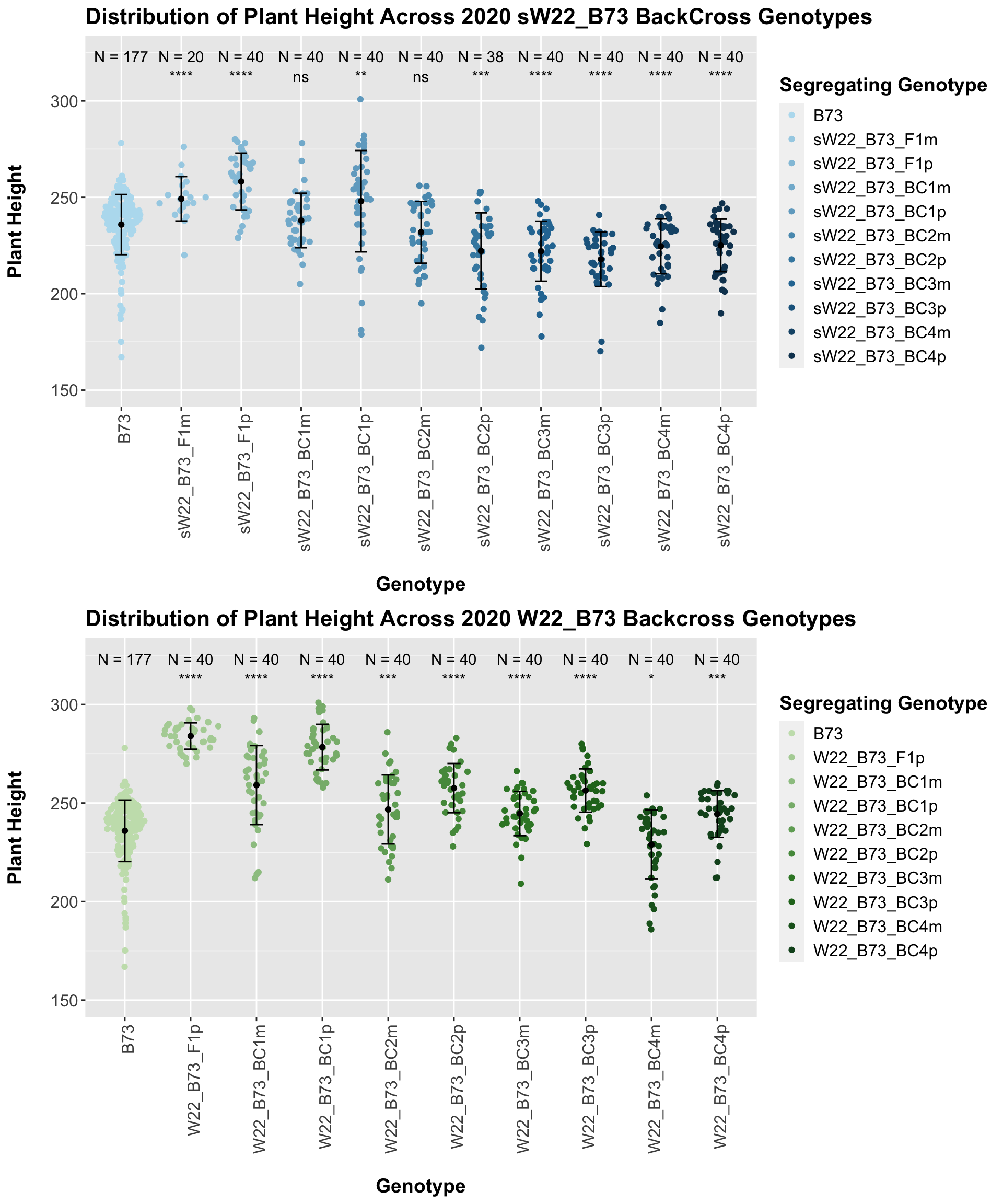
## Mean, SD, and SE for each genotype## Seg_Genotype N mean sd se
## 1 B73 177 235.8870 15.61063 1.173367
## 2 sW22_B73_F1m 20 249.2500 11.50686 2.573013
## 3 sW22_B73_F1p 40 258.2250 14.73612 2.329985
## 4 sW22_B73_BC1m 40 238.0000 14.15120 2.237501
## 5 sW22_B73_BC1p 40 248.0000 26.30394 4.159019
## 6 sW22_B73_BC2m 40 231.8750 16.02592 2.533921
## 7 sW22_B73_BC2p 38 222.1842 19.76190 3.205804
## 8 sW22_B73_BC3m 40 222.0750 15.57675 2.462901
## 9 sW22_B73_BC3p 40 217.8750 14.12252 2.232966
## 10 sW22_B73_BC4m 40 224.5750 14.20705 2.246332
## 11 sW22_B73_BC4p 40 225.0500 13.62304 2.153992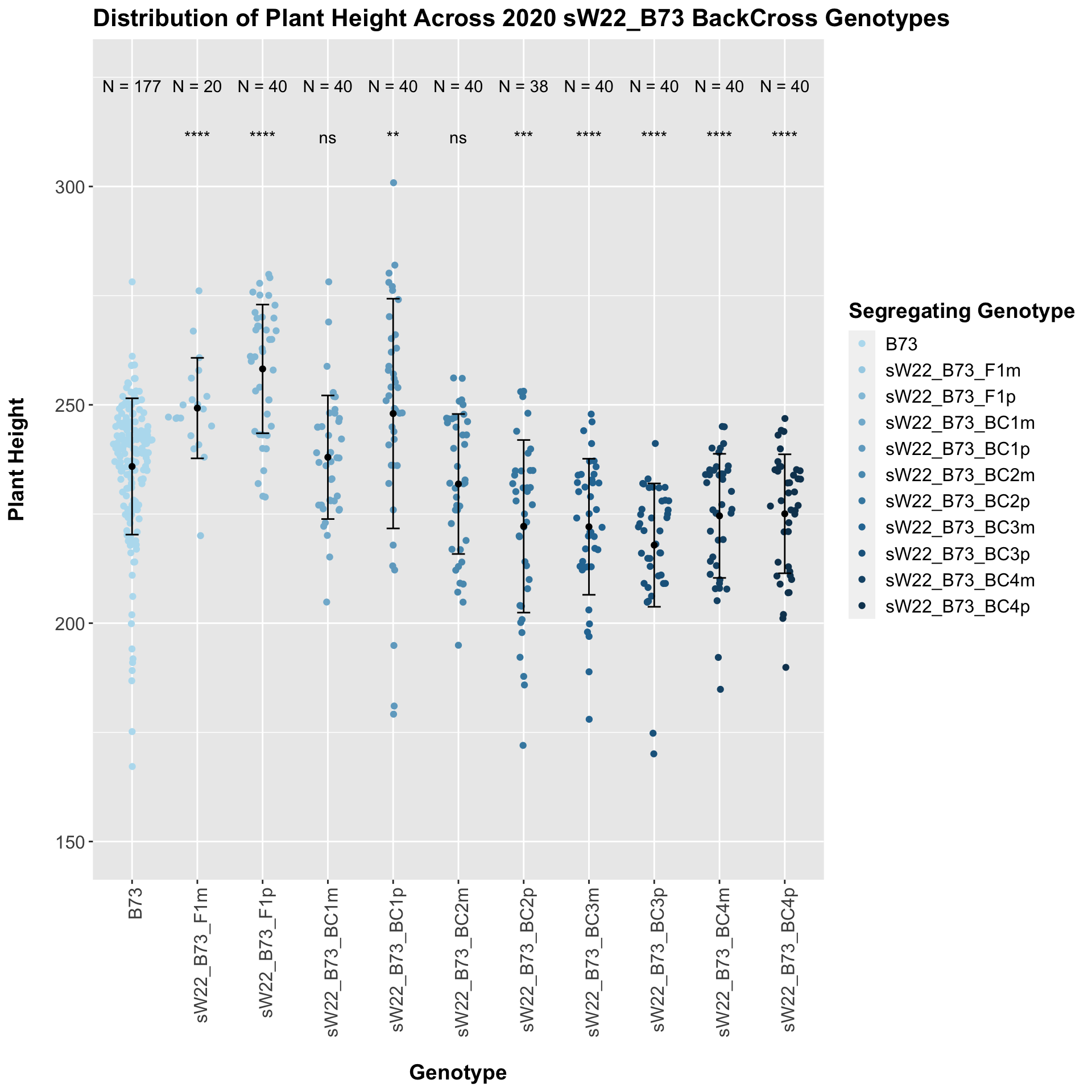
## # A tibble: 10 x 8
##    .y.          group1 group2               p    p.adj p.format p.signif method
##    <chr>        <chr>  <chr>            <dbl>    <dbl> <chr>    <chr>    <chr>
##  1 Plant_Height B73    sW22_B73_F1m  6.07e- 5 3.00e- 4 6.1e-05  ****     T-test
##  2 Plant_Height B73    sW22_B73_F1p  5.12e-12 5.10e-11 5.1e-12  ****     T-test
##  3 Plant_Height B73    sW22_B73_BC1m 4.06e- 1 4.10e- 1 0.40616  ns       T-test
##  4 Plant_Height B73    sW22_B73_BC1p 7.42e- 3 2.20e- 2 0.00742  **       T-test
##  5 Plant_Height B73    sW22_B73_BC2m 1.56e- 1 3.10e- 1 0.15626  ns       T-test
##  6 Plant_Height B73    sW22_B73_BC2p 2.11e- 4 8.50e- 4 0.00021  ***      T-test
##  7 Plant_Height B73    sW22_B73_BC3m 4.47e- 6 3.60e- 5 4.5e-06  ****     T-test
##  8 Plant_Height B73    sW22_B73_BC3p 1.18e- 9 1.10e- 8 1.2e-09  ****     T-test
##  9 Plant_Height B73    sW22_B73_BC4m 3.46e- 5 2.40e- 4 3.5e-05  ****     T-test
## 10 Plant_Height B73    sW22_B73_BC4p 3.90e- 5 2.40e- 4 3.9e-05  ****     T-test
We see an initial increase in plant height among the F1s that slowly decrease after each generation of backcrossing to B73. We can check whether or not this trend holds if we stratify by field.
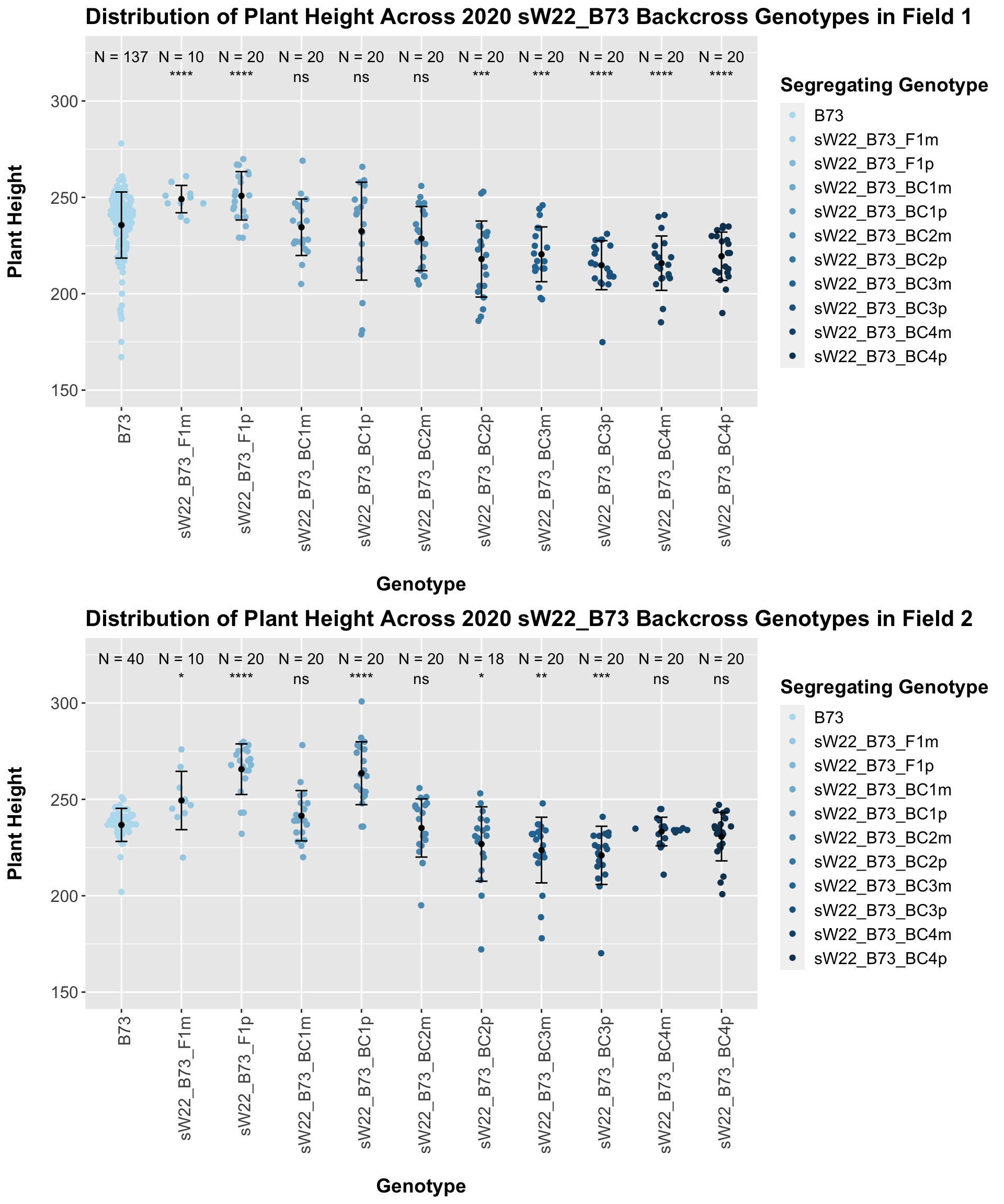
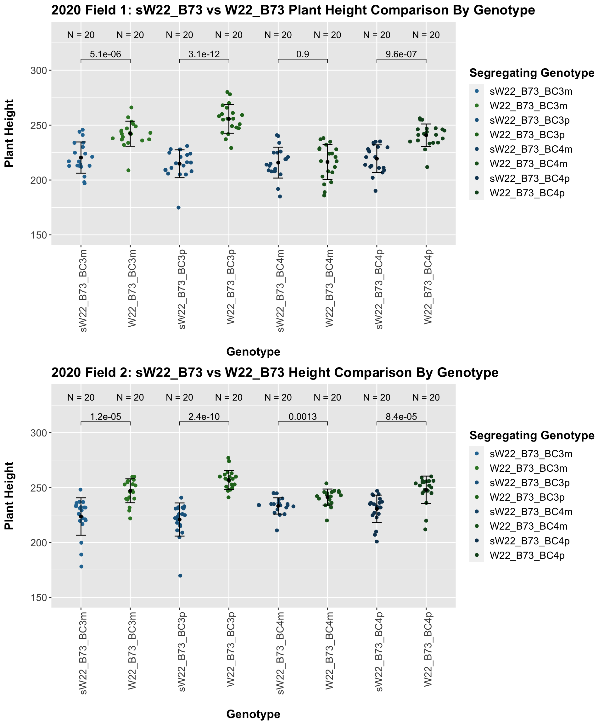
It seems as if though the trend holds after stratifying by field, but there is a bit more variation in plant heigh seen in Field 2.
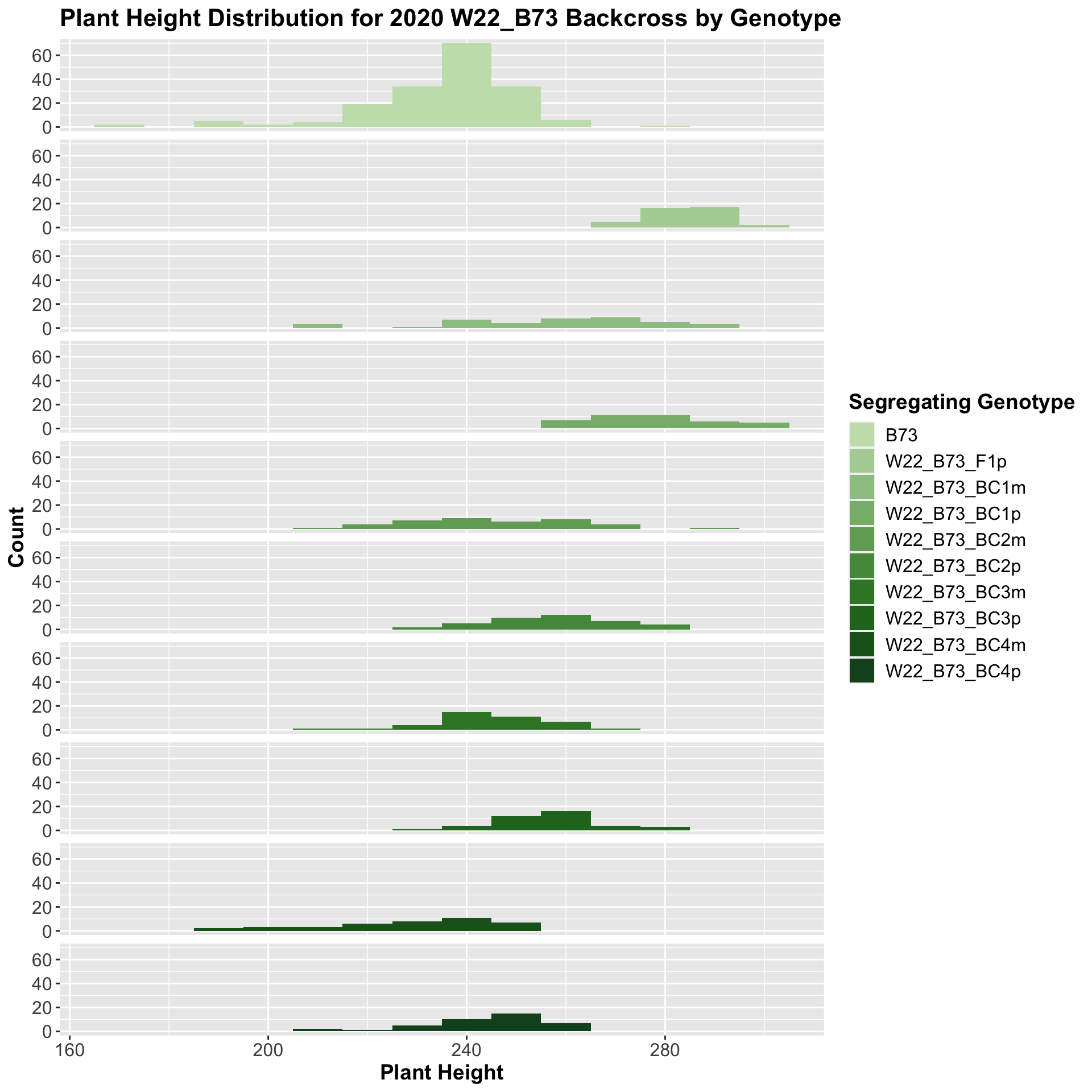
We also want to look at the height data across the W22 backcrossed to B73 rows.
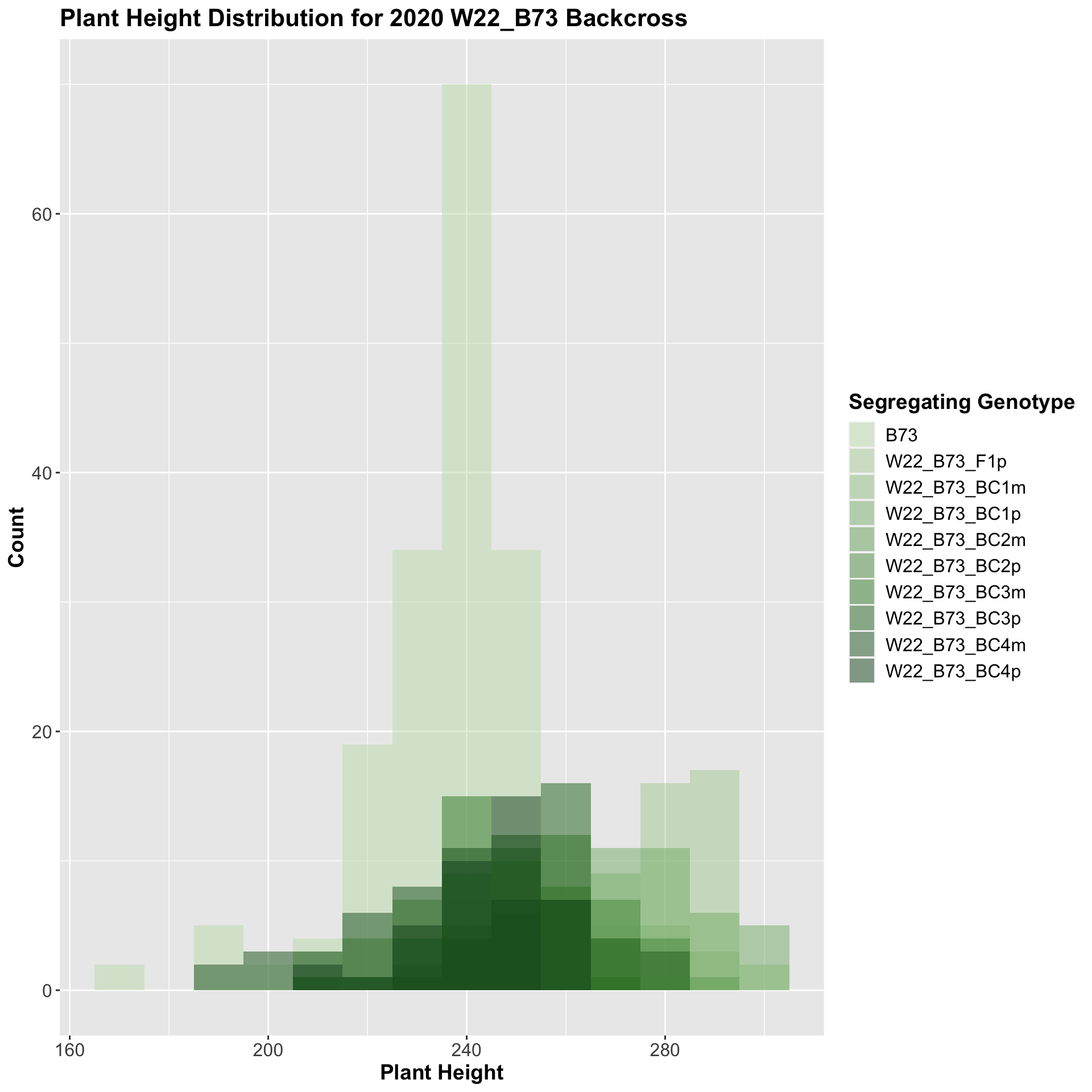
##
##  Mean, SD, and SE for each genotype
## Seg_Genotype N mean sd se
## 1 B73 177 235.887 15.610628 1.173367
## 2 W22_B73_F1p 40 283.975 6.689017 1.057626
## 3 W22_B73_BC1m 40 259.075 20.046596 3.169645
## 4 W22_B73_BC1p 40 278.350 11.588124 1.832243
## 5 W22_B73_BC2m 40 246.725 17.514811 2.769335
## 6 W22_B73_BC2p 40 257.550 12.498102 1.976124
## 7 W22_B73_BC3m 40 244.650 11.267266 1.781511
## 8 W22_B73_BC3p 40 256.325 10.988076 1.737367
## 9 W22_B73_BC4m 40 228.925 17.595727 2.782129
## 10 W22_B73_BC4p 40 244.400 11.846886 1.873157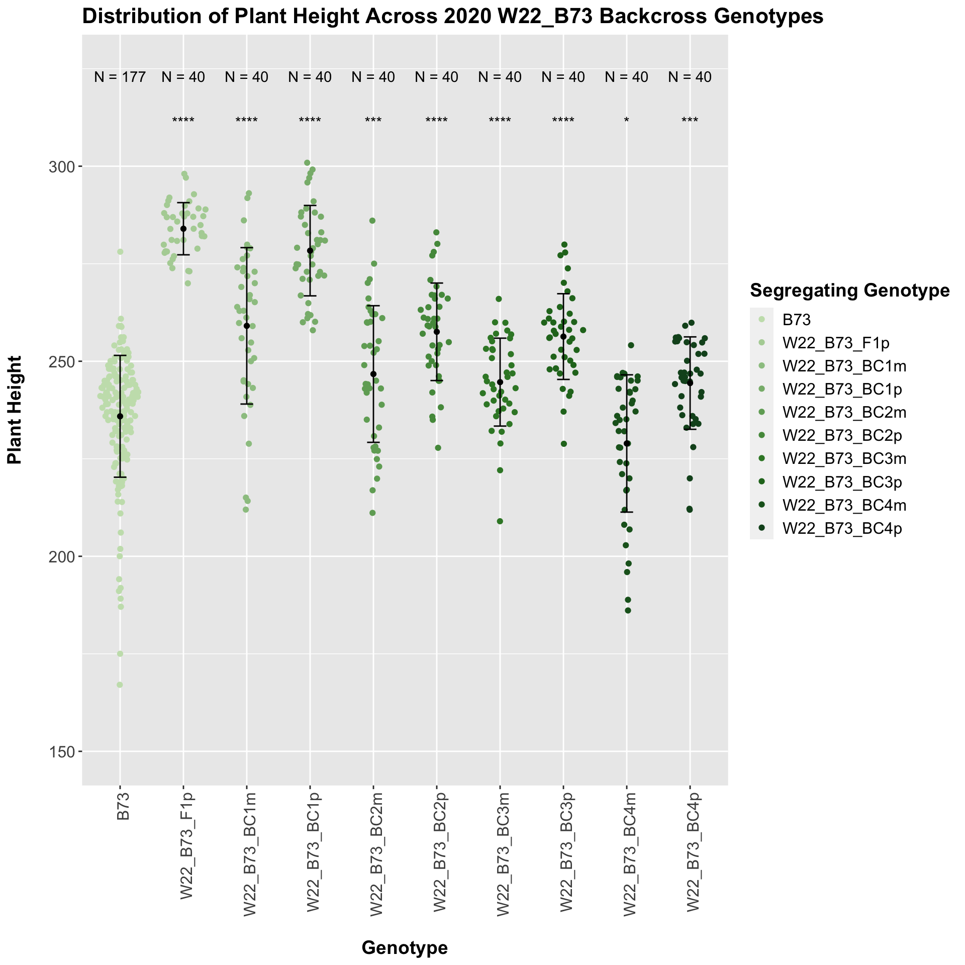
## # A tibble: 9 x 8
##   .y.          group1 group2              p    p.adj p.format p.signif method
##   <chr>        <chr>  <chr>           <dbl>    <dbl> <chr>    <chr>    <chr>
## 1 Plant_Height B73    W22_B73_F1p  6.22e-65 5.60e-64 < 2e-16  ****     T-test
## 2 Plant_Height B73    W22_B73_BC1m 9.72e- 9 4.90e- 8 9.7e-09  ****     T-test
## 3 Plant_Height B73    W22_B73_BC1p 4.56e-31 3.60e-30 < 2e-16  ****     T-test
## 4 Plant_Height B73    W22_B73_BC2m 6.86e- 4 1.40e- 3 0.00069  ***      T-test
## 5 Plant_Height B73    W22_B73_BC2p 4.75e-14 2.80e-13 4.7e-14  ****     T-test
## 6 Plant_Height B73    W22_B73_BC3m 9.88e- 5 4.00e- 4 9.9e-05  ****     T-test
## 7 Plant_Height B73    W22_B73_BC3p 3.37e-15 2.40e-14 3.4e-15  ****     T-test
## 8 Plant_Height B73    W22_B73_BC4m 2.50e- 2 2.50e- 2 0.02501  *        T-test
## 9 Plant_Height B73    W22_B73_BC4p 2.50e- 4 7.50e- 4 0.00025  ***      T-test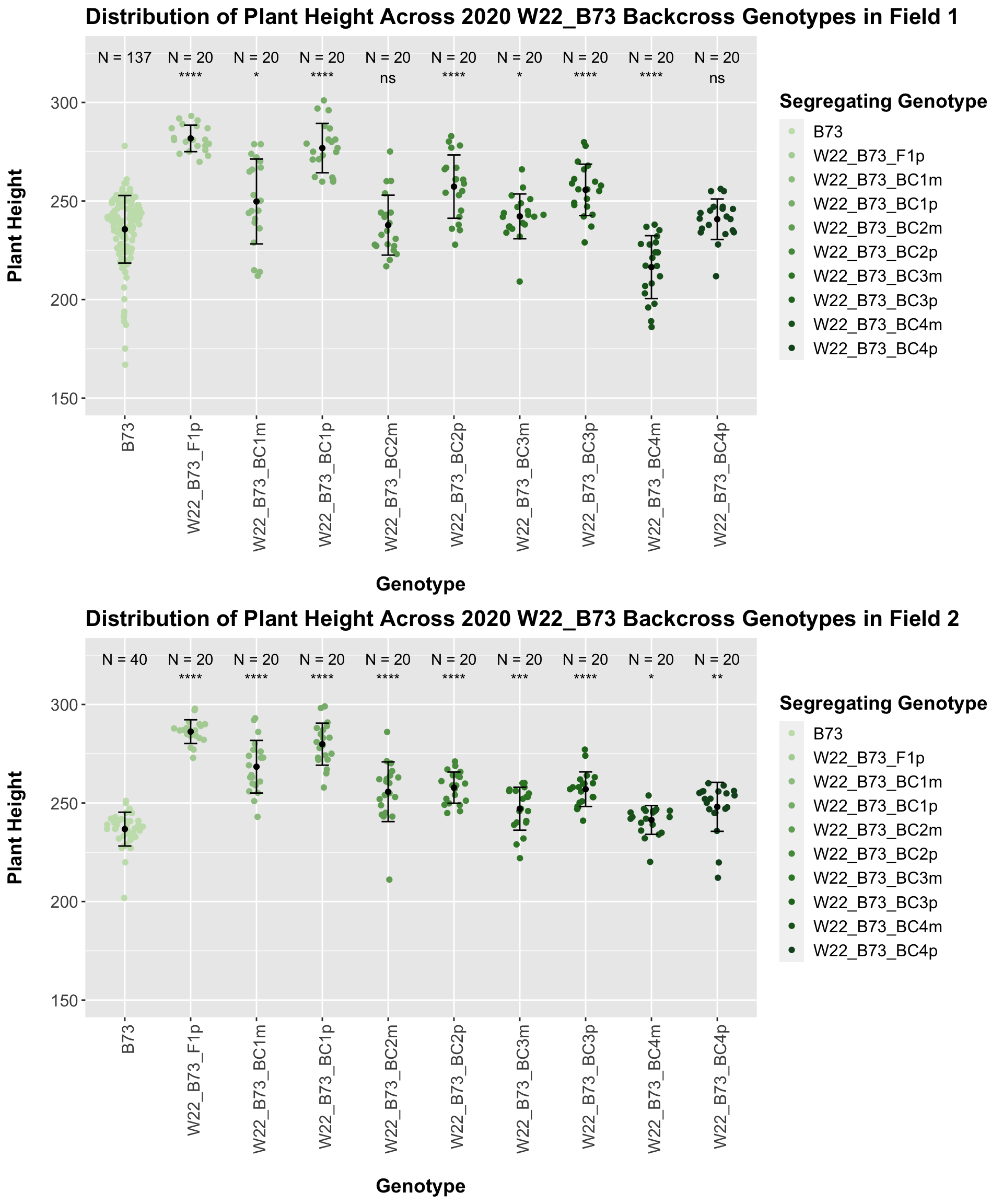
We see a similar trend, where the F1s exhibit an increase in plant height which decreases after each generation of backcrossing. We now want to compare the sW22 backcrosses to the W22 backcrosses at each generation. Note: when looking at these plots, just be aware that the genotypes don't align perfectly across backcrosses because we don't have a few crosses for the W22_B73 genotypes.
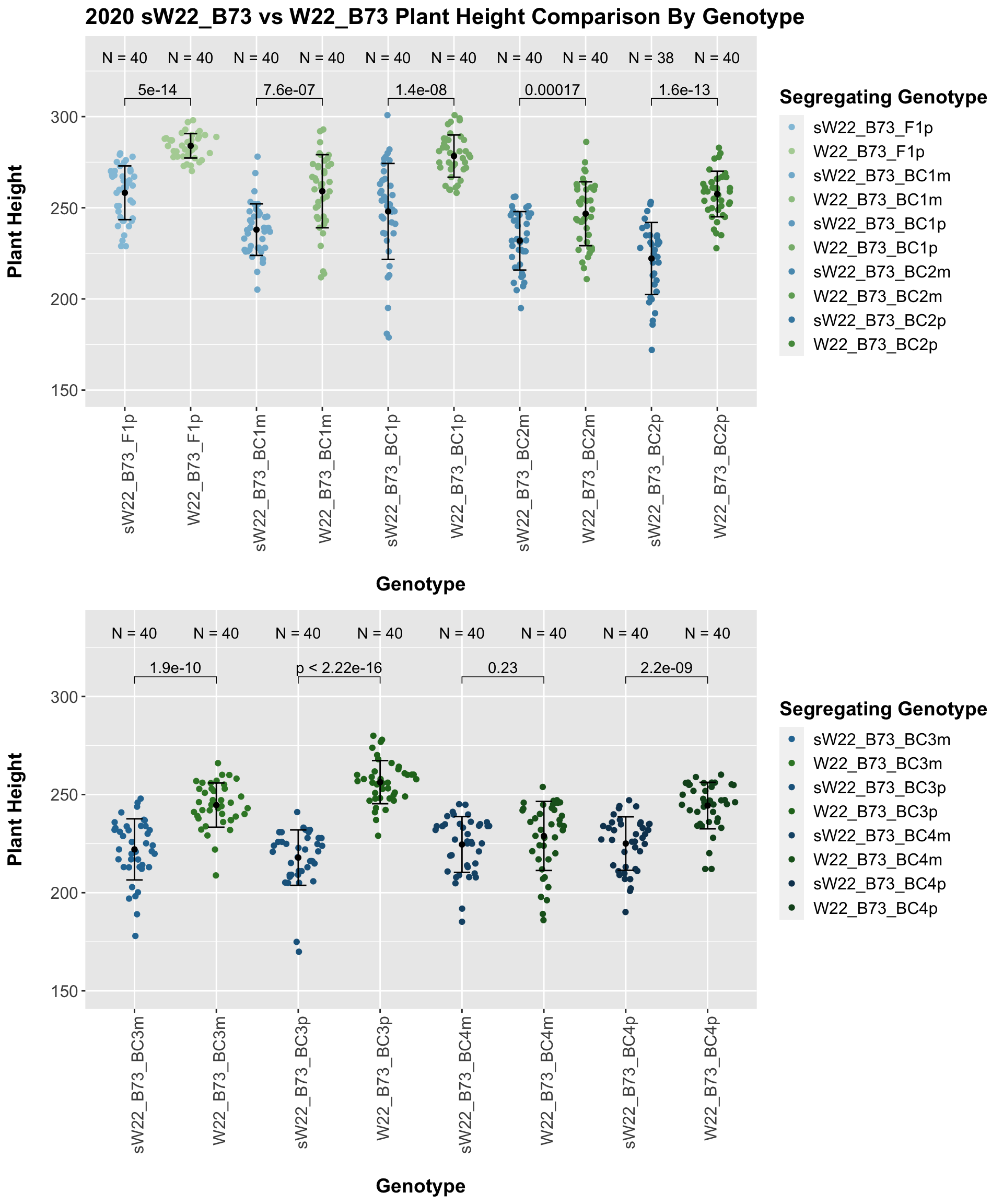
## List of 1
##  $ axis.text.x:List of 11
##   ..$ family       : NULL
##   ..$ face         : NULL
##   ..$ colour       : NULL
##   ..$ size         : NULL
##   ..$ hjust        : num 1
##   ..$ vjust        : num 0.75
##   ..$ angle        : num 90
##   ..$ lineheight   : NULL
##   ..$ margin       : NULL
##   ..$ debug        : NULL
##   ..$ inherit.blank: logi FALSE
##   ..- attr(*, "class")= chr [1:2] "element_text" "element"
##  - attr(*, "class")= chr [1:2] "theme" "gg"
##  - attr(*, "complete")= logi FALSE
##  - attr(*, "validate")= logi TRUE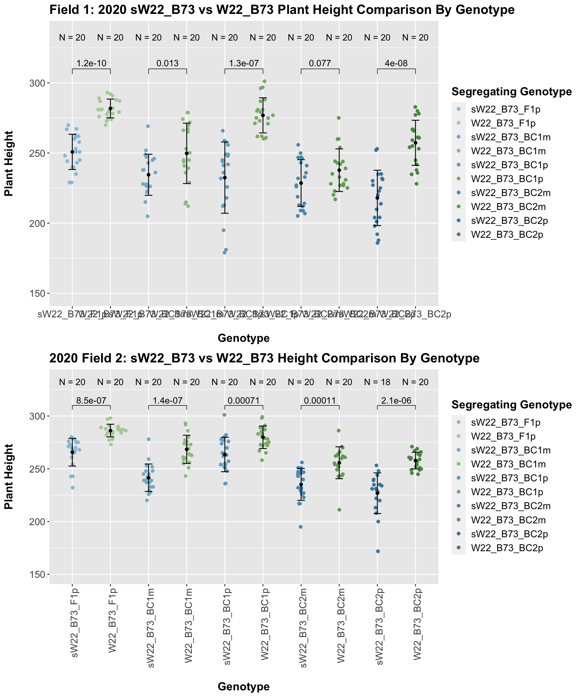
3.2.3 2020 sW22 and W22 backcrossed to Mo17
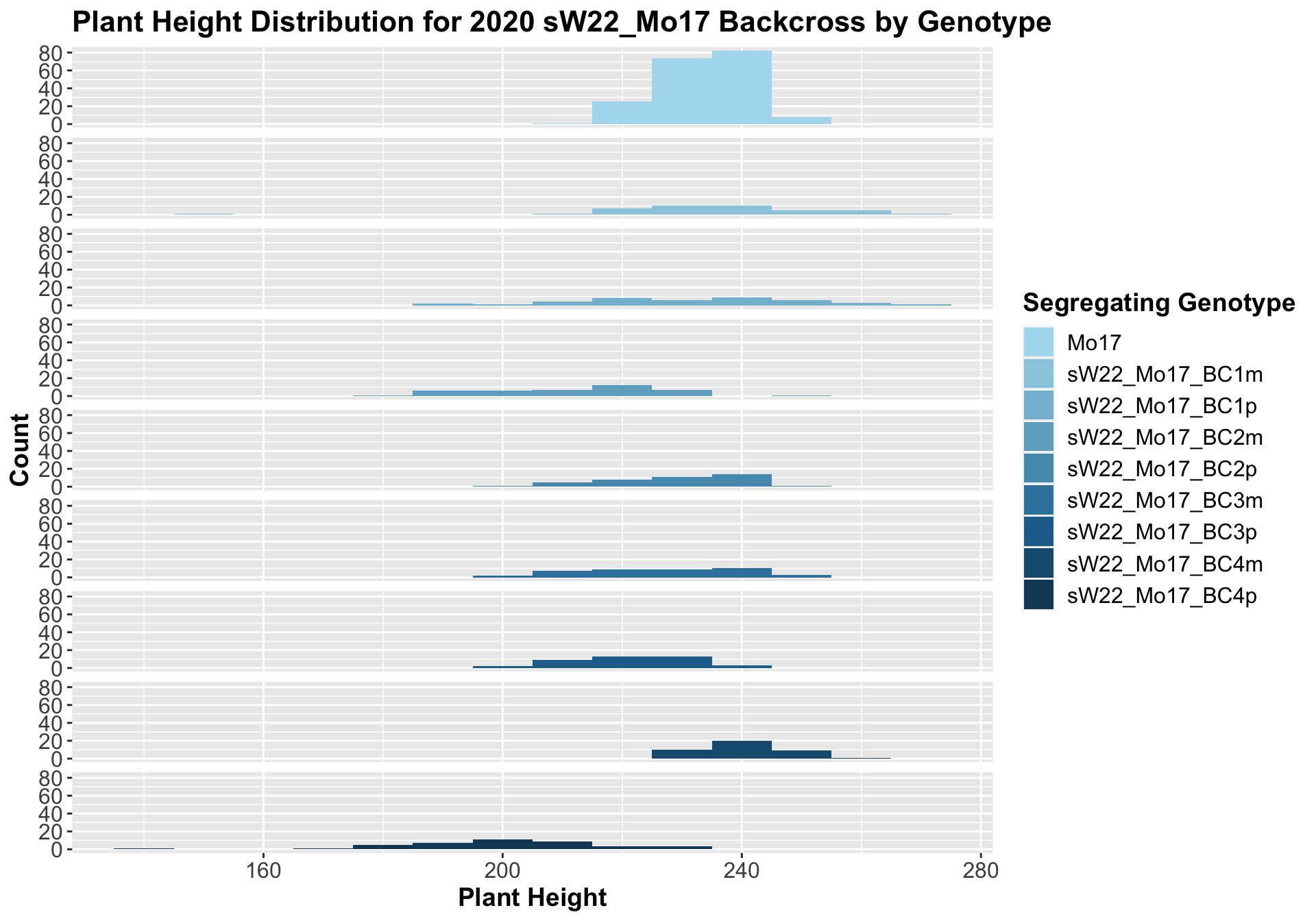
##
##  Mean, SD, and SE for each genotype
## Seg_Genotype N mean sd se
## 1 Mo17 190 233.8316 7.285054 0.5285134
## 2 sW22_Mo17_BC1m 40 235.9250 19.967136 3.1570815
## 3 sW22_Mo17_BC1p 40 232.1500 17.986533 2.8439206
## 4 sW22_Mo17_BC2m 40 213.4500 15.229779 2.4080394
## 5 sW22_Mo17_BC2p 40 229.6500 11.310422 1.7883347
## 6 sW22_Mo17_BC3m 40 227.1500 12.962569 2.0495622
## 7 sW22_Mo17_BC3p 40 220.8500 10.171731 1.6082918
## 8 sW22_Mo17_BC4m 40 241.3500 7.797271 1.2328568
## 9 sW22_Mo17_BC4p 40 200.8500 17.642533 2.7895294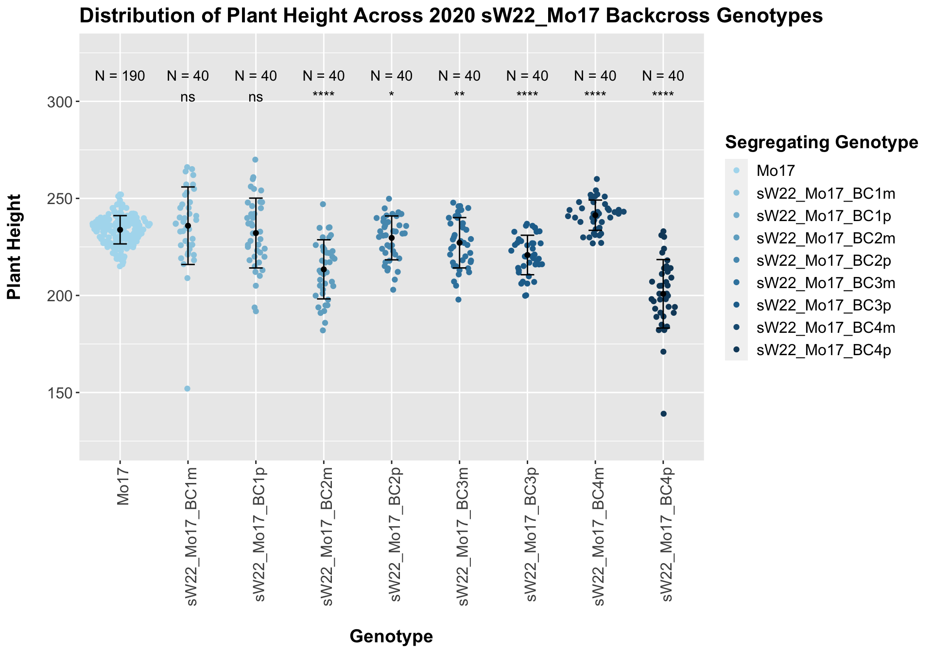
## # A tibble: 8 x 8
## .y. group1 group2 p p.adj p.format p.signif method
## <chr> <chr> <chr> <dbl> <dbl> <chr> <chr> <chr>
## 1 Plant_Height Mo17 sW22_Mo17_BC1m 5.17e- 1 1.00e+ 0 0.5168 ns T-test
## 2 Plant_Height Mo17 sW22_Mo17_BC1p 5.64e- 1 1.00e+ 0 0.5641 ns T-test
## 3 Plant_Height Mo17 sW22_Mo17_BC2m 2.05e-10 1.40e- 9 2.1e-10 **** T-test
## 4 Plant_Height Mo17 sW22_Mo17_BC2p 2.98e- 2 8.90e- 2 0.0298 * T-test
## 5 Plant_Height Mo17 sW22_Mo17_BC3m 2.87e- 3 1.10e- 2 0.0029 ** T-test
## 6 Plant_Height Mo17 sW22_Mo17_BC3p 7.23e-10 4.30e- 9 7.2e-10 **** T-test
## 7 Plant_Height Mo17 sW22_Mo17_BC4m 7.17e- 7 3.60e- 6 7.2e-07 **** T-test
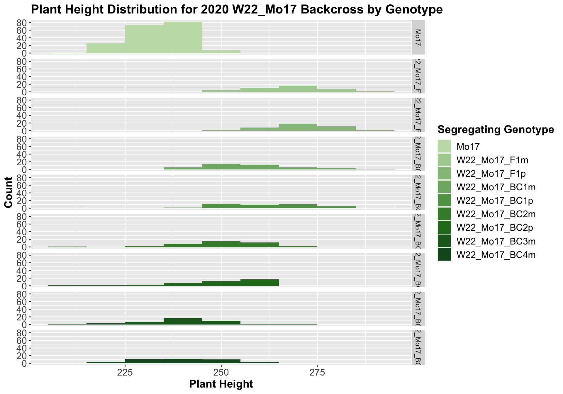
## 8 Plant_Height Mo17 sW22_Mo17_BC4p 1.13e-14 9.00e-14 1.1e-14 **** T-testHere, we see no increase in plant height among the F1s and both an incrase an decrease in plant height as we keep backcrossing to Mo17. We stratify the data by field to see whether this pattern is driven by one field.
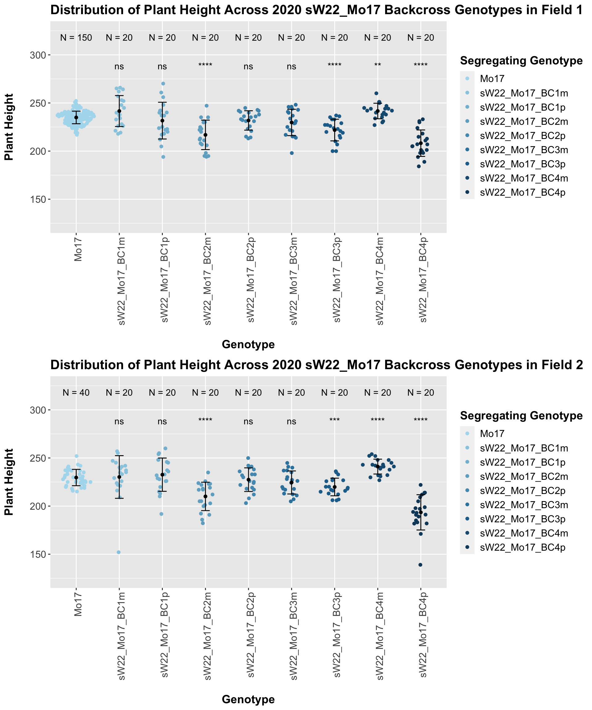
It does seem like when we stratify by field, the trend of an initial increase in plant height for the F1s followed by a continual decline in height emerges and maintains significance.
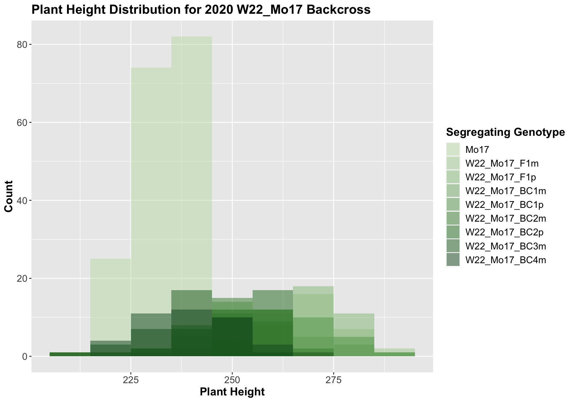
##
##  Mean, SD, and SE for each genotype
## Seg_Genotype N mean sd se
## 1 Mo17 190 233.8316 7.285054 0.5285134
## 2 W22_Mo17_F1m 40 268.6250 9.841533 1.5560830
## 3 W22_Mo17_F1p 40 271.0750 8.407529 1.3293470
## 4 W22_Mo17_BC1m 40 257.9750 12.613561 1.9943791
## 5 W22_Mo17_BC1p 40 260.7750 14.249584 2.2530570
## 6 W22_Mo17_BC2m 40 251.1500 11.002447 1.7396397
## 7 W22_Mo17_BC2p 40 250.4000 12.171425 1.9244713
## 8 W22_Mo17_BC3m 40 239.1500 9.874988 1.5613727
## 9 W22_Mo17_BC4m 40 239.5500 10.389714 1.6427580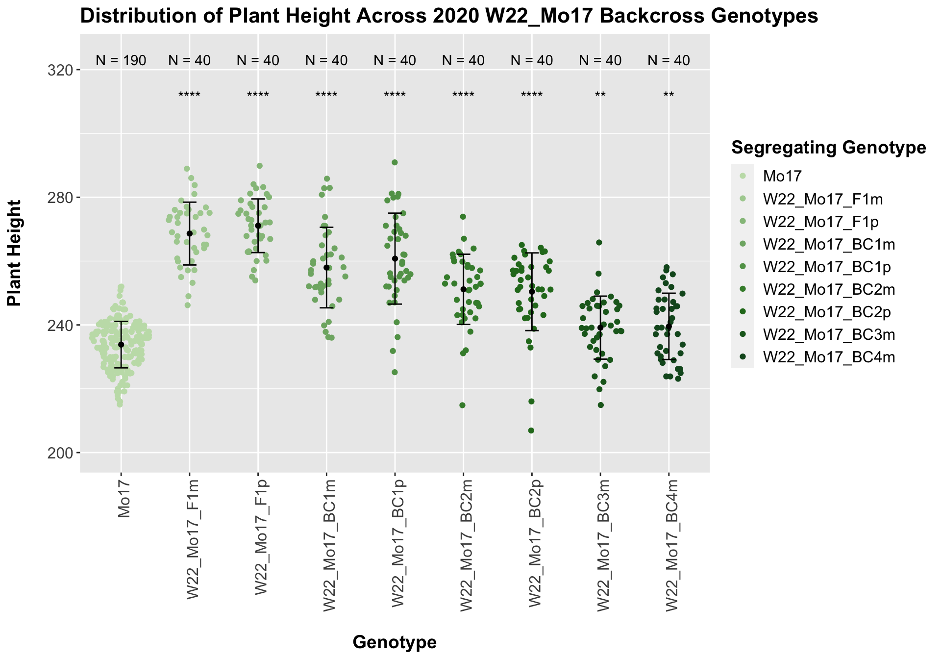
## # A tibble: 8 x 8
##   .y.          group1 group2               p    p.adj p.format p.signif method
##   <chr>        <chr>  <chr>            <dbl>    <dbl> <chr>    <chr>    <chr>
## 1 Plant_Height Mo17   W22_Mo17_F1m  4.10e-26 2.90e-25 < 2e-16  ****     T-test
## 2 Plant_Height Mo17   W22_Mo17_F1p  1.65e-31 1.30e-30 < 2e-16  ****     T-test
## 3 Plant_Height Mo17   W22_Mo17_BC1m 3.43e-15 2.10e-14 3.4e-15  ****     T-test
## 4 Plant_Height Mo17   W22_Mo17_BC1p 6.16e-15 3.10e-14 6.2e-15  ****     T-test
## 5 Plant_Height Mo17   W22_Mo17_BC2m 1.69e-12 6.80e-12 1.7e-12  ****     T-test
## 6 Plant_Height Mo17   W22_Mo17_BC2p 1.25e-10 3.70e-10 1.2e-10  ****     T-test
## 7 Plant_Height Mo17   W22_Mo17_BC3m 2.25e- 3 3.50e- 3 0.0023   **       T-test
## 8 Plant_Height Mo17   W22_Mo17_BC4m 1.77e- 3 3.50e- 3 0.0018   **       T-test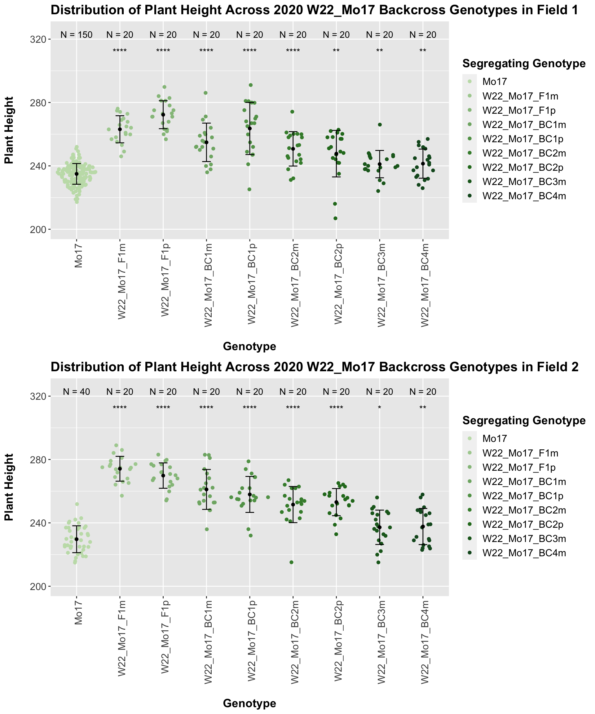
We see a very clear and significant trend for the W22 backcrossed to Mo17 where there is an intial increase in plant height followed by a continual decline in height as we continue backcrossing to Mo17.
We may compare how each generation compares across the sW22_Mo17 backcrosses to W22_Mo17 backcrosses. Note: when looking at these plots, just be aware that the genotypes don't align perfectly across backcrosses because we don't have a few crosses for the W22_B73 genotypes.
## List of 1
##  $ axis.text.x:List of 11
##   ..$ family       : NULL
##   ..$ face         : NULL
##   ..$ colour       : NULL
##   ..$ size         : NULL
##   ..$ hjust        : num 1
##   ..$ vjust        : num 0.75
##   ..$ angle        : num 90
##   ..$ lineheight   : NULL
##   ..$ margin       : NULL
##   ..$ debug        : NULL
##   ..$ inherit.blank: logi FALSE
##   ..- attr(*, "class")= chr [1:2] "element_text" "element"
##  - attr(*, "class")= chr [1:2] "theme" "gg"
##  - attr(*, "complete")= logi FALSE
##  - attr(*, "validate")= logi TRUE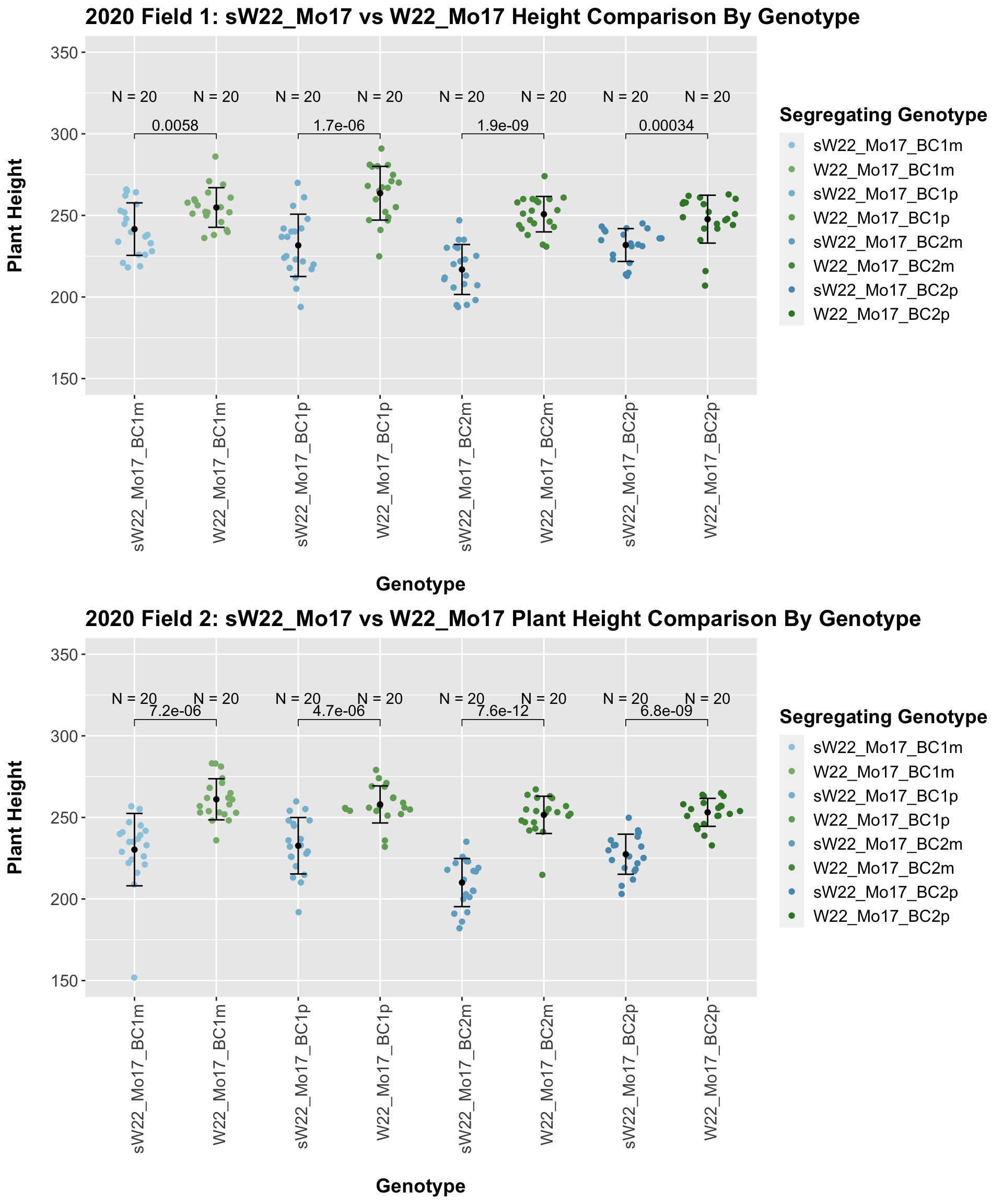
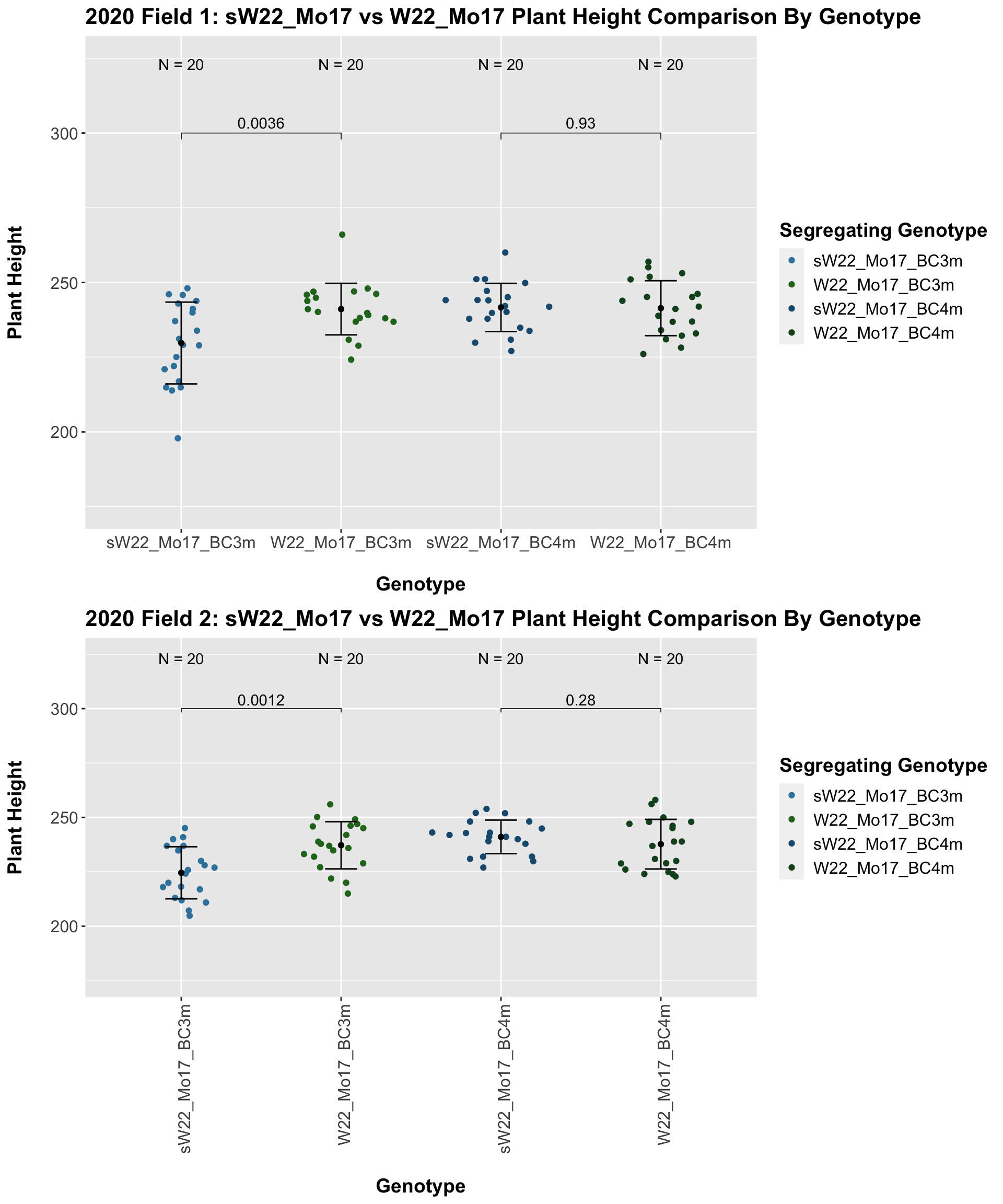
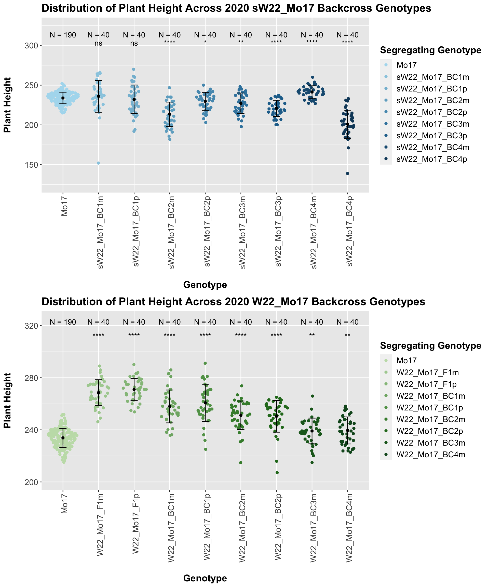
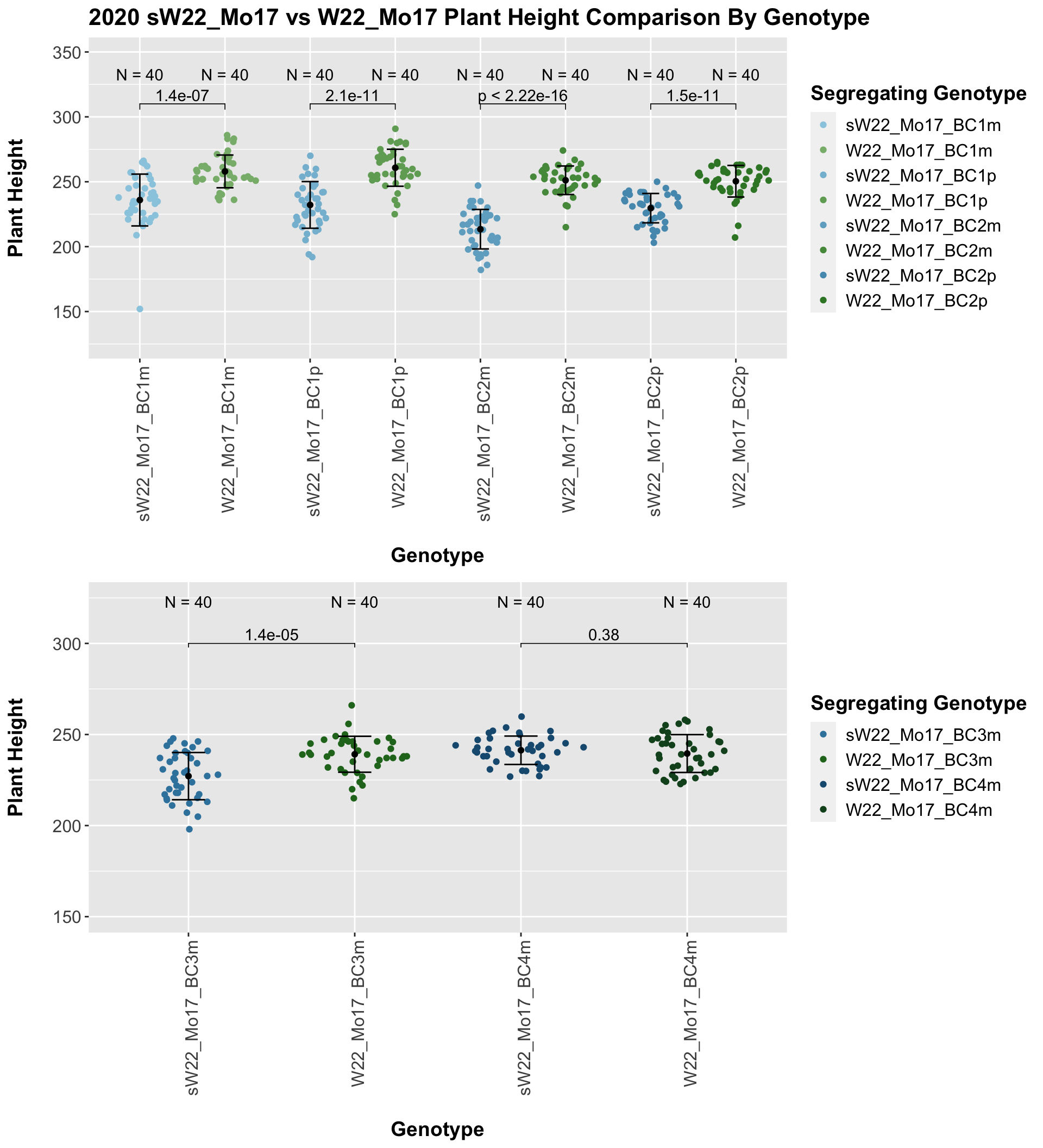
We see a consistent reduction in plant height for the sW22_Mo17 backcrosses in comparison to the W22_Mo17 backcrosses at each generation. This holds and even becomes more significant if we stratify the data by field.
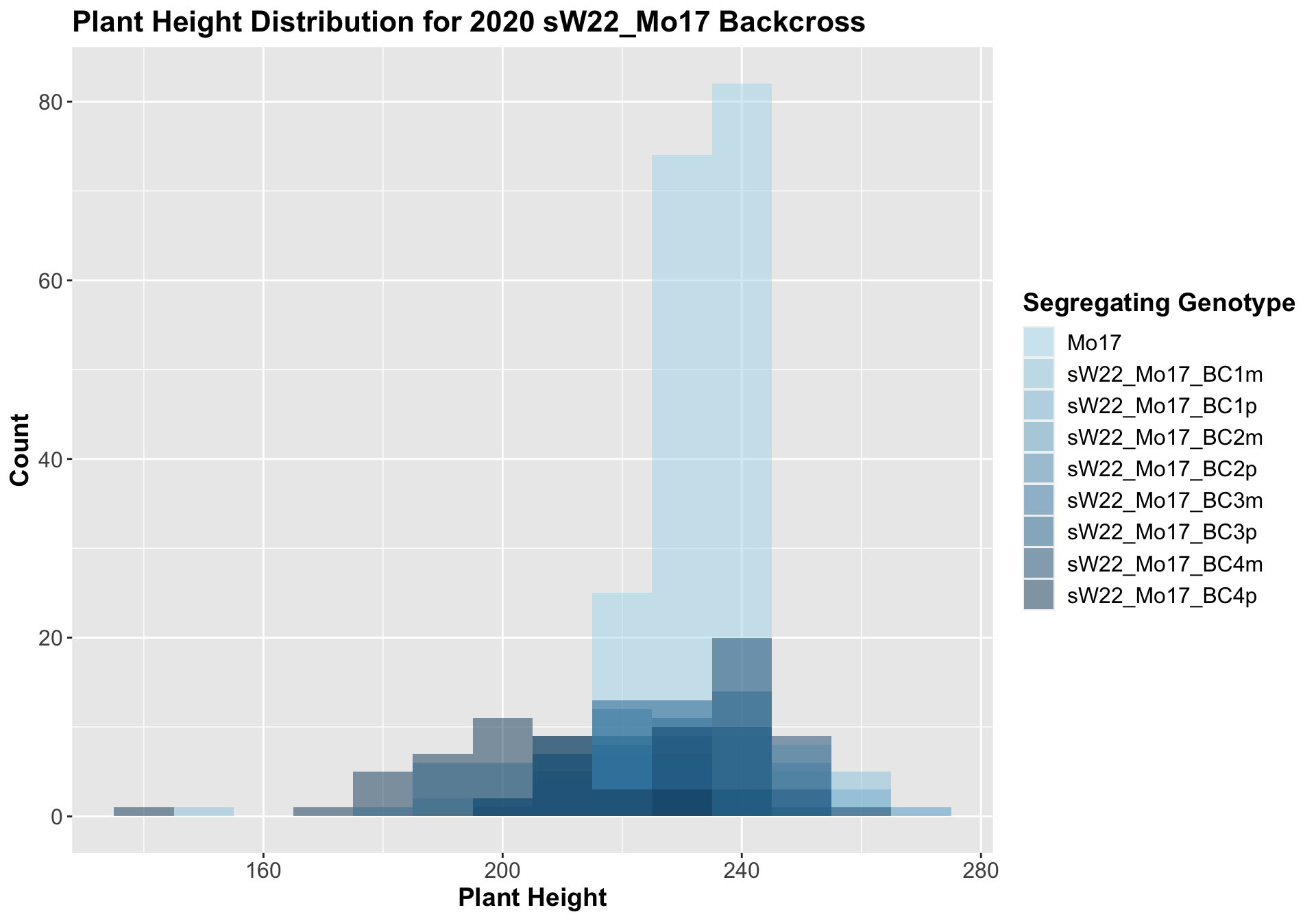
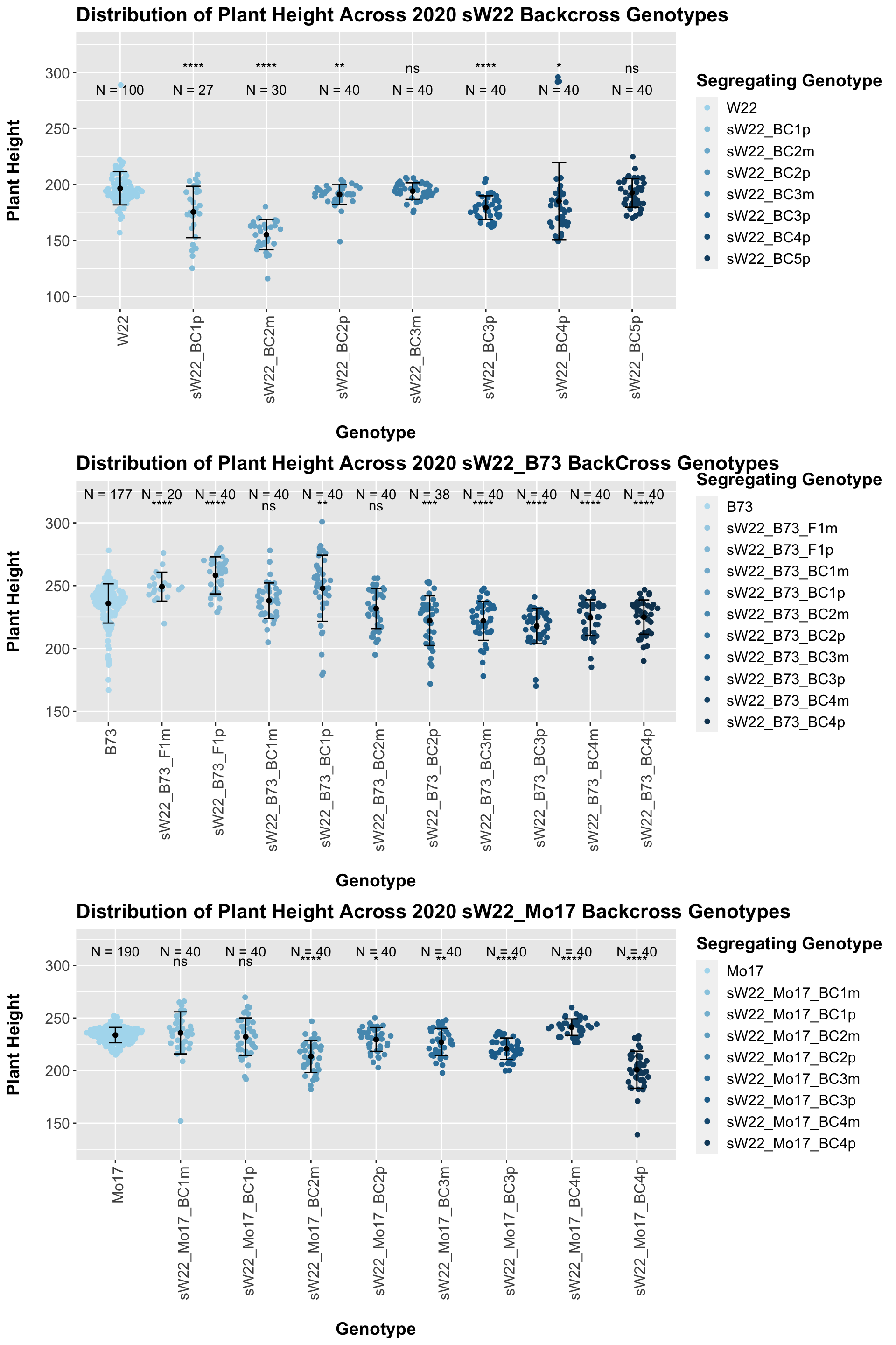
We may also be interested the distribution for all sW22 backcrosses (crossed to W22, B73, and Mo17 respectively). Note: when looking at these plots, just be aware that the genotypes don't align perfectly across backcrosses so be sure to check the x-axis.
3.2.4 2020 ANOVA for Plant Height
So far, we have only tested the difference of each segregating genotype against the external control it has been backcrossed to. We now want to test whether (1) ear height is impacted by the sex of the sick parent and (2) the means across each backcross generation change NOTE: I was not fully confident in how/whether to incorporate the external stock information (W22, B73,Mo17) as these lineages were selfed and therefore had no sick parent to test the sex of. We also transformed the categorical genotype values (F1,BC1,BC2,BC3,BC4,BC5) to numerical values (0,1,2,3,4,5). NOTE: I'm not sure if this is appropriate. It'd be fairly simple to switch this back to categorical values if that would be better
We start by fitting a series of linear models:
- mod_full_int: Plant_Height (Numerical) ~ Field (Cateogrical) + Genotype (Numerical) + Sick_Sex (Categorical) + Genotype*Sick_Sex
- mod_full: Plant_Height (Numerical) ~ Field (Categorical) + Genotype (Numerical) + Sick_Sex (Categorical)
- mod_geno: Plant_Height (Numerical) ~ Field (Cateogrical) + Genotype (Numerical)
- mod_sex: Plant_Height (Numerical) ~ Field + Sick_Sex (Categorical)
We can then compare the fit of these models to our data using an ANOVA to test whether the more complex model (mod_full) is significantly better at capturing our height data than either of our simpler models. This will tell us whether incorporating sex/genotype significantly improves our model.
We can summarize the results of this across each set of genotypes. The significance codes are as follows:
- '***' - between 0 and 0.001
- '**' - between 0.001 and 0.01
- '*' - between 0.01 and 0.05
- '.' - between 0.05 and 0.1
- ' ' - between 0.1 and 1
##    Geno_Set   Sex_PValue Sex_Signif Genotype_PValue Genotype_Signif
## 1  sW22_W22 7.082822e-02          .    1.280134e-05             ***
## 2  sW22_B73 4.649958e-01               4.400866e-31             ***
## 3 sW22_Mo17 2.407497e-05        ***    6.289803e-05             ***
## 4   W22_B73 1.457664e-20        ***    1.195814e-51             ***
## 5  W22_Mo17 3.508944e-01               3.174757e-41             ***
##   Sex_Geno_Int_PValue Sex_Geno_Int_Signif
## 1        3.081379e-15                 ***
## 2        5.400533e-03                  **
## 3        1.024255e-14                 ***
## 4        4.579576e-01
## 5        5.855155e-02                   .
We find that the genotype (i.e. the number of backcrosses to the external stock) consistently improves prediction of plant height. However, we do not find that the sex of the sick parent consistently improves prediction. The two sets of genotypes where the sex of the sick parent is significant is sW22_Mo17 and W22_B73. We also find that there is consistently an interaction between the sex of the sick parent and the genotype on improving the prediction of plant height.