Chapter 7 Cobb Weight
7.1 2019 Cobb Weight Data
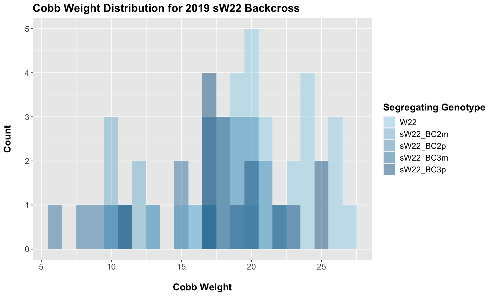
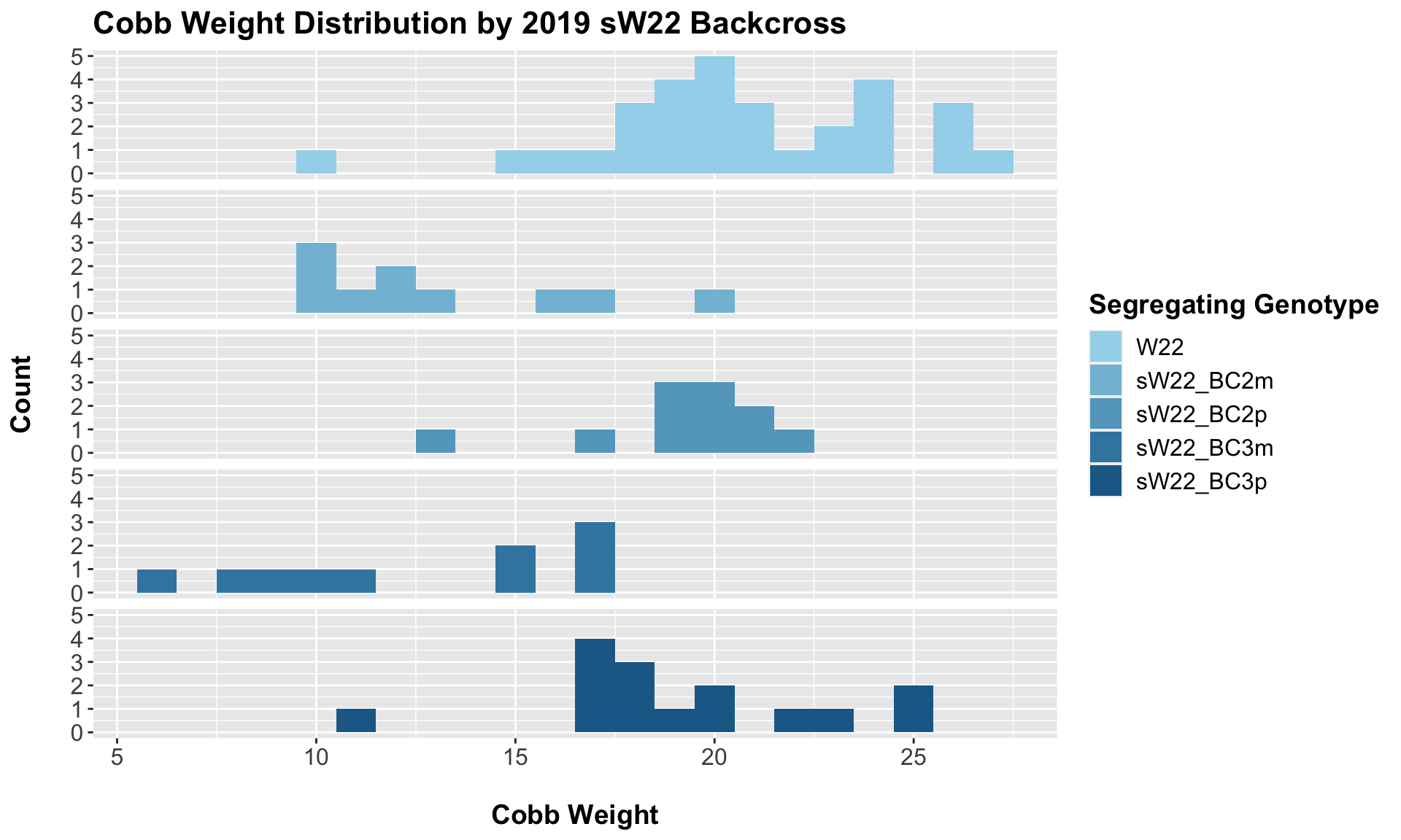
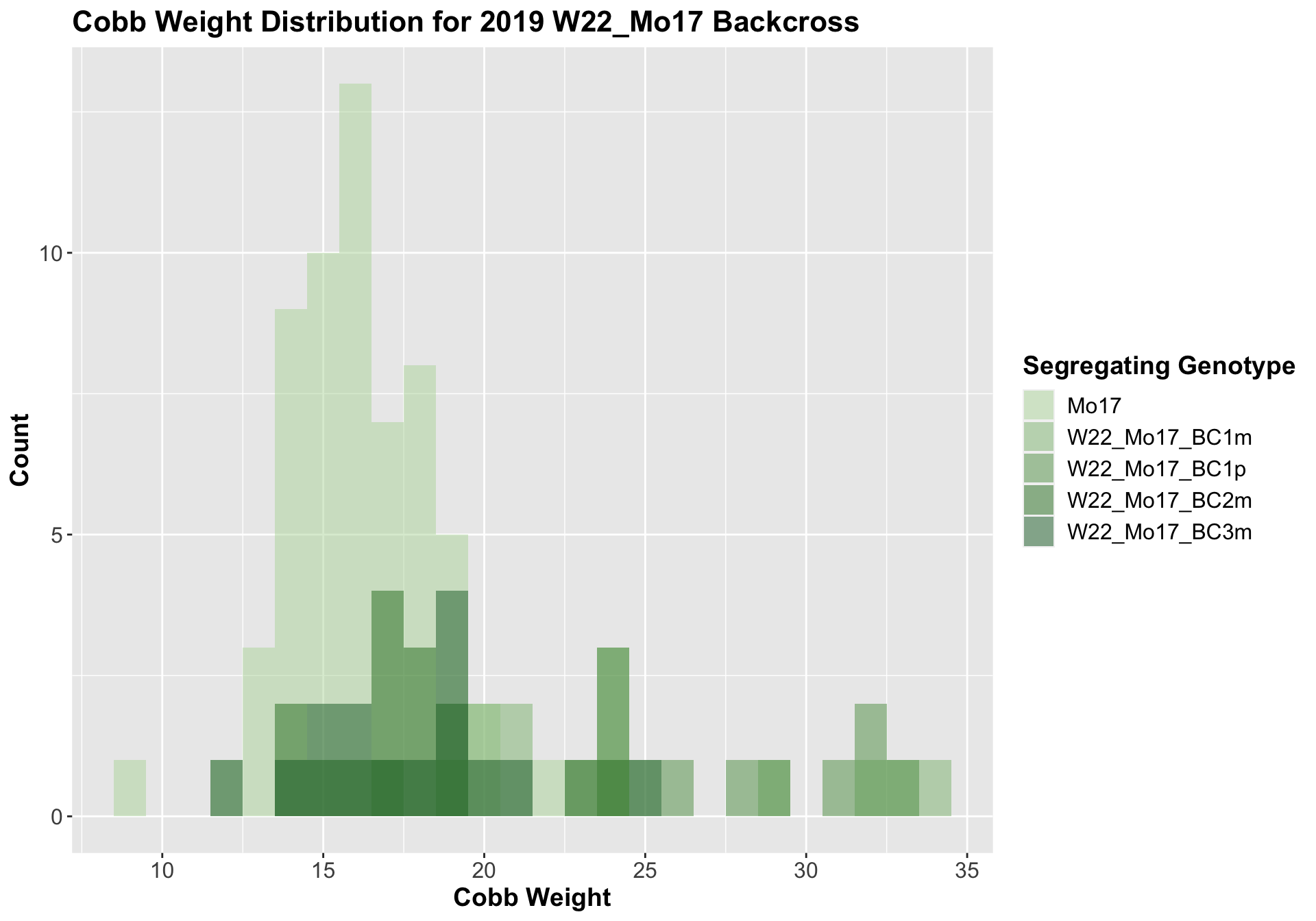
7.1.1 2019 sW22 backcrossed to W22
##
##  Mean, SD, and SE for each genotype
## Seg_Genotype N mean sd se
## 1 W22 30 20.70000 3.656831 0.6676430
## 2 sW22_BC2m 10 13.20000 3.400980 1.0754844
## 3 sW22_BC2p 11 19.45455 2.413033 0.7275568
## 4 sW22_BC3m 10 12.60000 4.081122 1.2905640
## 5 sW22_BC3p 15 19.30000 3.544614 0.9152153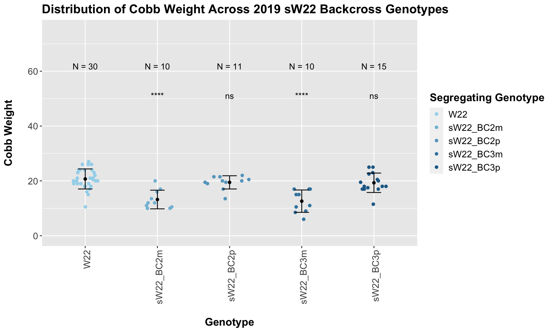
##
## Results of T-test used to obtain significance in the above plot
## # A tibble: 4 x 8
## .y. group1 group2 p p.adj p.format p.signif method
## <chr> <chr> <chr> <dbl> <dbl> <chr> <chr> <chr>
## 1 Ear_Trait W22 sW22_BC2m 0.0000188 0.000075 1.9e-05 **** T-test
## 2 Ear_Trait W22 sW22_BC2p 0.218 0.44 0.22 ns T-test
## 3 Ear_Trait W22 sW22_BC3m 0.0000659 0.0002 6.6e-05 **** T-test
## 4 Ear_Trait W22 sW22_BC3p 0.226 0.44 0.23 ns T-testWe find that the cobb weight of our sW22 backcrosses is lower than that of the W22 if the maternal parent was sick. If the paternal parent was sick, we find that it has a heavier cobb weight that is not signficantly different from the W22 weight. We can check whether this pattern holds across both fields or if it is driven by one.
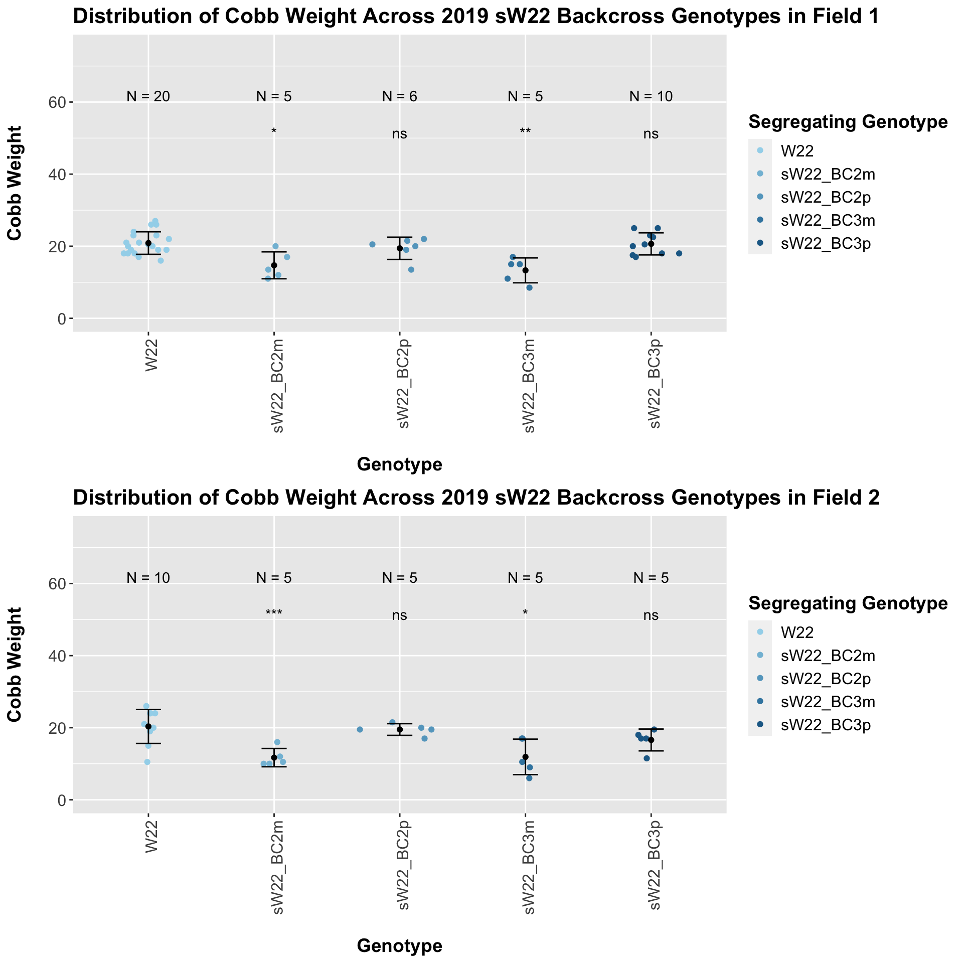
This trend holds when we separate the data by field. This is another example of where the phenotype of the paternal sick parent is elevated (and consequently more similar to the W22) compared to the phenotype of the maternal sick parent.
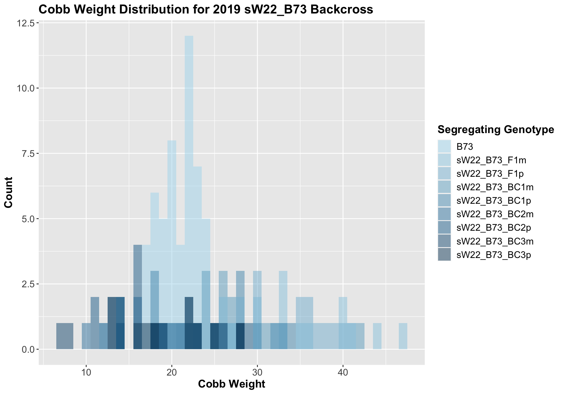
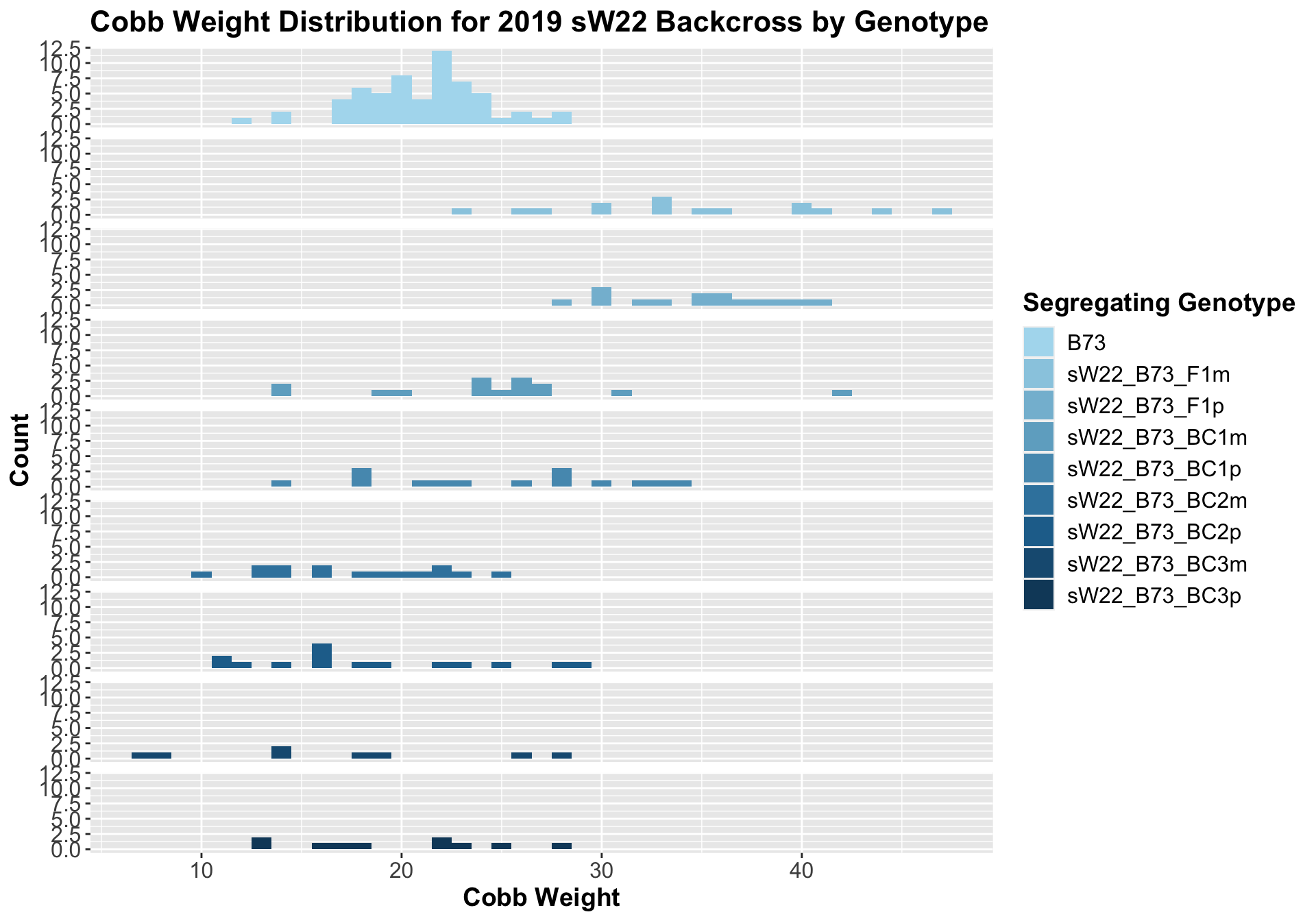
7.1.2 2019 sW22 and W22 backcrossed to W22
##
##  Mean, SD, and SE for each genotype
## Seg_Genotype N mean sd se
## 1 B73 60 21.08333 3.194496 0.4124076
## 2 sW22_B73_F1m 15 34.60000 6.798634 1.7553998
## 3 sW22_B73_F1p 15 34.70000 4.078690 1.0531133
## 4 sW22_B73_BC1m 15 24.70000 6.747486 1.7421935
## 5 sW22_B73_BC1p 15 24.93333 6.264602 1.6175133
## 6 sW22_B73_BC2m 15 17.80000 4.447311 1.1482907
## 7 sW22_B73_BC2p 15 18.53333 5.780097 1.4924147
## 8 sW22_B73_BC3m 8 16.81250 7.717964 2.7287122
## 9 sW22_B73_BC3p 10 19.75000 5.105825 1.6146035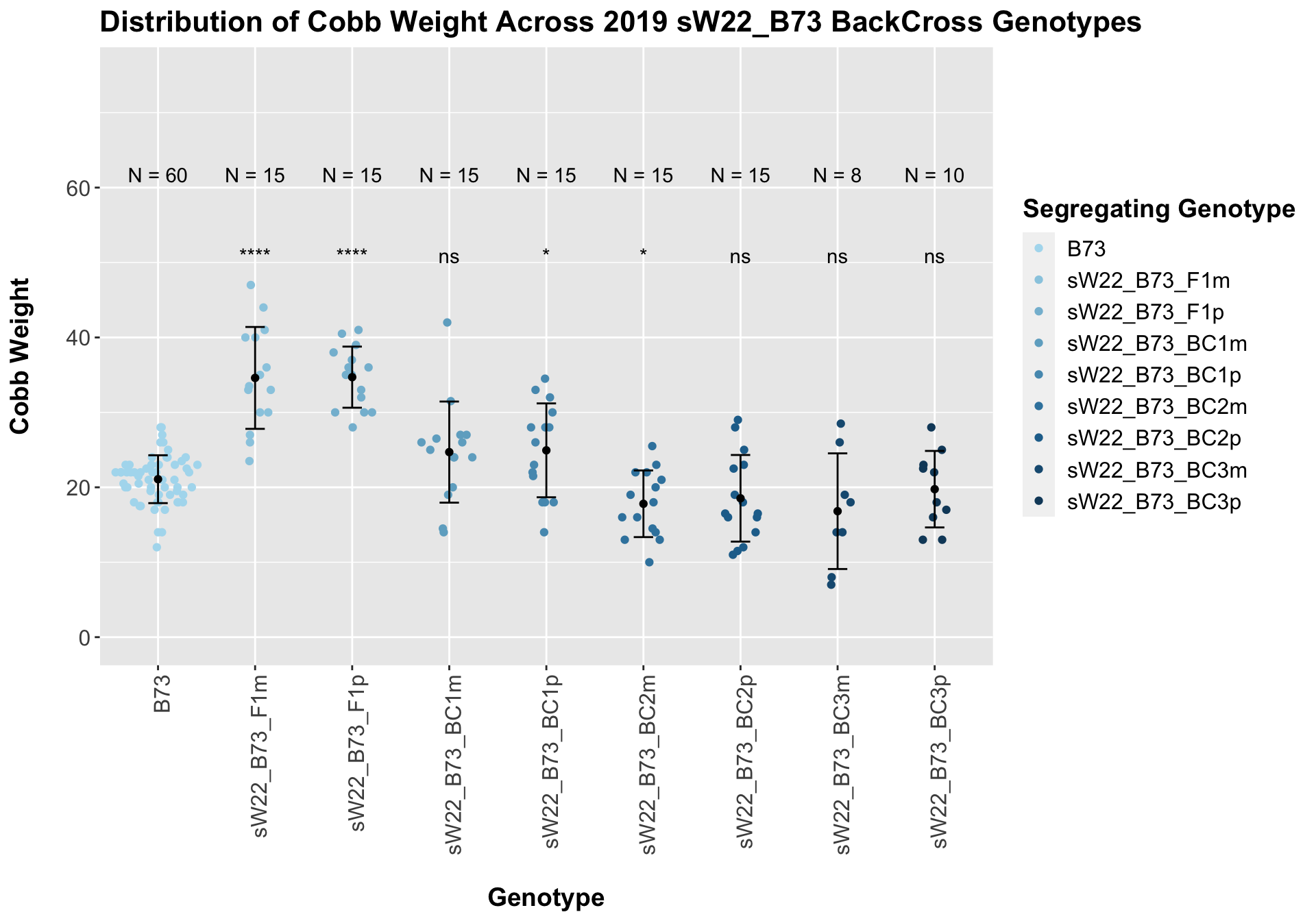
## # A tibble: 8 x 8
## .y. group1 group2 p p.adj p.format p.signif method
## <chr> <chr> <chr> <dbl> <dbl> <chr> <chr> <chr>
## 1 Ear_Trait B73 sW22_B73_F1m 1.51e- 6 0.000011 1.5e-06 **** T-test
## 2 Ear_Trait B73 sW22_B73_F1p 3.37e-10 0.0000000027 3.4e-10 **** T-test
## 3 Ear_Trait B73 sW22_B73_BC1m 6.09e- 2 0.24 0.061 ns T-test
## 4 Ear_Trait B73 sW22_B73_BC1p 3.49e- 2 0.17 0.035 * T-test
## 5 Ear_Trait B73 sW22_B73_BC2m 1.50e- 2 0.09 0.015 * T-test
## 6 Ear_Trait B73 sW22_B73_BC2p 1.19e- 1 0.36 0.119 ns T-test
## 7 Ear_Trait B73 sW22_B73_BC3m 1.64e- 1 0.36 0.164 ns T-test
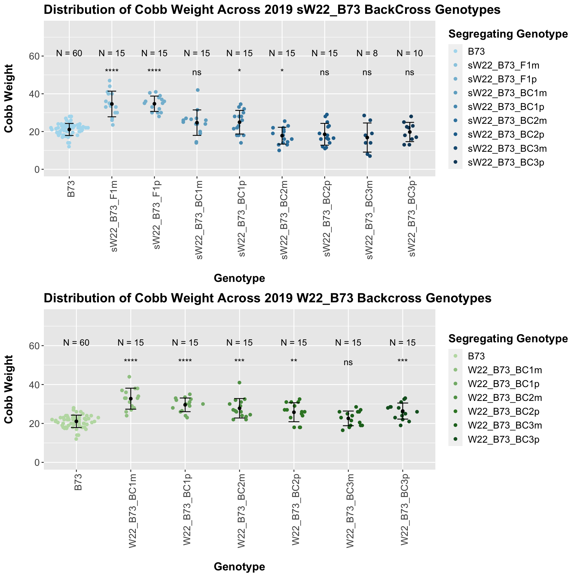
## 8 Ear_Trait B73 sW22_B73_BC3p 4.42e- 1 0.44 0.442 ns T-testWe see a marked increase in cobb weight for the sW22_B73 F1s that declines until it is not significantly different from the B73 weight. For the most part, we do not see a major difference within a generation between the sick maternal and paternal cross.
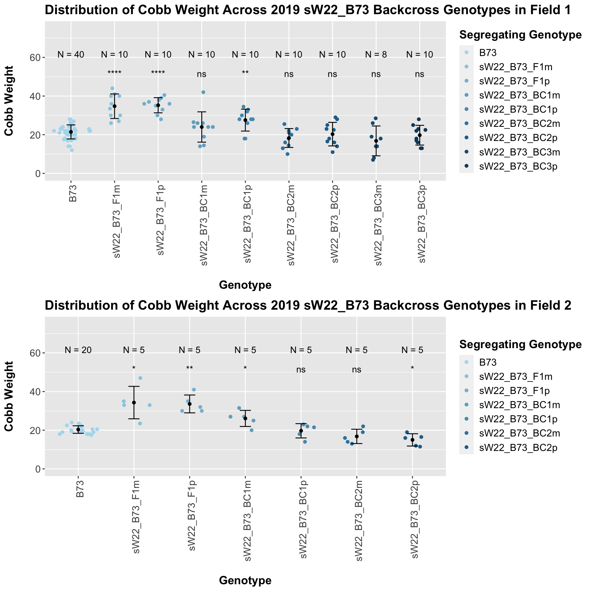
There is no noticeable difference between the trend and significance levels when we separte the data by field. We can compare the weight data across the W22 backcrossed to B73 rows to look at this set of controls.
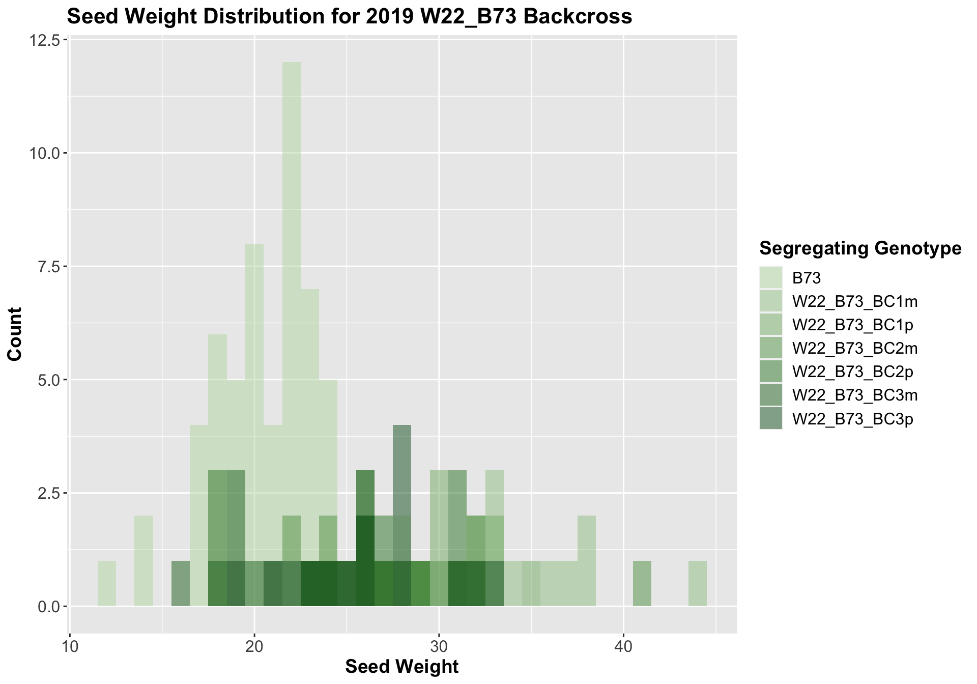
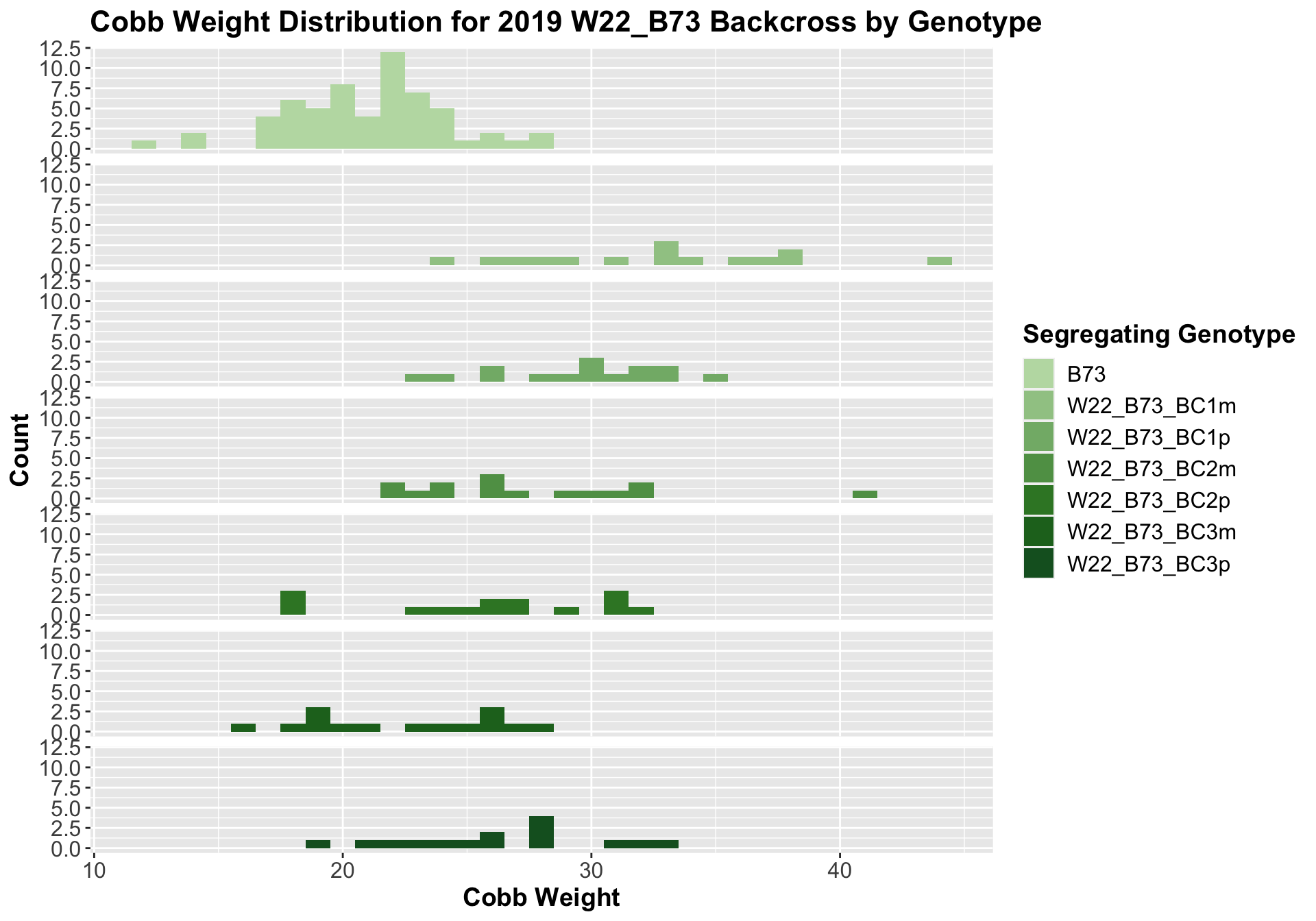
##
##  Mean, SD, and SE for each genotype
## Seg_Genotype N mean sd se
## 1 B73 60 21.08333 3.194496 0.4124076
## 2 W22_B73_BC1m 15 32.73333 5.391351 1.3920409
## 3 W22_B73_BC1p 15 29.56667 3.514595 0.9074646
## 4 W22_B73_BC2m 15 27.80000 5.002856 1.2917319
## 5 W22_B73_BC2p 15 25.76667 4.880232 1.2600705
## 6 W22_B73_BC3m 15 22.60000 3.775863 0.9749237
## 7 W22_B73_BC3p 15 26.36667 4.129453 1.0662201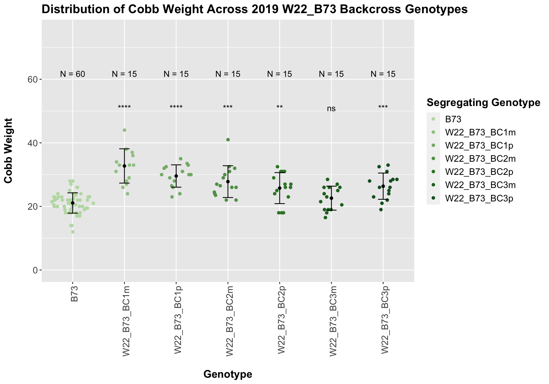
## # A tibble: 6 x 8
##   .y.       group1 group2                  p      p.adj p.format p.signif method
##   <chr>     <chr>  <chr>               <dbl>      <dbl> <chr>    <chr>    <chr>
## 1 Ear_Trait B73    W22_B73_BC1m 0.000000425  0.00000210 4.2e-07  ****     T-test
## 2 Ear_Trait B73    W22_B73_BC1p 0.0000000413 0.00000025 4.1e-08  ****     T-test
## 3 Ear_Trait B73    W22_B73_BC2m 0.000122     0.00049    0.00012  ***      T-test
## 4 Ear_Trait B73    W22_B73_BC2p 0.00254      0.0051     0.00254  **       T-test
## 5 Ear_Trait B73    W22_B73_BC3m 0.168        0.17       0.16792  ns       T-test
## 6 Ear_Trait B73    W22_B73_BC3p 0.000201     0.000600   0.00020  ***      T-test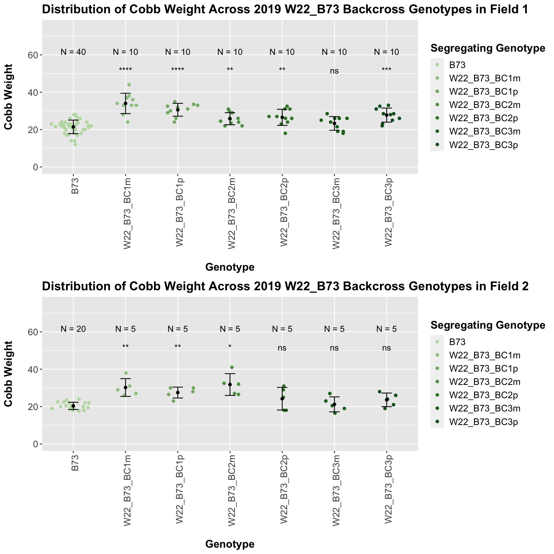
We see an increase in cobb weight among the F1s that declines across subsequent backcrosses. In Field 1, it seems as if the cobb weight in the later generation backcrosses is still higher when compared to the B73 cobb weight, while it is not significantly different in field 2.
We may also compare the distribution for sW22_B73 backcrosses to W22_B73 backcrosses and each generation compares across these two sets. Note: when looking at these plots, just be aware that the genotypes don't align perfectly across backcrosses because we don't have a few crosses for the W22_B73 genotypes.
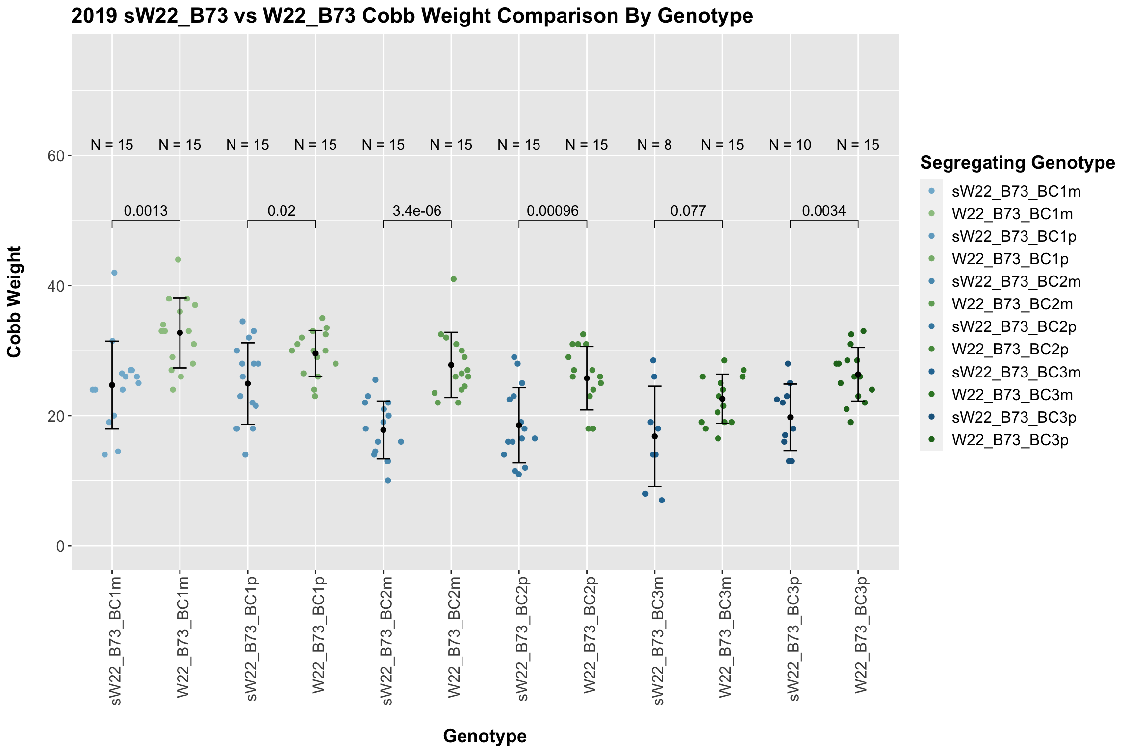
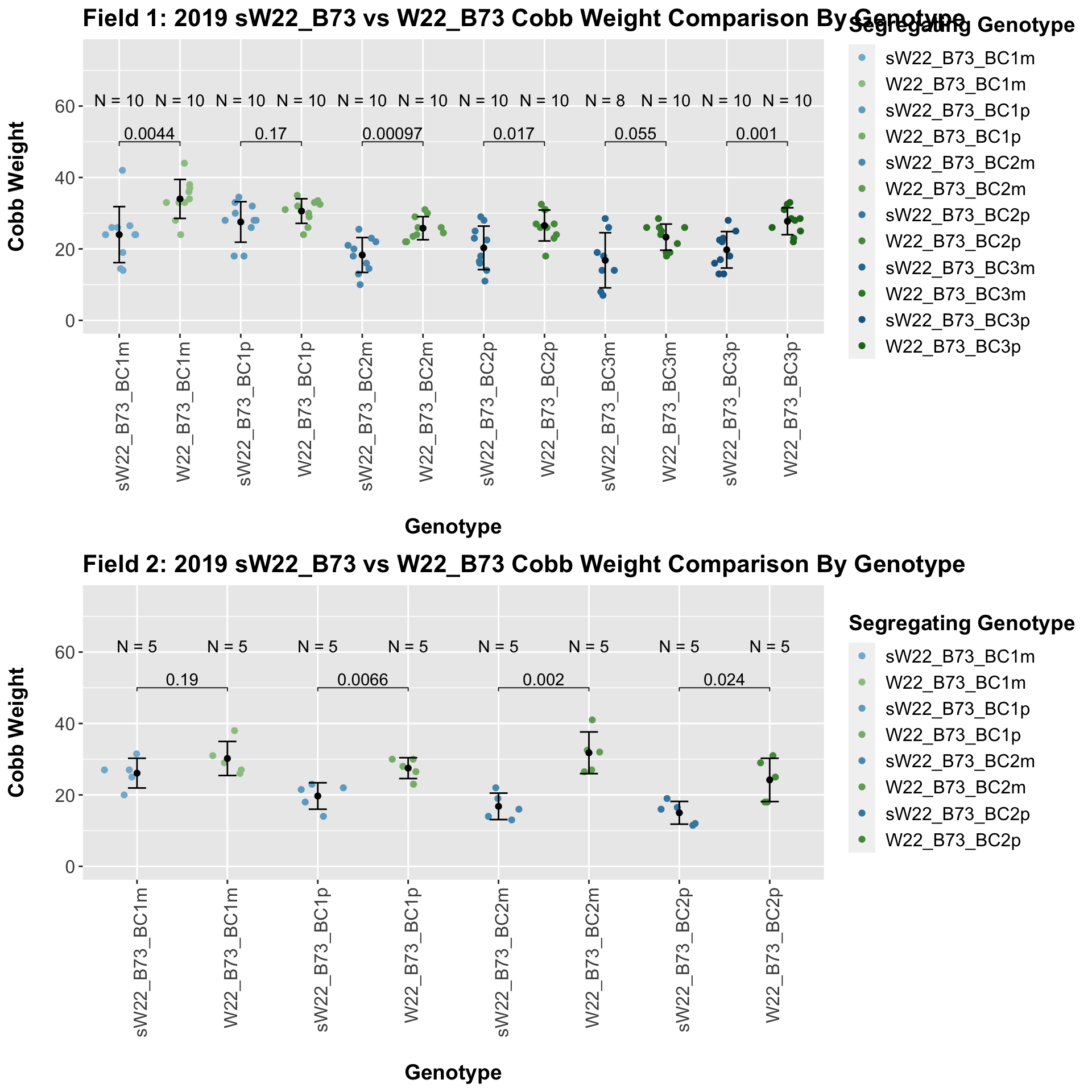
We find a significant reduction in cobb weight of the sW22_B73 backcrosses against the W22_B73 backcrosses. We find that this persists even when we stratify the data by field.
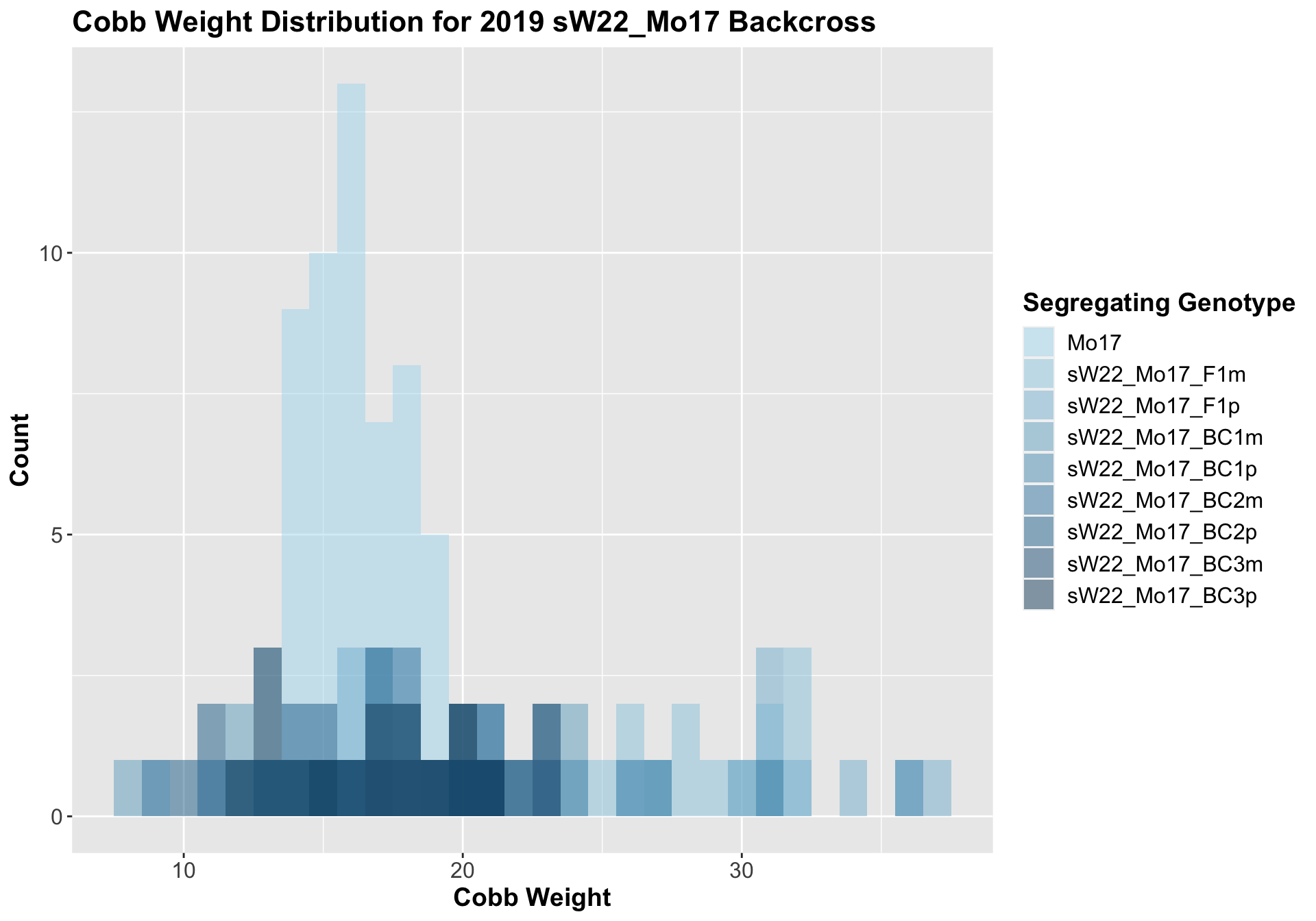
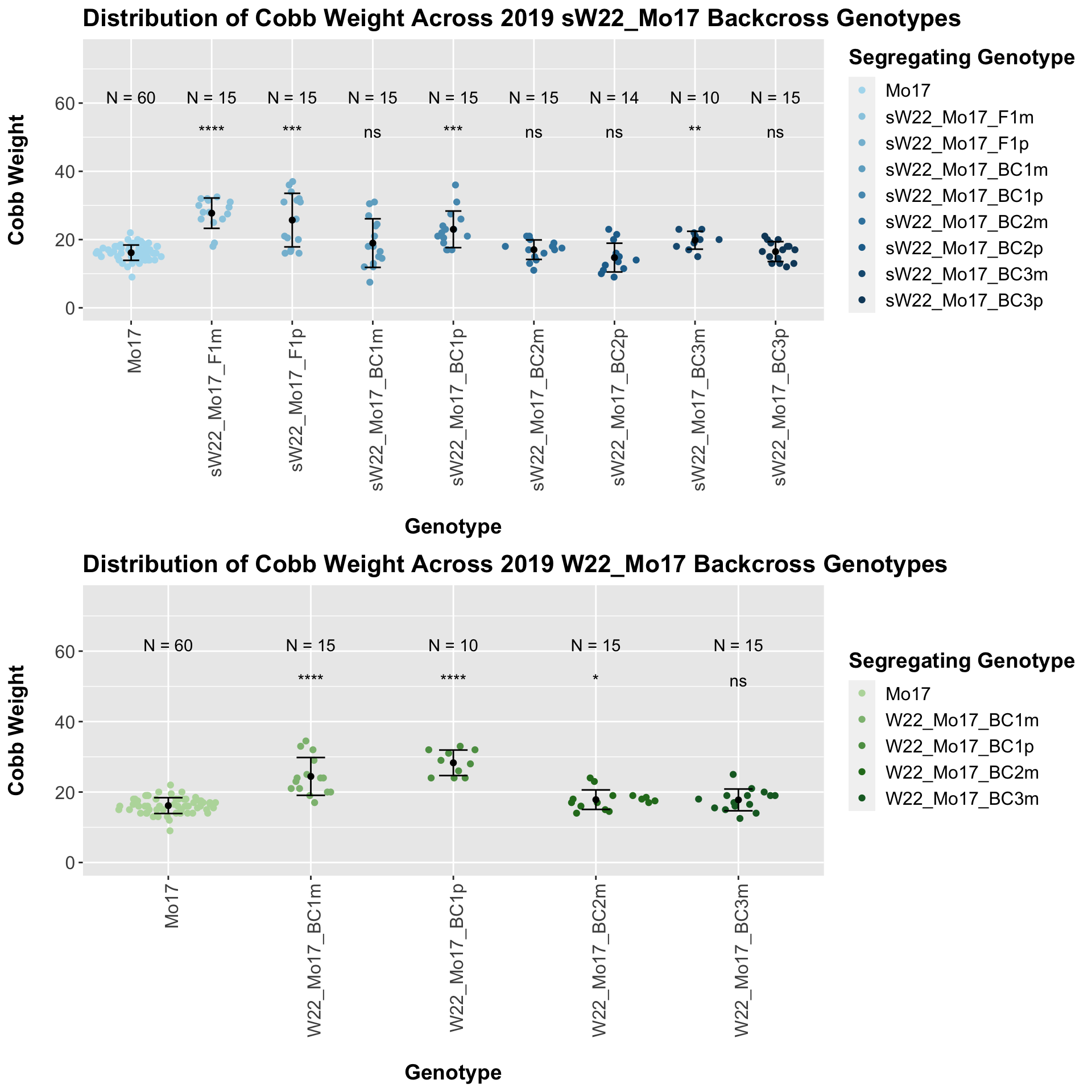
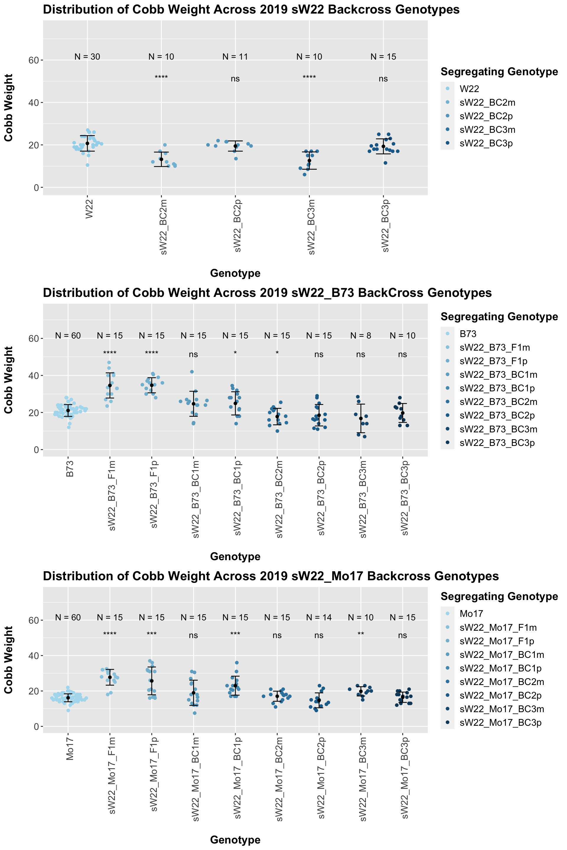
7.1.3 2019 sW22 and W22 backcrossed to Mo17
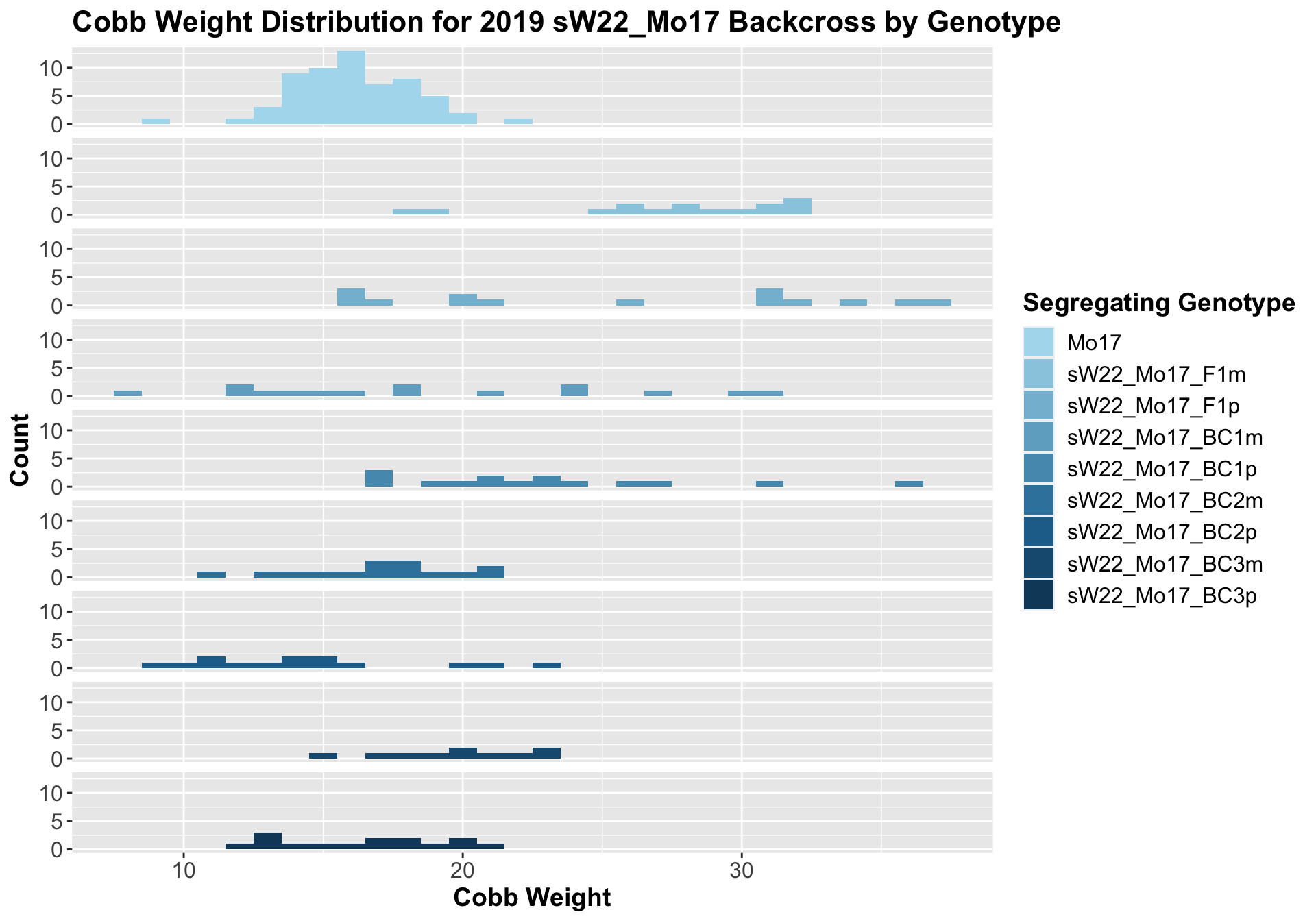
##
##  Mean, SD, and SE for each genotype
## Seg_Genotype N mean sd se
## 1 Mo17 60 16.15000 2.244202 0.2897252
## 2 sW22_Mo17_F1m 15 27.73333 4.447578 1.1483598
## 3 sW22_Mo17_F1p 15 25.70000 7.848567 2.0264912
## 4 sW22_Mo17_BC1m 15 18.96667 7.122566 1.8390387
## 5 sW22_Mo17_BC1p 15 23.00000 5.361903 1.3844373
## 6 sW22_Mo17_BC2m 15 17.03333 2.856488 0.7375420
## 7 sW22_Mo17_BC2p 14 14.71429 4.214053 1.1262530
## 8 sW22_Mo17_BC3m 10 19.80000 2.616189 0.8273116
## 9 sW22_Mo17_BC3p 15 16.46667 2.918333 0.7535103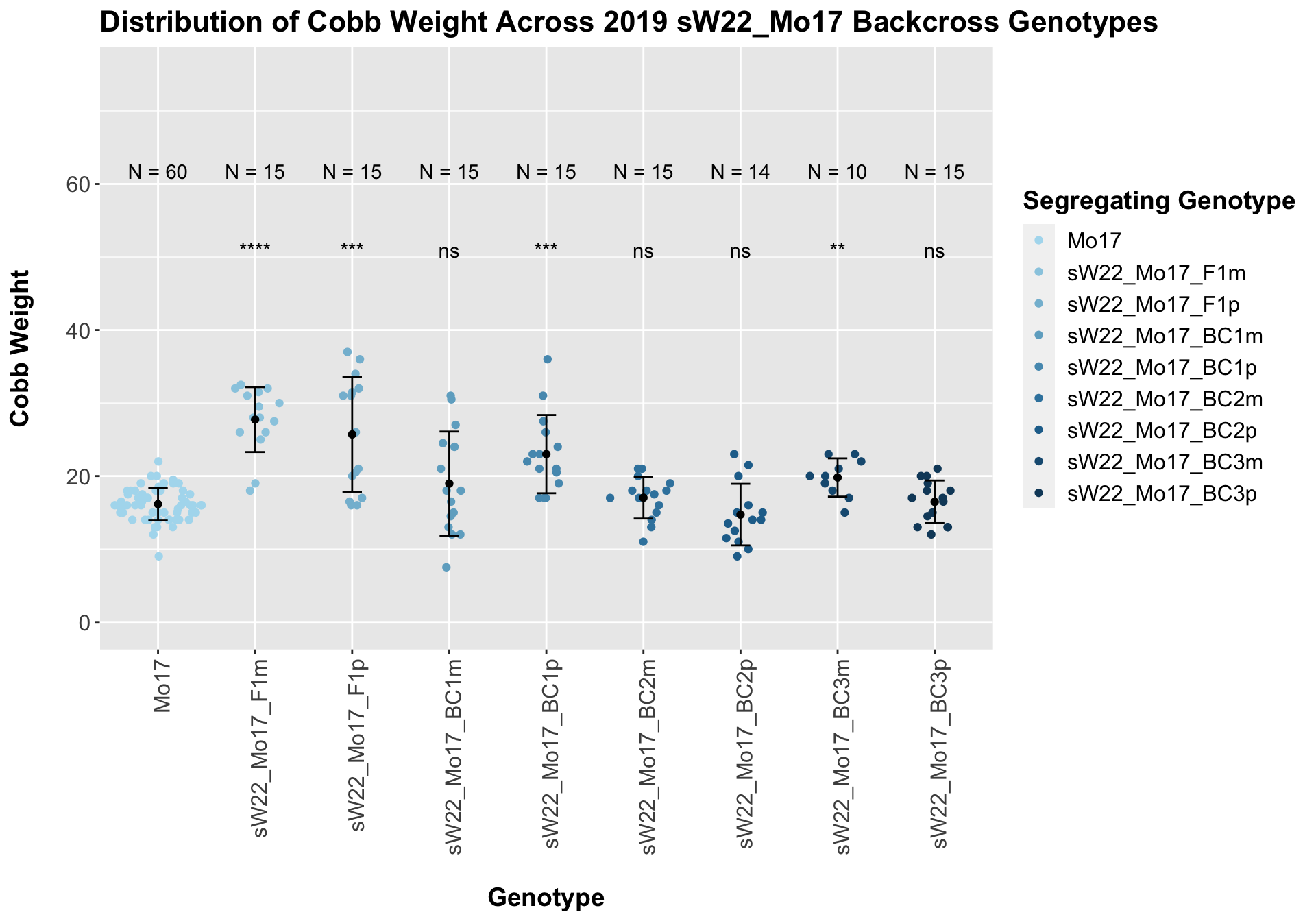
## # A tibble: 8 x 8
##   .y.       group1 group2                   p     p.adj p.format p.signif method
##   <chr>     <chr>  <chr>                <dbl>     <dbl> <chr>    <chr>    <chr>
## 1 Ear_Trait Mo17   sW22_Mo17_F1m      4.13e-8   3.30e-7 4.1e-08  ****     T-test
## 2 Ear_Trait Mo17   sW22_Mo17_F1p      3.28e-4   2.00e-3 0.00033  ***      T-test
## 3 Ear_Trait Mo17   sW22_Mo17_BC1m     1.51e-1   6.10e-1 0.15149  ns       T-test
## 4 Ear_Trait Mo17   sW22_Mo17_BC1p     2.06e-4   1.40e-3 0.00021  ***      T-test
## 5 Ear_Trait Mo17   sW22_Mo17_BC2m     2.79e-1   7.10e-1 0.27919  ns       T-test
## 6 Ear_Trait Mo17   sW22_Mo17_BC2p     2.36e-1   7.10e-1 0.23628  ns       T-test
## 7 Ear_Trait Mo17   sW22_Mo17_BC3m     1.49e-3   7.40e-3 0.00149  **       T-test
## 8 Ear_Trait Mo17   sW22_Mo17_BC3p     6.99e-1   7.10e-1 0.69939  ns       T-test
We see a significant increase in cobb weight at the sW22_Mo17 F1s that declines across subsequent backcrosses. By the later generations, it is not that different from the Mo17 cobb weight. This is similar to what we saw for the sW22_B73 backcross.
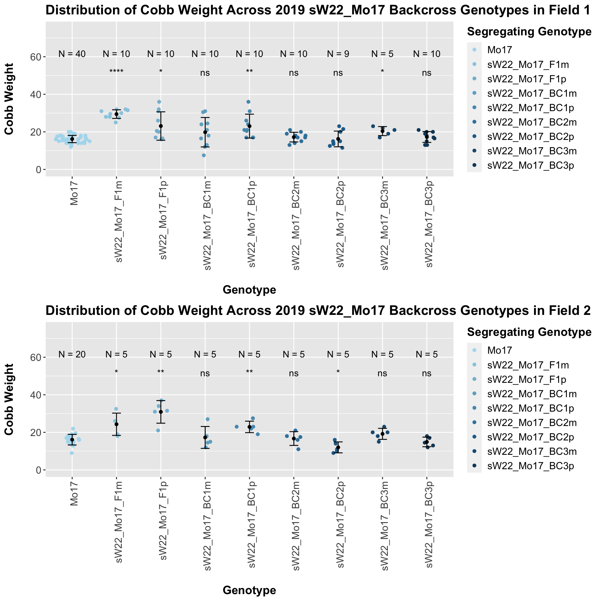
The pattern we saw holds when we seperate the data by field. We can compare the height data across the W22 backcrossed to Mo17 rows.
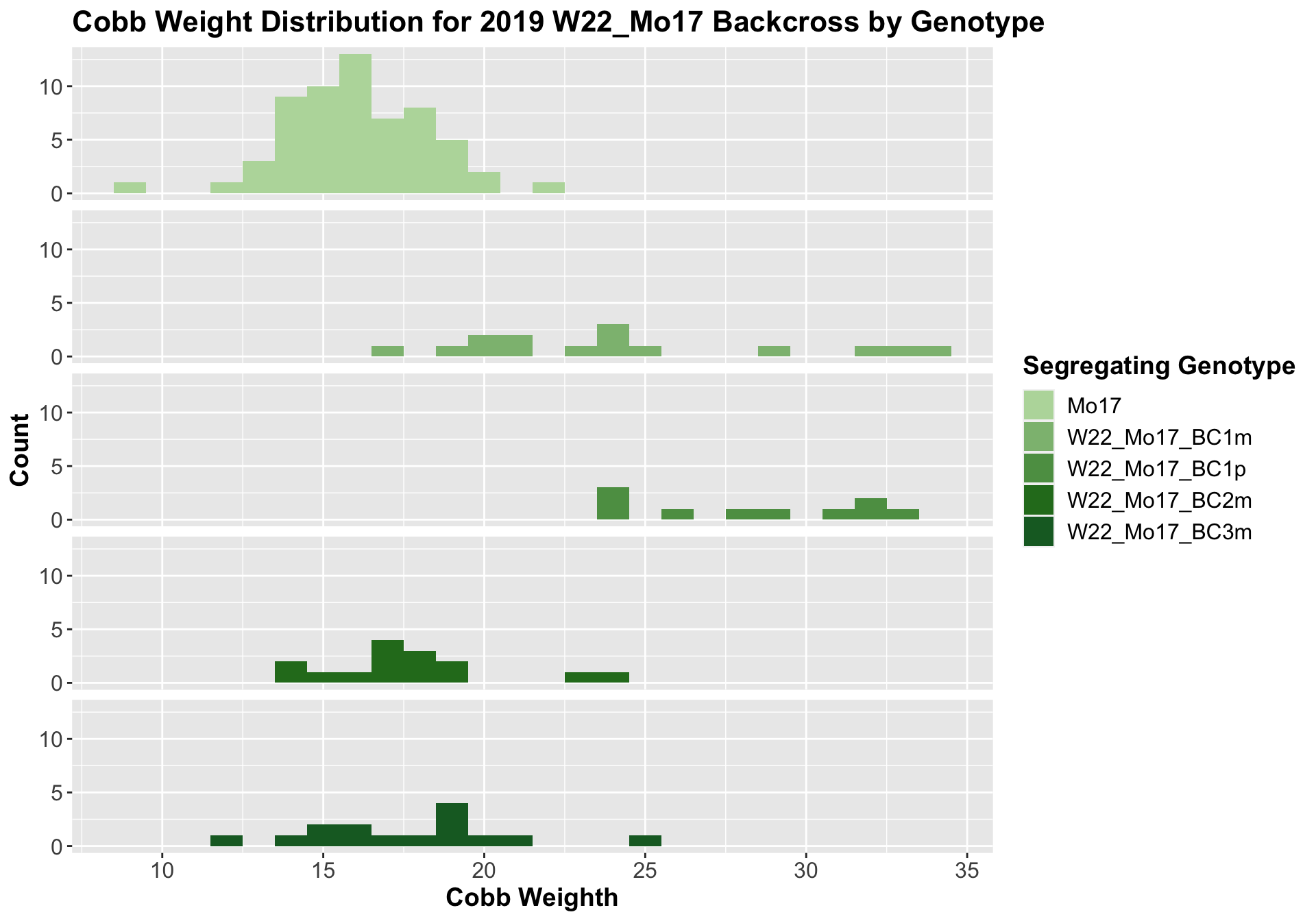
##
##  Mean, SD, and SE for each genotype
## Seg_Genotype N mean sd se
## 1 Mo17 60 16.15000 2.244202 0.2897252
## 2 W22_Mo17_BC1m 15 24.43333 5.368116 1.3860415
## 3 W22_Mo17_BC1p 10 28.30000 3.622461 1.1455227
## 4 W22_Mo17_BC2m 15 17.83333 2.768875 0.7149204
## 5 W22_Mo17_BC3m 15 17.76667 3.093003 0.7986099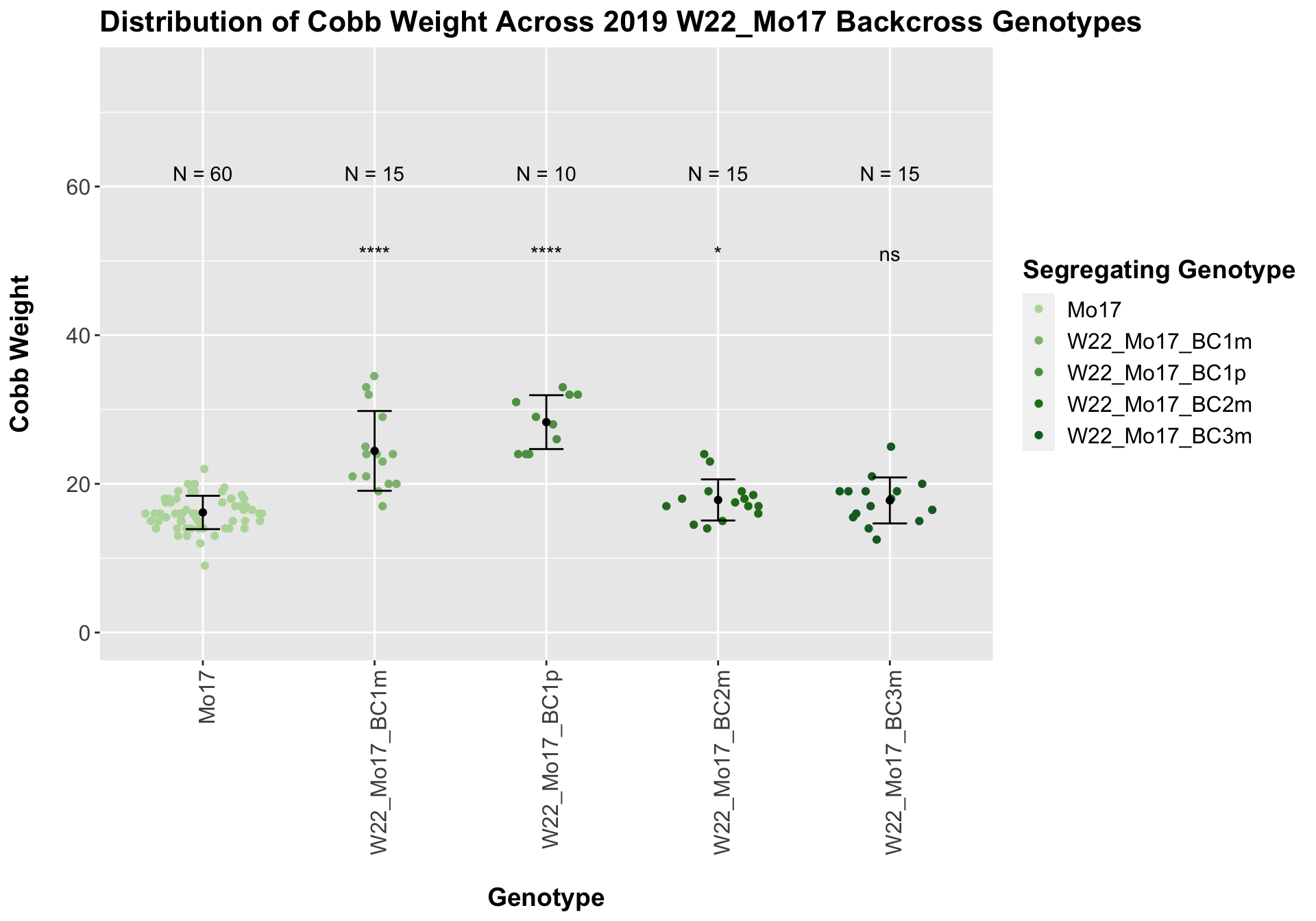
## # A tibble: 4 x 8
##   .y.       group1 group2                 p      p.adj p.format p.signif method
##   <chr>     <chr>  <chr>              <dbl>      <dbl> <chr>    <chr>    <chr>
## 1 Ear_Trait Mo17   W22_Mo17_BC1m 0.0000300  0.00009    3.0e-05  ****     T-test
## 2 Ear_Trait Mo17   W22_Mo17_BC1p 0.00000106 0.00000420 1.1e-06  ****     T-test
## 3 Ear_Trait Mo17   W22_Mo17_BC2m 0.0420     0.084      0.042    *        T-test
## 4 Ear_Trait Mo17   W22_Mo17_BC3m 0.0733     0.084      0.073    ns       T-test
We see a signficant increase in cobb weight for the first generation backcross that declines until there is no difference in weight when comapred to Mo17. This is even more pronounced when we seperate the data by field.
We now compare the distribution for sW22_Mo17 backcrosses to W22_Mo17 backcrosses and how each generaiton compares across these two sets. Note: when looking at these plots, just be aware that the genotypes don't align perfectly across backcrosses because we don't have a few crosses for the W22_Mo17 genotypes.
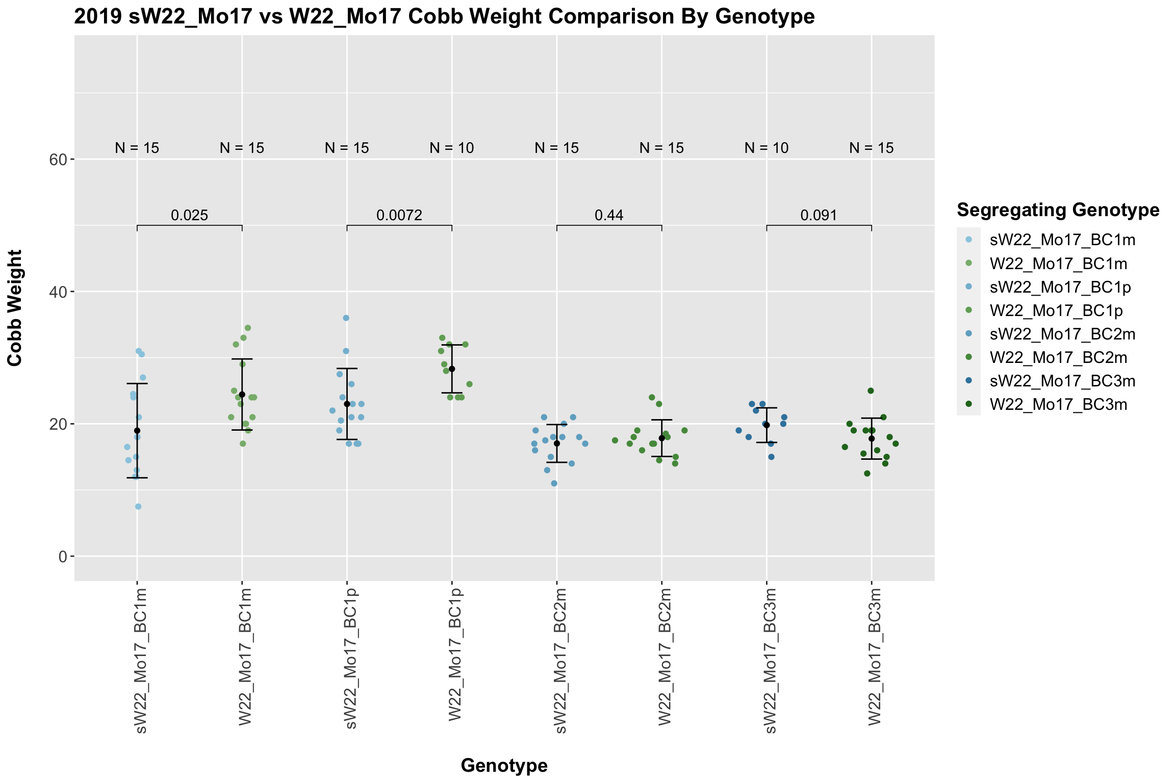
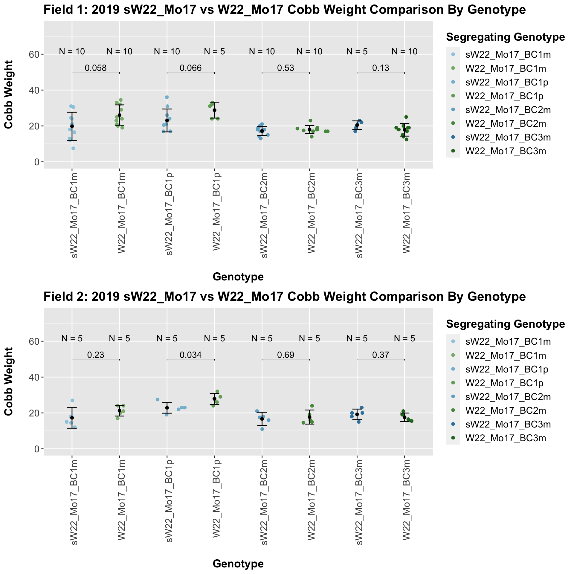
When we first look at the data, it seems that there is a significant difference in cobb weight between the sW22_Mo17 and W22_Mo17 backcrosses. However, when we separate the data by field, this distinction disappears. Then, it seems that there is no singificant differences between these lineages at each generation.
We may also compare the distribution for all sW22 backcrosses (crossed to W22, B73, and Mo17 respectively). Note: when looking at these plots, just be aware that the genotypes don't align perfectly across backcrosses so be sure to check the x-axis.
7.1.4 2019 ANOVA for Cobb Weight
We now want to test whether (1) cobb weight is impacted by the sex of the sick parent and (2) the means across each backcross generation change NOTE: I was not fully confident in how/whether to incorporate the external stock information (W22, B73,Mo17) as these lineages were selfed and therefore had no sick parent to test the sex of. We also transformed the categorical genotype values (F1,BC1,BC2,BC3,BC4,BC5) to numerical values (0,1,2,3,4,5).NOTE: I'm not sure if this is appropriate. It'd be fairly simple to switch this back to categorical values if that would be better
We start by fitting a series of linear models:
- mod_full_int: Cobb_Weight (Numerical) ~ Field (Cateogrical) + Genotype (Numerical) + Sick_Sex (Categorical) + Genotype*Sick_Sex
- mod_full: Cobb_Weight (Numerical) ~ Field (Categorical) + Genotype (Numerical) + Sick_Sex (Categorical)
- mod_geno: Cobb_Weight (Numerical) ~ Field (Cateogrical) + Genotype (Numerical)
- mod_sex: Cobb_Weight (Numerical) ~ Field + Sick_Sex (Categorical)
We can then compare the fit of these models to our data using an ANOVA to test whether the more complex model (mod_full) is significantly better at capturing our height data than either of our simpler models. This will tell us whether incorporating sex/genotype significantly improves our model.
We can summarize the results of this across each set of genotypes. The significance codes are as follows:
- '***' - between 0 and 0.001
- '**' - between 0.001 and 0.01
- '*' - between 0.01 and 0.05
- '.' - between 0.05 and 0.1
- ' ' - between 0.1 and 1
##    Geno_Set   Sex_PValue Sex_Signif Genotype_PValue Genotype_Signif
## 1  sW22_W22 8.337974e-08        ***    6.043205e-01
## 2  sW22_B73 4.457971e-01               3.920247e-19             ***
## 3 sW22_Mo17 6.204990e-01               5.447759e-10             ***
## 4   W22_B73 6.291773e-01               3.511224e-07             ***
## 5  W22_Mo17 2.065980e-03         **    3.869142e-05             ***
##   Sex_Geno_Int_PValue Sex_Geno_Int_Signif
## 1         0.927164752
## 2         0.383069670
## 3         0.487007964
## 4         0.003522919                  **
## 5                  NA
We find that for all crosses except for the sW22 backcrossed to W22 the segregating genotype significantly influences cobb weight. We find that the sex of the sick parent is only significant for the sW22 backcrossed to W22 and the W22_Mo17 cross, while only the W22_B73 shows a significant interaction between the two.