Chapter 5 Ear Length
5.1 2019 Ear Length Data
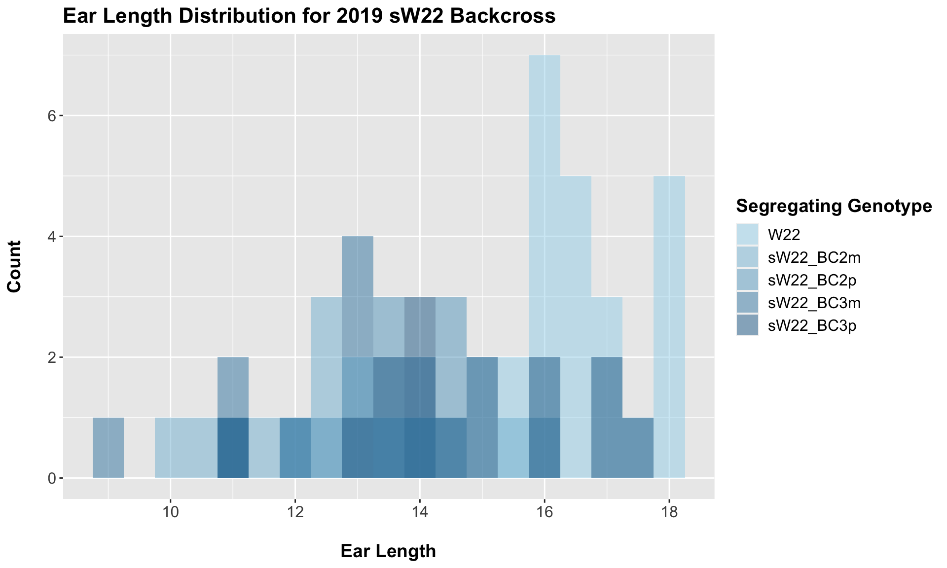
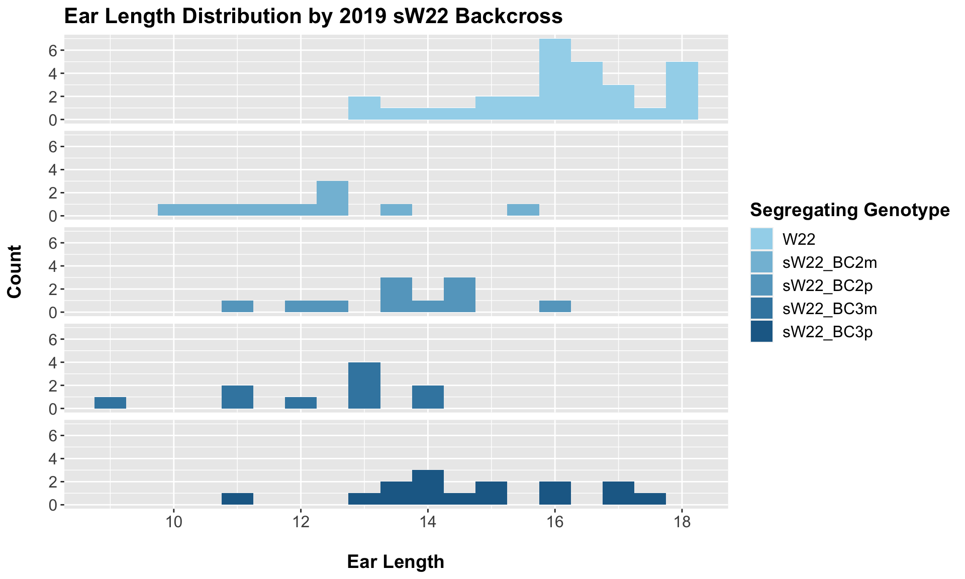
5.1.1 2019 sW22 backcrossed to W22
##
##  Mean, SD, and SE for each genotype
## Seg_Genotype N mean sd se
## 1 W22 30 16.06667 1.430778 0.2612232
## 2 sW22_BC2m 10 12.15000 1.582017 0.5002777
## 3 sW22_BC2p 11 13.59091 1.375103 0.4146092
## 4 sW22_BC3m 10 12.30000 1.567021 0.4955356
## 5 sW22_BC3p 15 14.73333 1.751190 0.4521553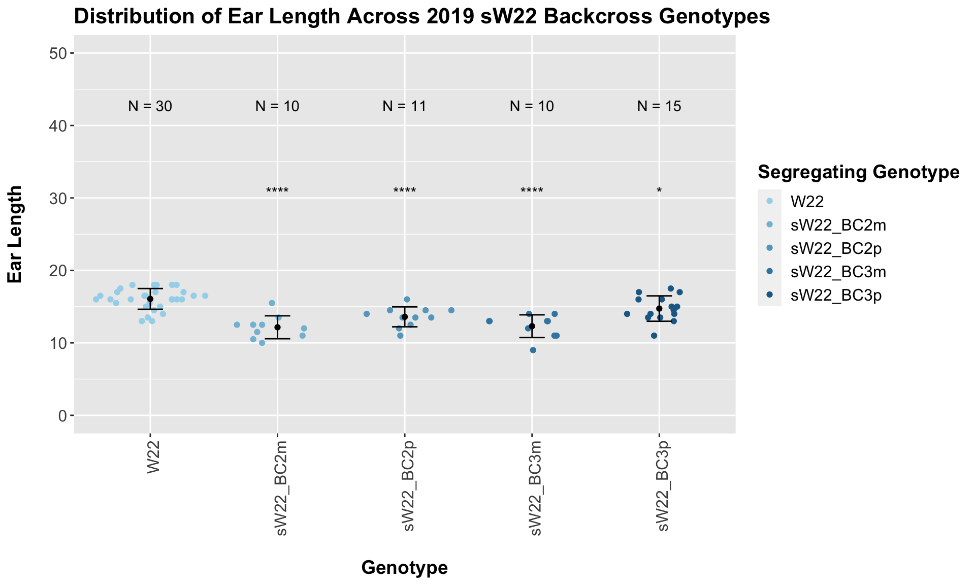
##
## Results of T-test used to obtain significance in the above plot
## # A tibble: 4 x 8
## .y. group1 group2 p p.adj p.format p.signif method
## <chr> <chr> <chr> <dbl> <dbl> <chr> <chr> <chr>
## 1 Ear_Trait W22 sW22_BC2m 0.00000625 0.000025 6.3e-06 **** T-test
## 2 Ear_Trait W22 sW22_BC2p 0.0000764 0.000150 7.6e-05 **** T-test
## 3 Ear_Trait W22 sW22_BC3m 0.00000855 0.000026 8.6e-06 **** T-test
## 4 Ear_Trait W22 sW22_BC3p 0.0176 0.018 0.018 * T-testFrom this, we can see a signficant reduction in ear length among the backcrosses compared to the W22 control. We see a substantial reduction that does improve by backcross generation 3. When we have comparisons between the sick plant being either the maternal or paternal parent, it does seem like the paternal lineage is a bit taller? From our 2020 data, we only had one maternal/paternal comaprison (BC2), and I did not see a noticeable difference between the two.
We may also we separate the data by which field the row was in.
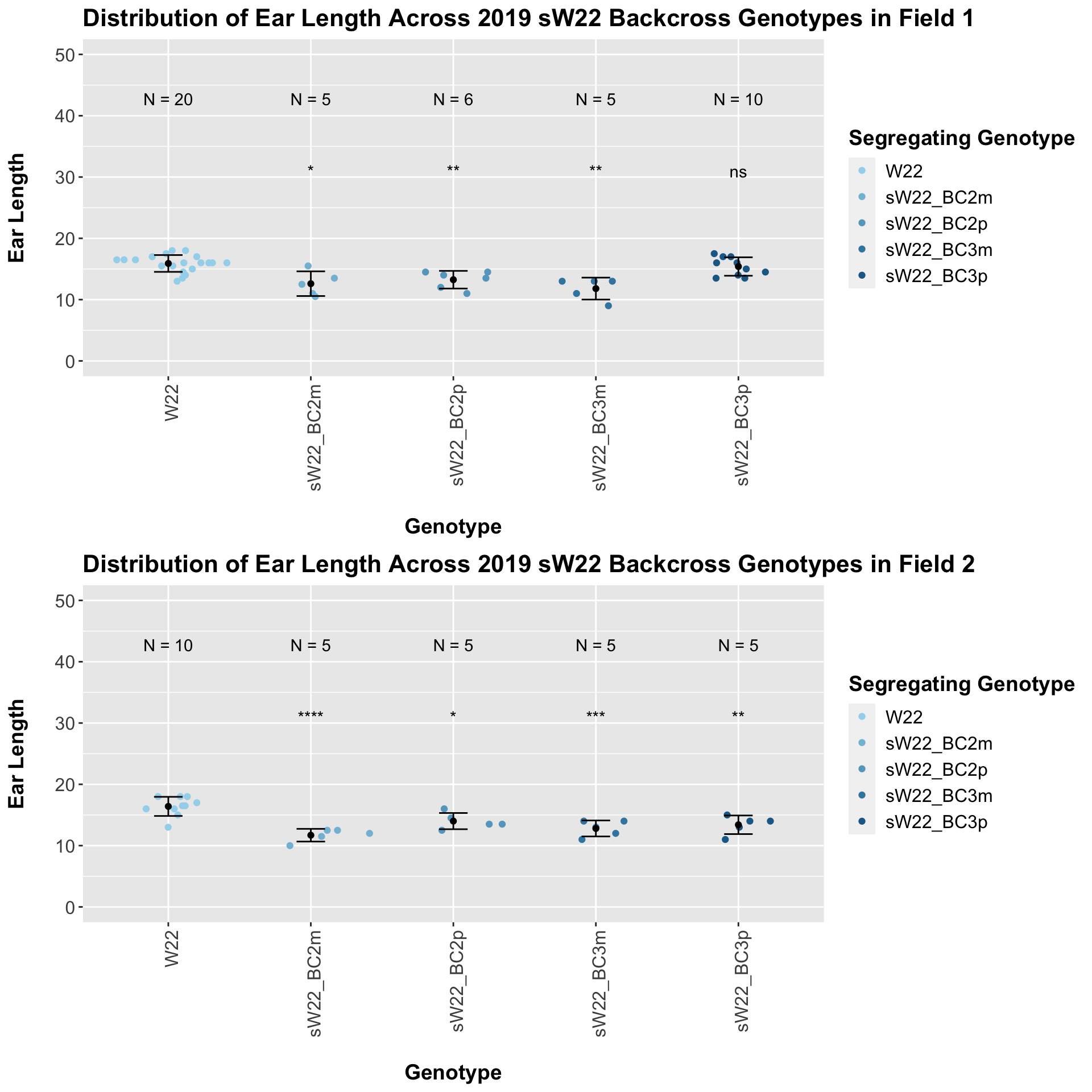
Our results are less significant when we stratify by field, but the trend of a significant reduction that slowly recovers does seem to hold. This may be due to the small number of data points for the backcrosses generations.
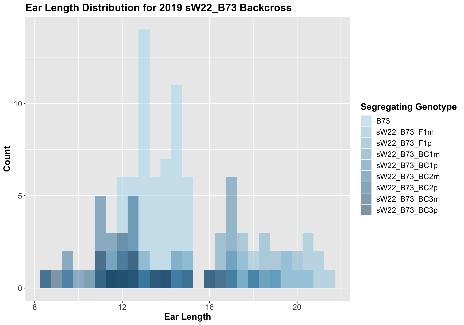
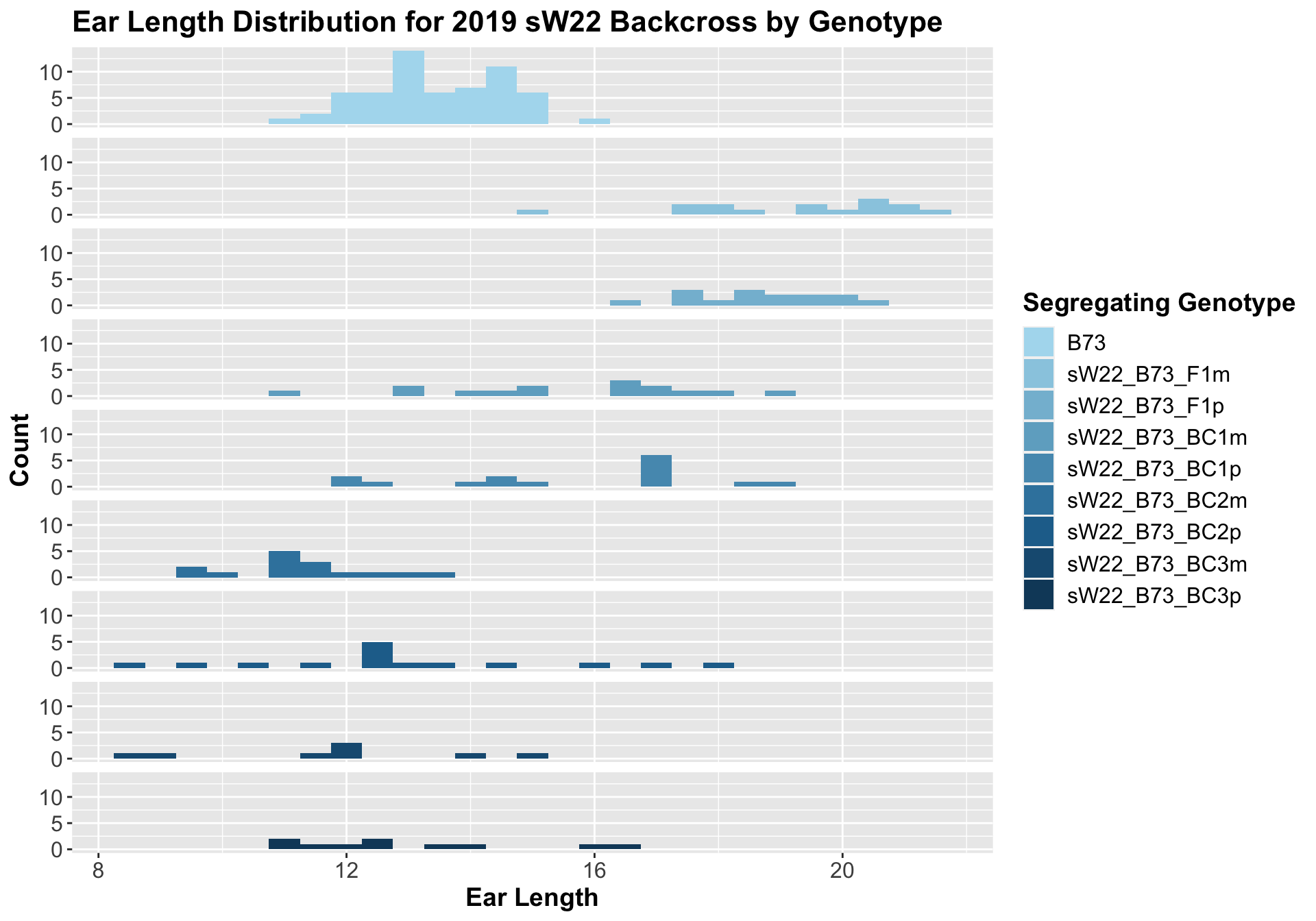
5.1.2 2019 sW22 and W22 backcrossed to B73
##
##  Mean, SD, and SE for each genotype
## Seg_Genotype N mean sd se
## 1 B73 60 13.45833 1.086480 0.1402639
## 2 sW22_B73_F1m 15 19.23333 1.781519 0.4599862
## 3 sW22_B73_F1p 15 18.66667 1.128632 0.2914115
## 4 sW22_B73_BC1m 15 15.56667 2.178357 0.5624493
## 5 sW22_B73_BC1p 15 15.60000 2.277216 0.5879747
## 6 sW22_B73_BC2m 15 11.30000 1.146423 0.2960051
## 7 sW22_B73_BC2p 15 12.96667 2.601282 0.6716481
## 8 sW22_B73_BC3m 8 11.75000 2.203893 0.7791937
## 9 sW22_B73_BC3p 10 13.05000 1.950071 0.6166667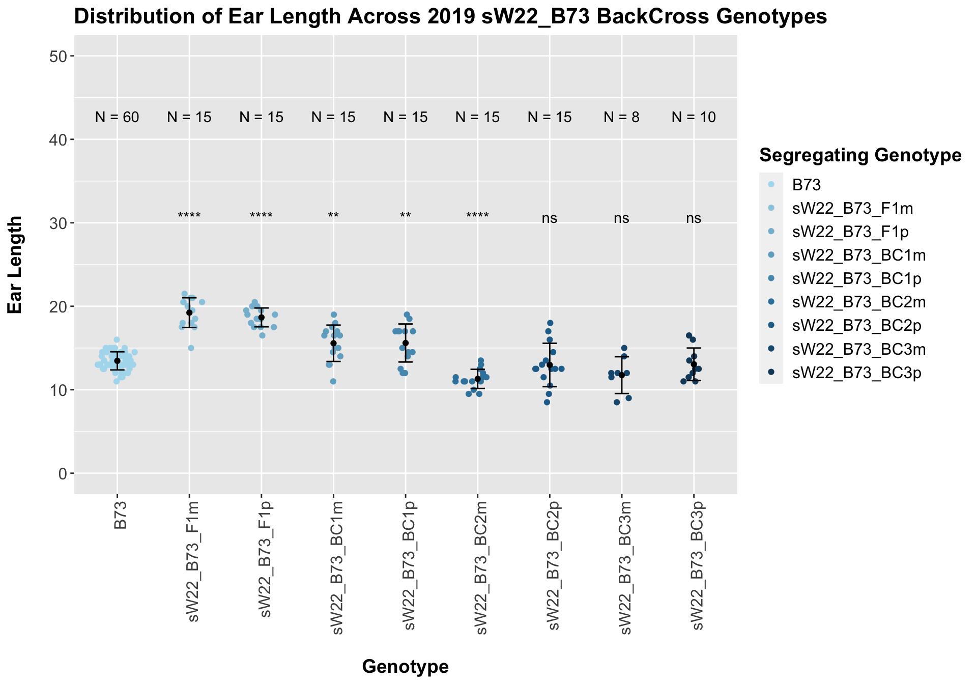
## # A tibble: 8 x 8
##   .y.       group1 group2               p    p.adj p.format p.signif method
##   <chr>     <chr>  <chr>            <dbl>    <dbl> <chr>    <chr>    <chr>
## 1 Ear_Trait B73    sW22_B73_F1m  1.24e- 9 8.70e- 9 1.2e-09  ****     T-test
## 2 Ear_Trait B73    sW22_B73_F1p  2.78e-13 2.20e-12 2.8e-13  ****     T-test
## 3 Ear_Trait B73    sW22_B73_BC1m 2.26e- 3 1.10e- 2 0.0023   **       T-test
## 4 Ear_Trait B73    sW22_B73_BC1p 2.79e- 3 1.10e- 2 0.0028   **       T-test
## 5 Ear_Trait B73    sW22_B73_BC2m 1.69e- 6 1.00e- 5 1.7e-06  ****     T-test
## 6 Ear_Trait B73    sW22_B73_BC2p 4.84e- 1 9.70e- 1 0.4845   ns       T-test
## 7 Ear_Trait B73    sW22_B73_BC3m 6.54e- 2 2.00e- 1 0.0654   ns       T-test
## 8 Ear_Trait B73    sW22_B73_BC3p 5.33e- 1 9.70e- 1 0.5331   ns       T-test
Here, we see a significant increase in ear length for the initial F1s that slowly decline until there is no significant difference between the backcrosses and the B73 data.
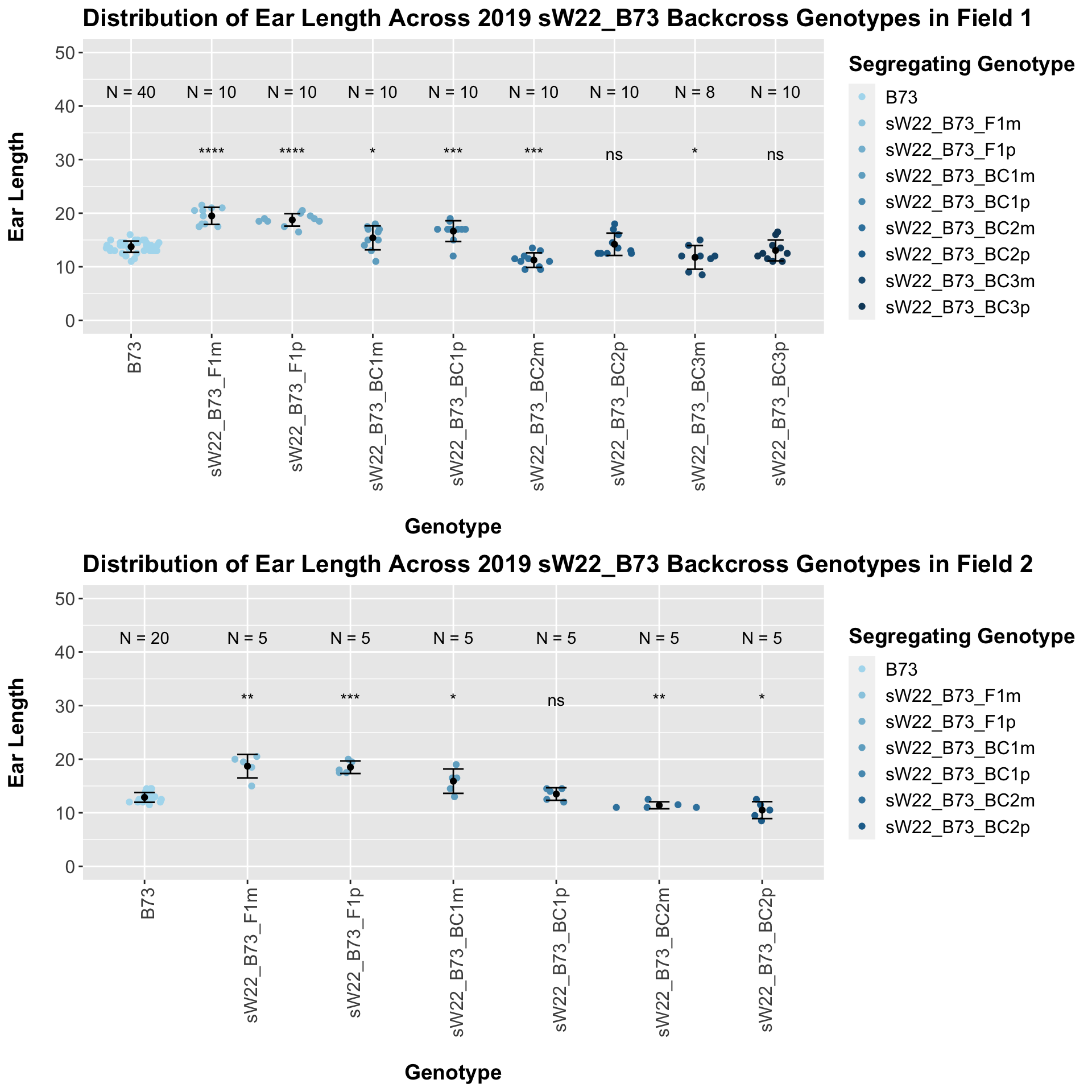
If we separate by field, we see that the trend does hold, but it is less significant than the combined data. We can compare the height data across the W22 backcrossed to B73 rows to look at this set of controls.
##
##  Mean, SD, and SE for each genotype
## Seg_Genotype N mean sd se
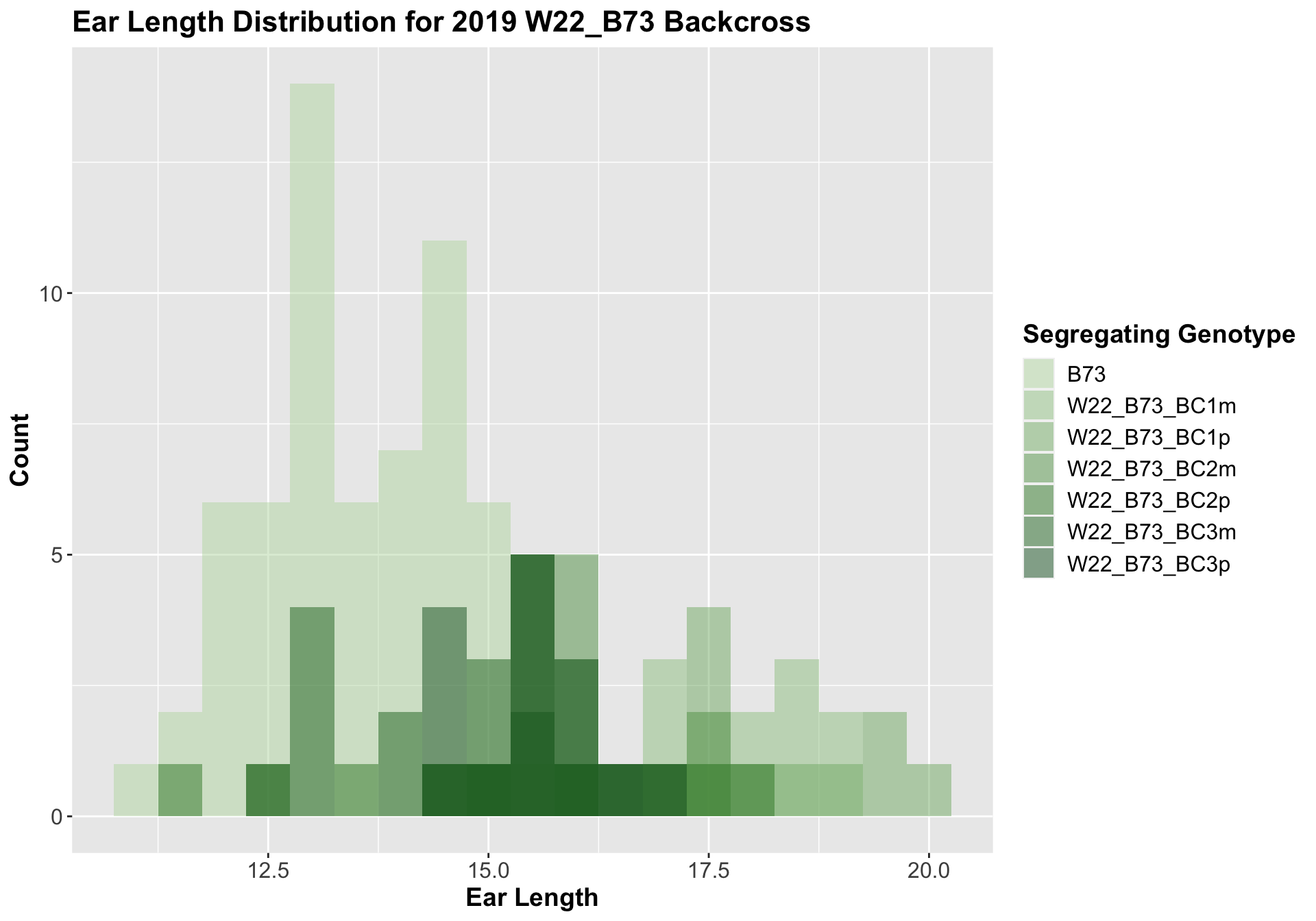
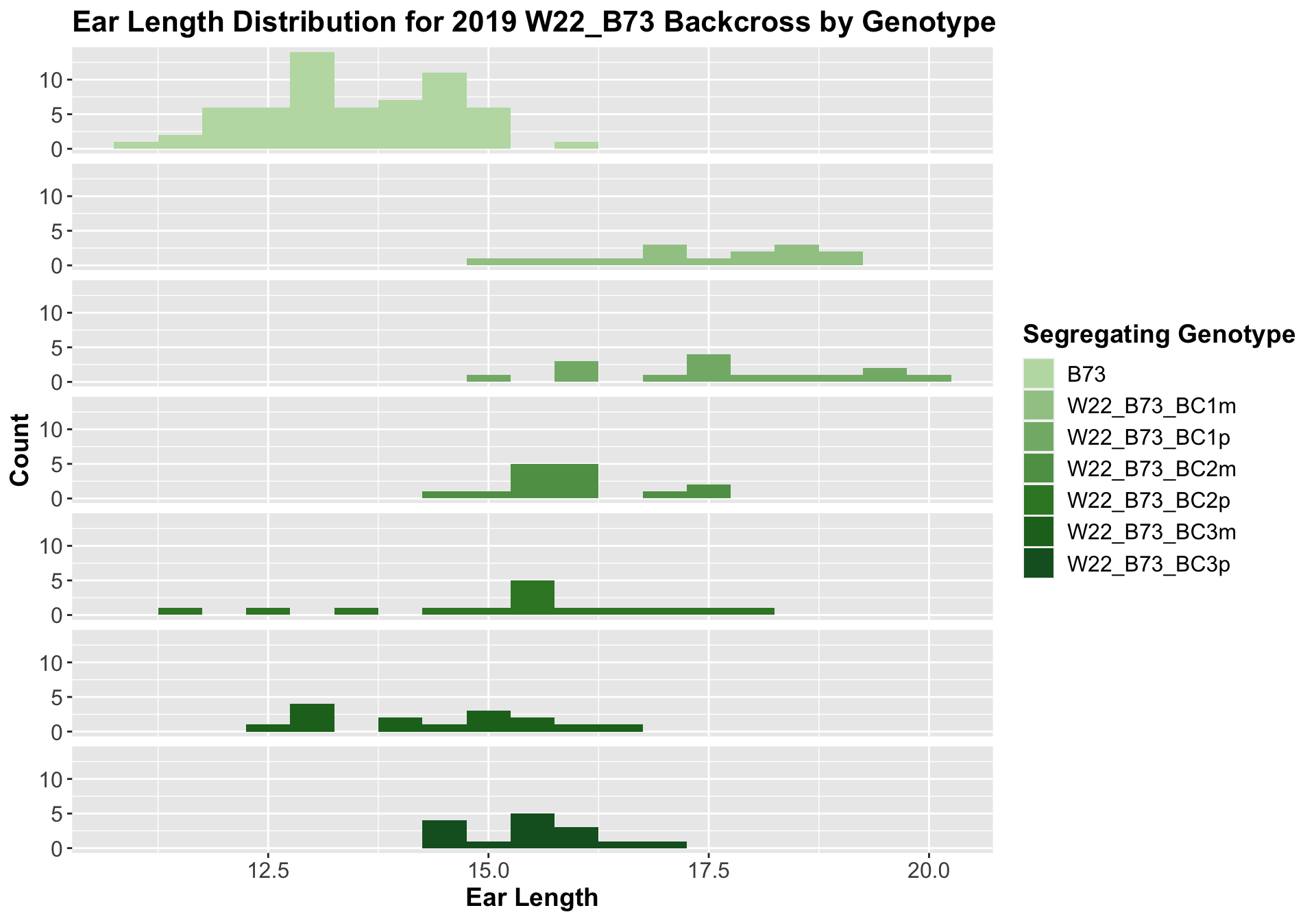
## 1 B73 60 13.45833 1.0864796 0.1402639
## 2 W22_B73_BC1m 15 17.40000 1.2564121 0.3244042
## 3 W22_B73_BC1p 15 17.63333 1.4816336 0.3825561
## 4 W22_B73_BC2m 15 15.93333 0.8423324 0.2174893
## 5 W22_B73_BC2p 15 15.30000 1.7606817 0.4546061
## 6 W22_B73_BC3m 15 14.36667 1.2601965 0.3253813
## 7 W22_B73_BC3p 15 15.46667 0.7668737 0.1980059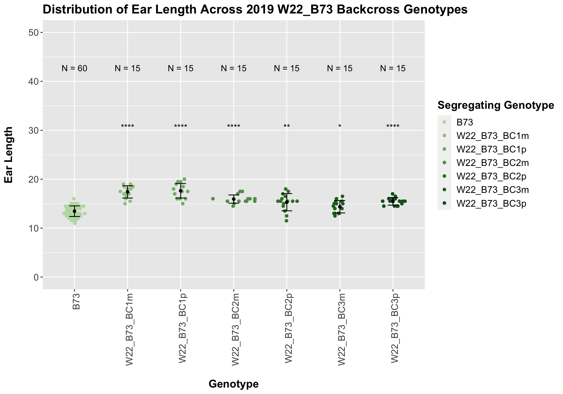
## # A tibble: 6 x 8
##   .y.       group1 group2              p        p.adj p.format p.signif method
##   <chr>     <chr>  <chr>           <dbl>        <dbl> <chr>    <chr>    <chr>
## 1 Ear_Trait B73    W22_B73_BC1m 6.33e-10 0.0000000032 6.3e-10  ****     T-test
## 2 Ear_Trait B73    W22_B73_BC1p 6.34e- 9 0.000000019  6.3e-09  ****     T-test
## 3 Ear_Trait B73    W22_B73_BC2m 3.72e-10 0.0000000022 3.7e-10  ****     T-test
## 4 Ear_Trait B73    W22_B73_BC2p 1.26e- 3 0.0025       0.0013   **       T-test
## 5 Ear_Trait B73    W22_B73_BC3m 1.87e- 2 0.019        0.0187   *        T-test
## 6 Ear_Trait B73    W22_B73_BC3p 3.24e- 9 0.000000013  3.2e-09  ****     T-test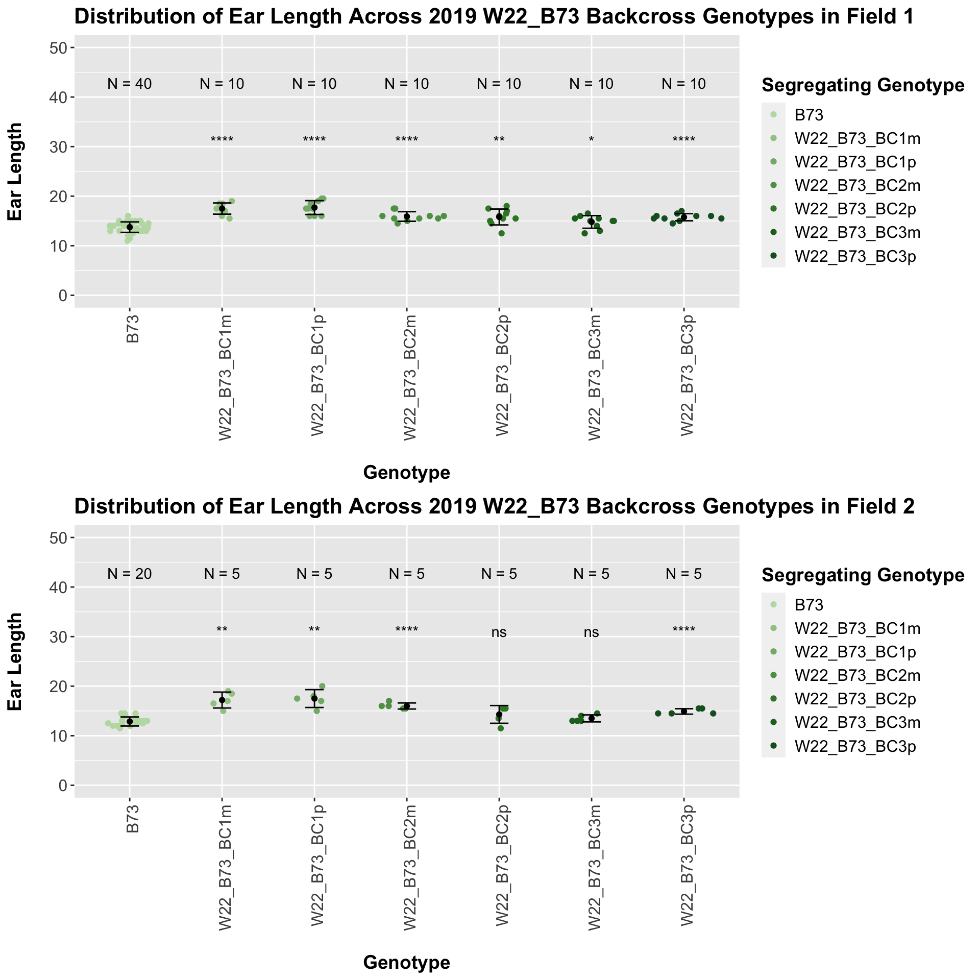
Once again, we see an initial increase in ear length among our backcrosses that slowly declines. This pattern holds if we separate by field, but, once again, the difference between the backcross and the B73 line becomes marginal.
We may also compare the distribution for sW22_B73 backcrosses to W22_B73 backcrosses and each generation compares across these two sets. Note: when looking at these plots, just be aware that the genotypes don't align perfectly across backcrosses because we don't have a few crosses for the W22_B73 genotypes.
When we specifically compare the height between sW22 and W22 backcrossed to B73 at each generation, we see a significant reduction in height of the sW22 backcross against the W22 backcross. If we stratify this data by field, we see that this continues to remain significant.
5.1.3 2019 sW22 and W22 backcrossed to Mo17
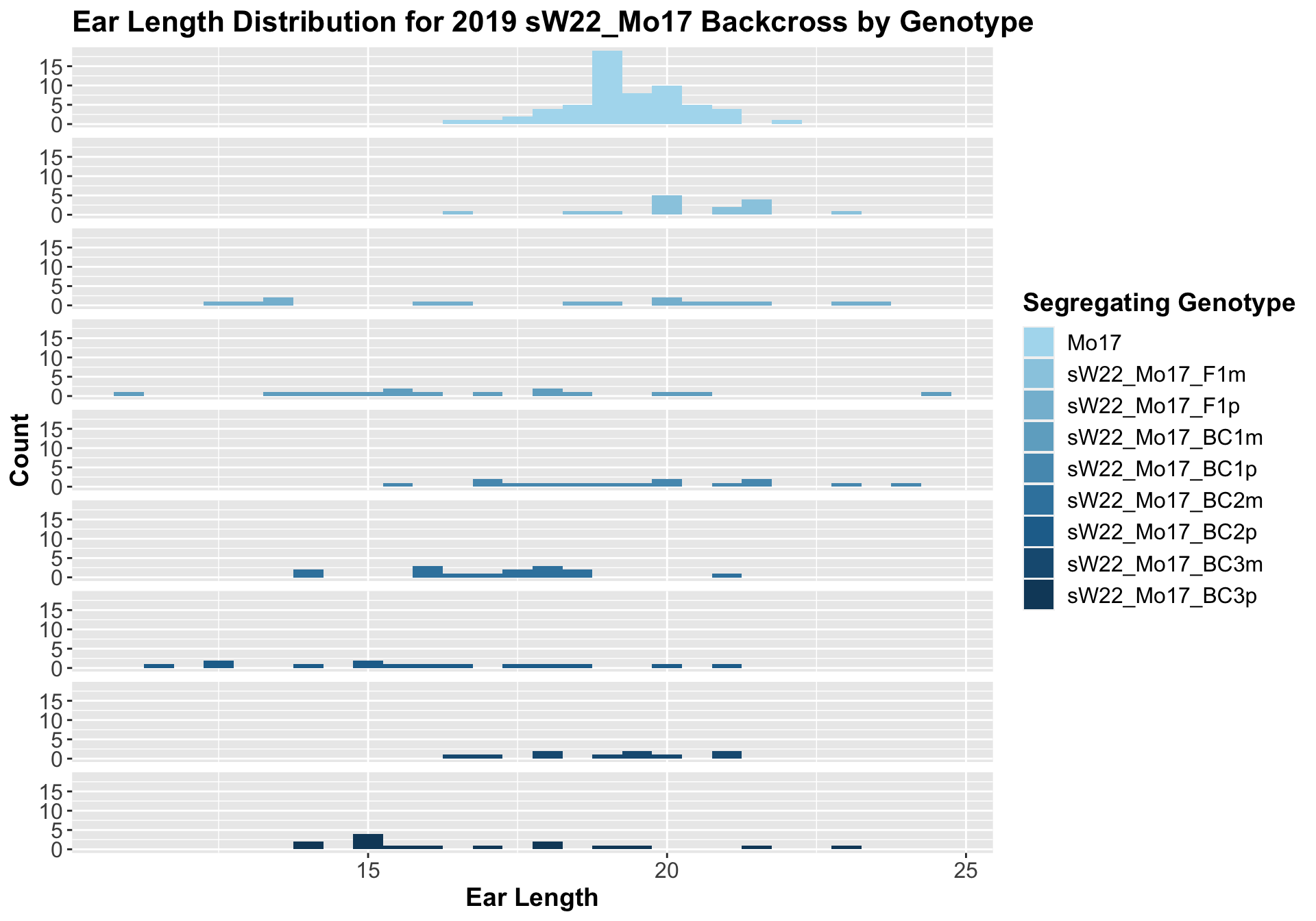
##
##  Mean, SD, and SE for each genotype
## Seg_Genotype N mean sd se
## 1 Mo17 60 19.30833 1.029611 0.1329222
## 2 sW22_Mo17_F1m 15 20.33333 1.554563 0.4013865
## 3 sW22_Mo17_F1p 15 18.13333 3.719959 0.9604893
## 4 sW22_Mo17_BC1m 15 16.76667 3.315907 0.8561635
## 5 sW22_Mo17_BC1p 15 19.53333 2.378975 0.6142488
## 6 sW22_Mo17_BC2m 15 17.10000 1.794834 0.4634241
## 7 sW22_Mo17_BC2p 14 15.96429 2.838365 0.7585851
## 8 sW22_Mo17_BC3m 10 18.95000 1.553669 0.4913134
## 9 sW22_Mo17_BC3p 15 17.03333 2.748160 0.7095717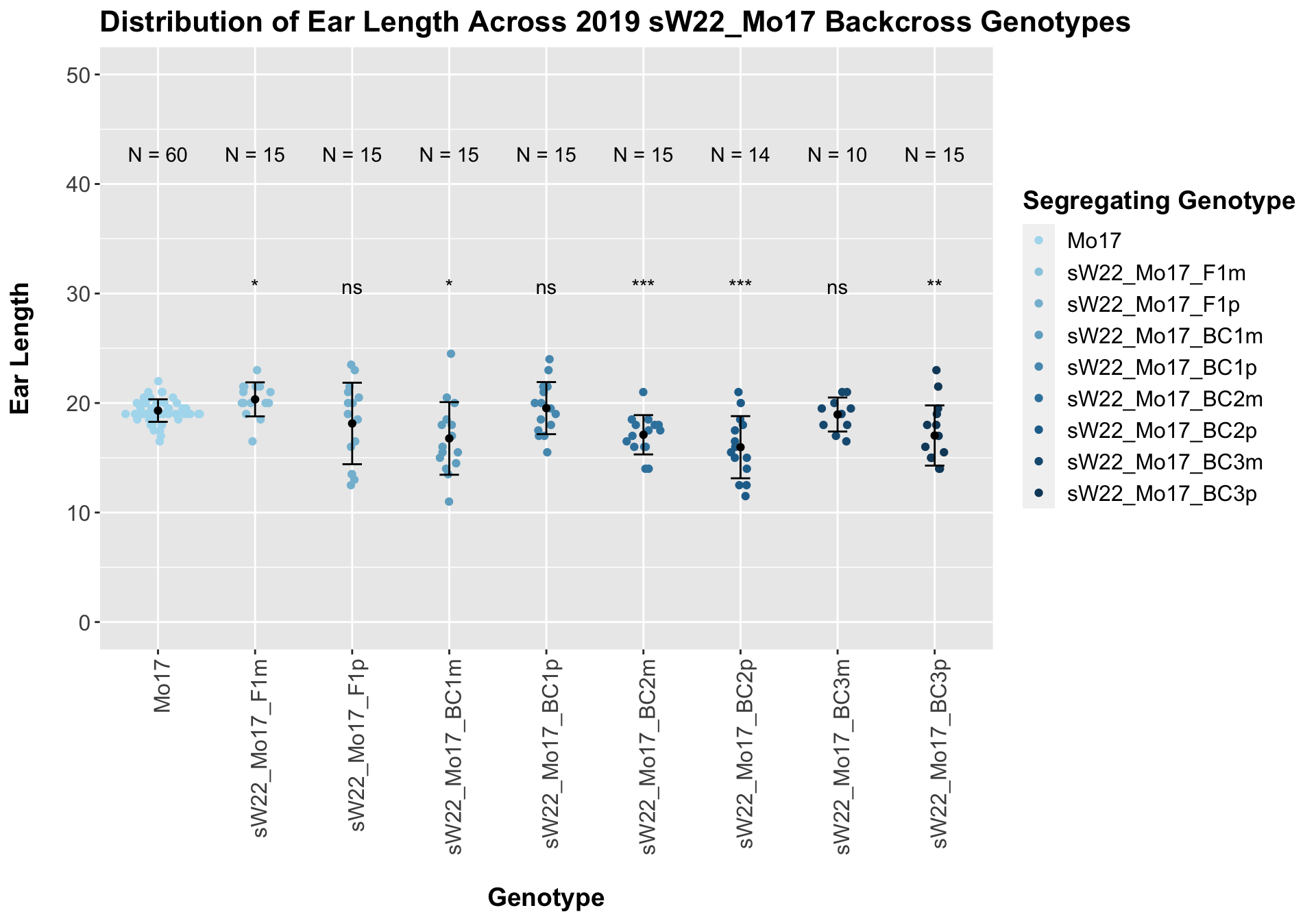
## # A tibble: 8 x 8
##   .y.       group1 group2                p  p.adj p.format p.signif method
##   <chr>     <chr>  <chr>             <dbl>  <dbl> <chr>    <chr>    <chr>
## 1 Ear_Trait Mo17   sW22_Mo17_F1m  0.0266   0.11   0.02665  *        T-test
## 2 Ear_Trait Mo17   sW22_Mo17_F1p  0.245    0.73   0.24492  ns       T-test
## 3 Ear_Trait Mo17   sW22_Mo17_BC1m 0.0105   0.052  0.01046  *        T-test
## 4 Ear_Trait Mo17   sW22_Mo17_BC1p 0.725    0.99   0.72521  ns       T-test
## 5 Ear_Trait Mo17   sW22_Mo17_BC2m 0.000291 0.0023 0.00029  ***      T-test
## 6 Ear_Trait Mo17   sW22_Mo17_BC2p 0.000697 0.0049 0.00070  ***      T-test
## 7 Ear_Trait Mo17   sW22_Mo17_BC3m 0.497    0.99   0.49694  ns       T-test
## 8 Ear_Trait Mo17   sW22_Mo17_BC3p 0.00659  0.04   0.00659  **       T-test
Here, we don't see a very strong correlation between sW22 backcrossed to Mo17. Occassionally, the backcrosses have a shorter ear length, but it is not consistently significant.
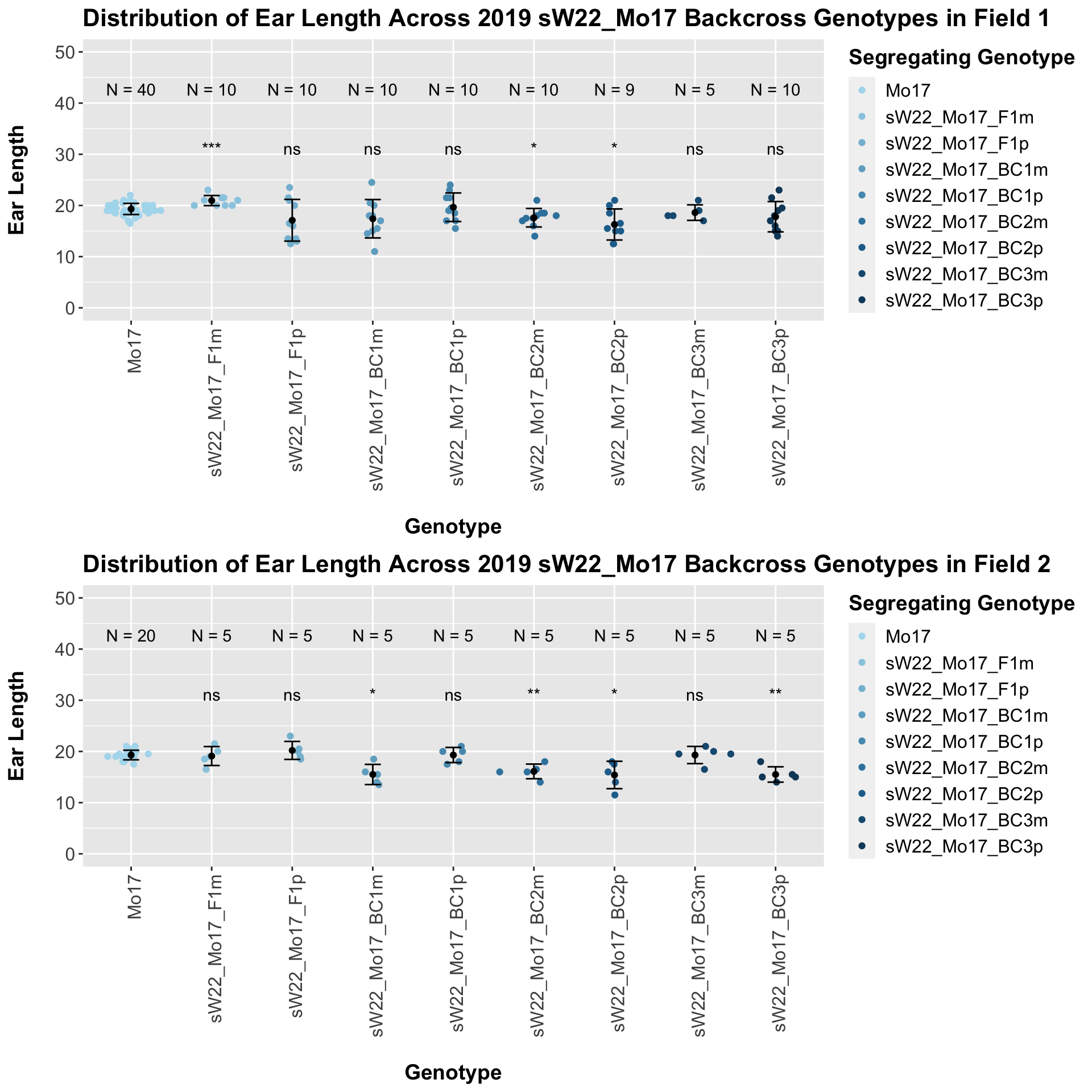
The field data is very similar to the data in aggregate. We often see an insignificant or marginal change in ear length.
We can compare the height data across the W22 backcrossed to Mo17 rows
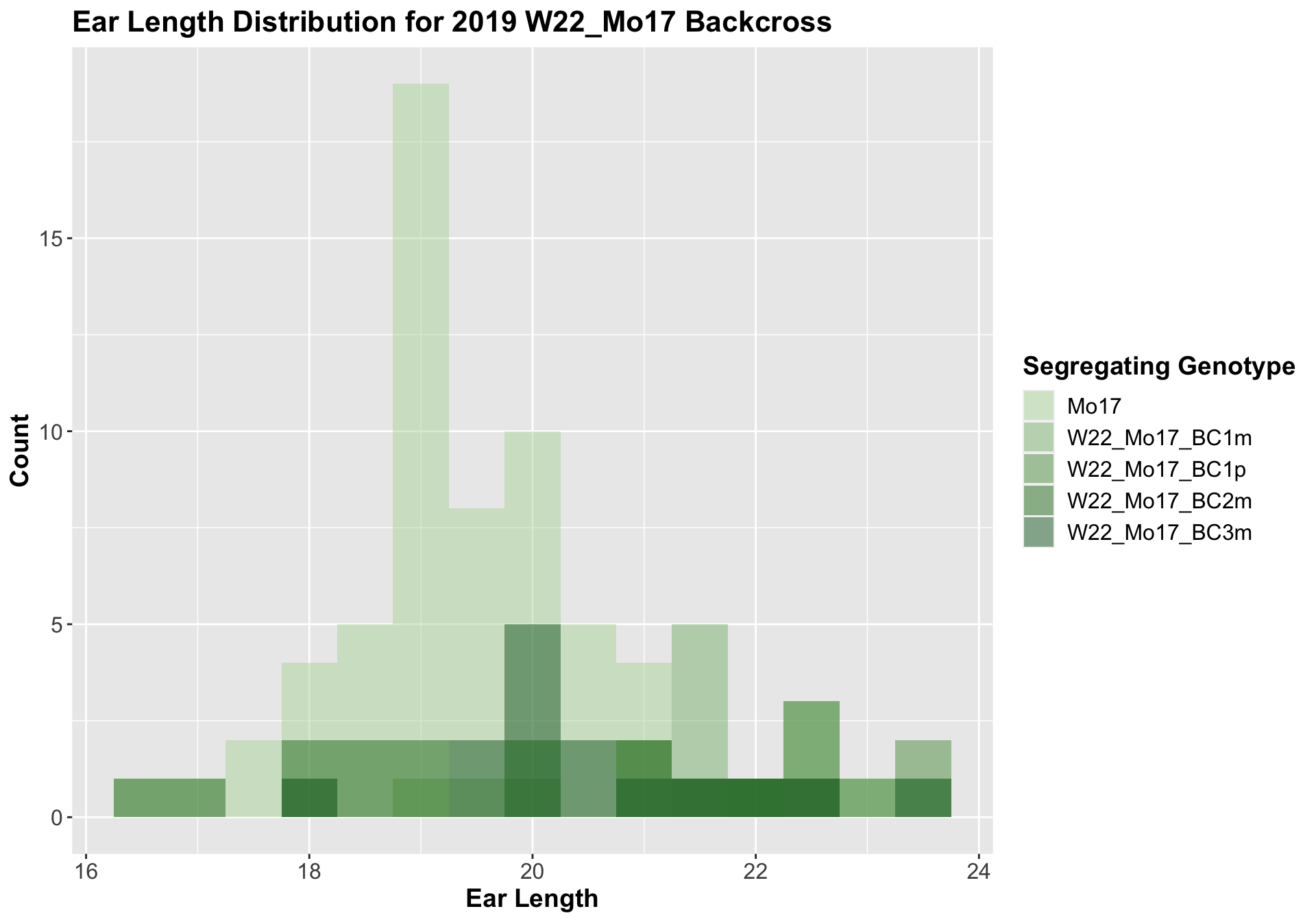
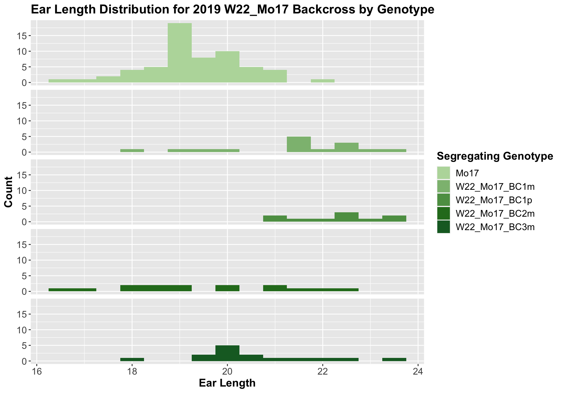
##
##  Mean, SD, and SE for each genotype
## Seg_Genotype N mean sd se
## 1 Mo17 60 19.30833 1.0296110 0.1329222
## 2 W22_Mo17_BC1m 15 21.33333 1.5545632 0.4013865
## 3 W22_Mo17_BC1p 10 22.30000 0.9189366 0.2905933
## 4 W22_Mo17_BC2m 15 19.50000 1.8224787 0.4705620
## 5 W22_Mo17_BC3m 15 20.56667 1.3610220 0.3514144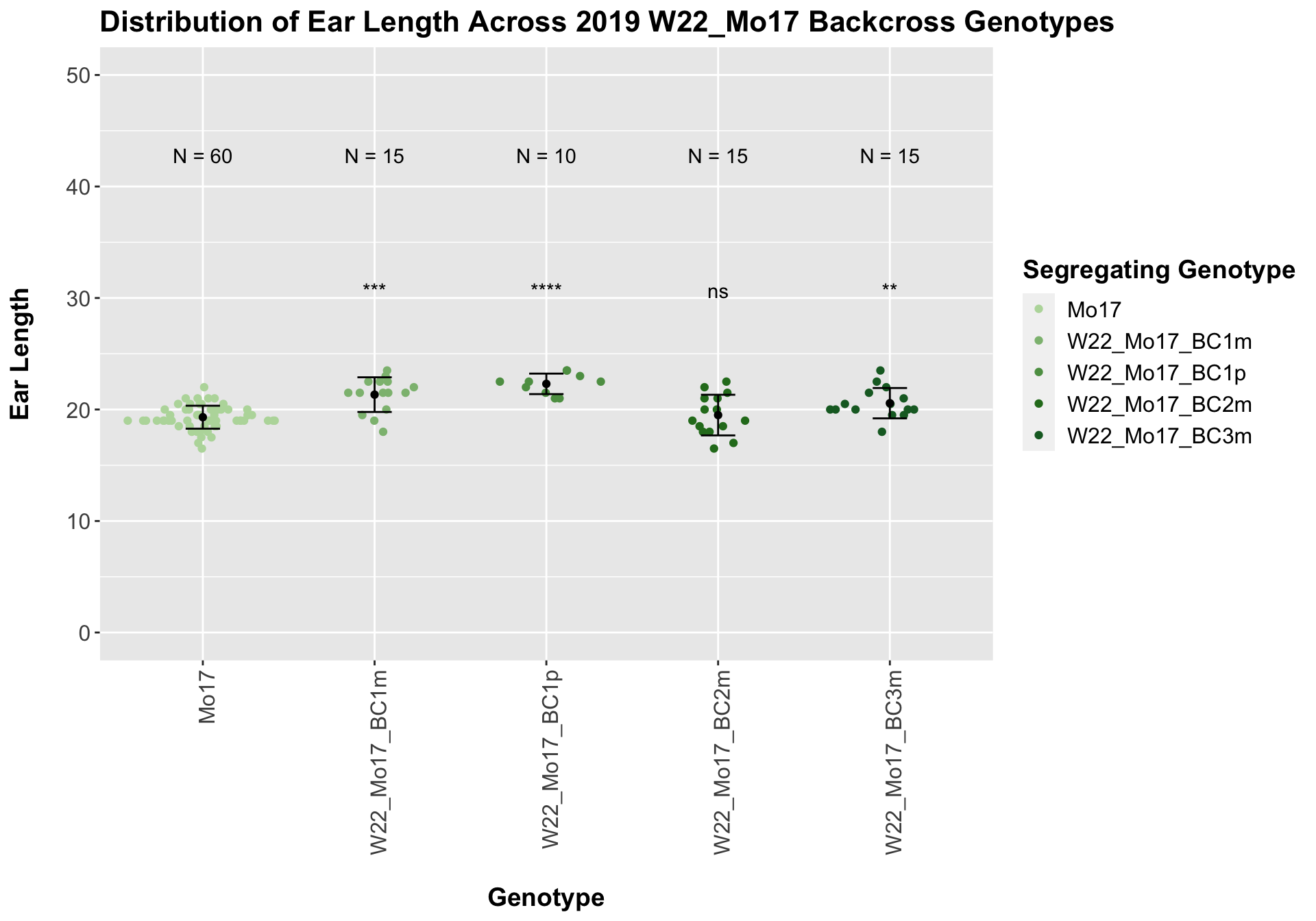
## # A tibble: 4 x 8
##   .y.       group1 group2                  p     p.adj p.format p.signif method
##   <chr>     <chr>  <chr>               <dbl>     <dbl> <chr>    <chr>    <chr>
## 1 Ear_Trait Mo17   W22_Mo17_BC1m 0.000166    0.0005    0.00017  ***      T-test
## 2 Ear_Trait Mo17   W22_Mo17_BC1p 0.000000367 0.0000015 3.7e-07  ****     T-test
## 3 Ear_Trait Mo17   W22_Mo17_BC2m 0.700       0.7       0.70015  ns       T-test
## 4 Ear_Trait Mo17   W22_Mo17_BC3m 0.00353     0.0071    0.00353  **       T-test
We see an increase in ear length followed by a decline at each backcross. Once, again, we separate the data by field, to see whether the trend is the same.
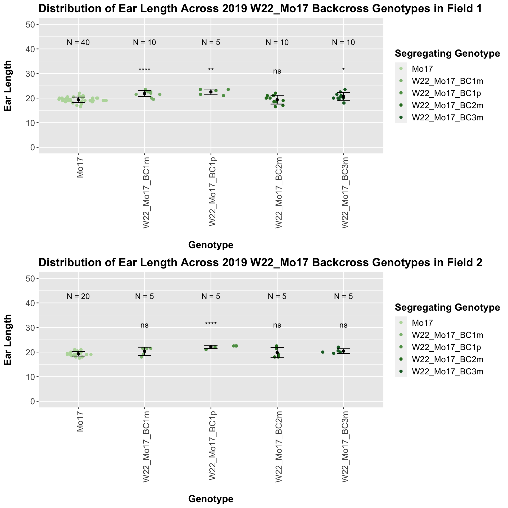
The trend holds, but it does not seem to be as significant.
We now compare the distribution for sW22_Mo17 backcrosses to W22_Mo17 backcrosses and how each generaiton compares across these two sets. Note: when looking at these plots, just be aware that the genotypes don't align perfectly across backcrosses because we don't have a few crosses for the W22_Mo17 genotypes.
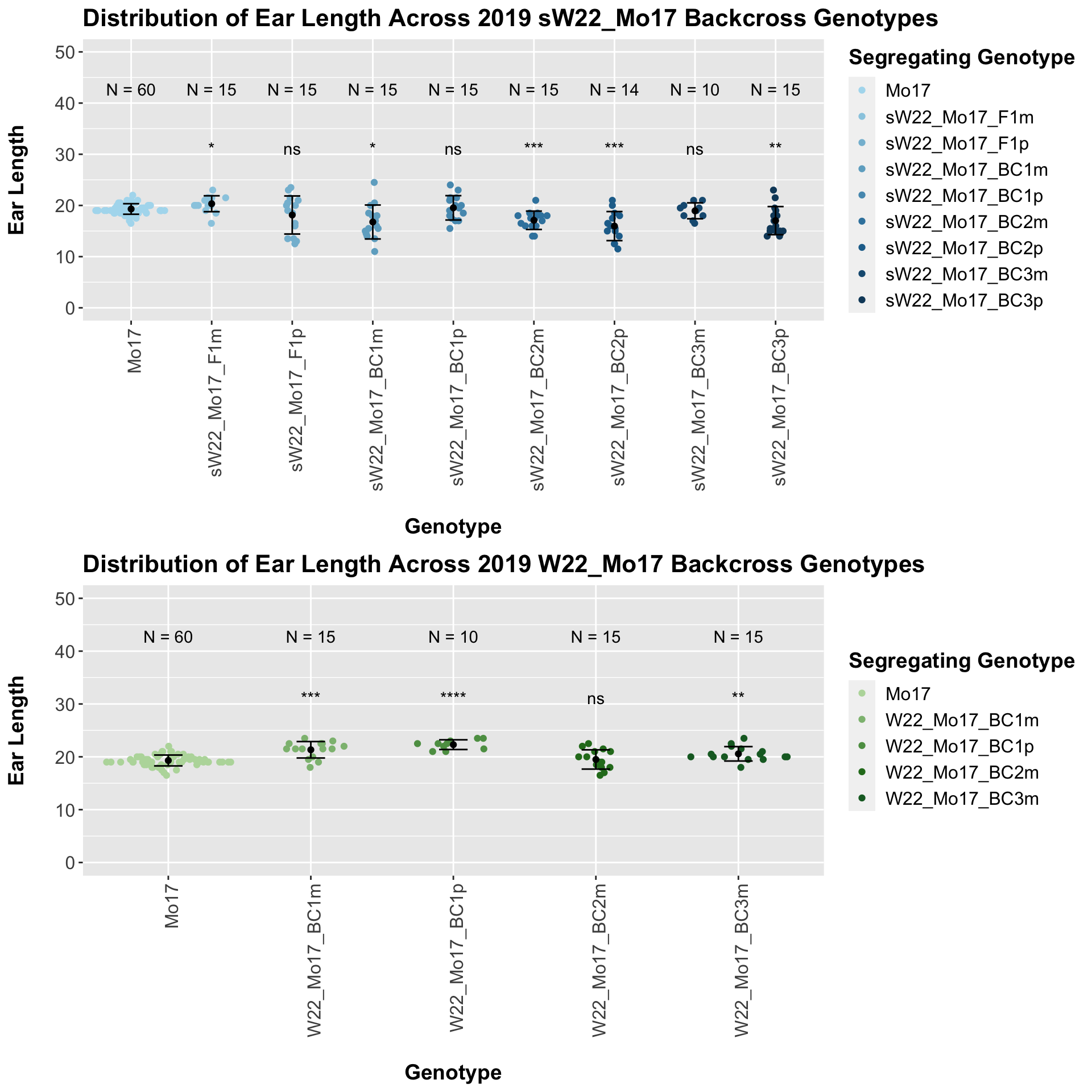
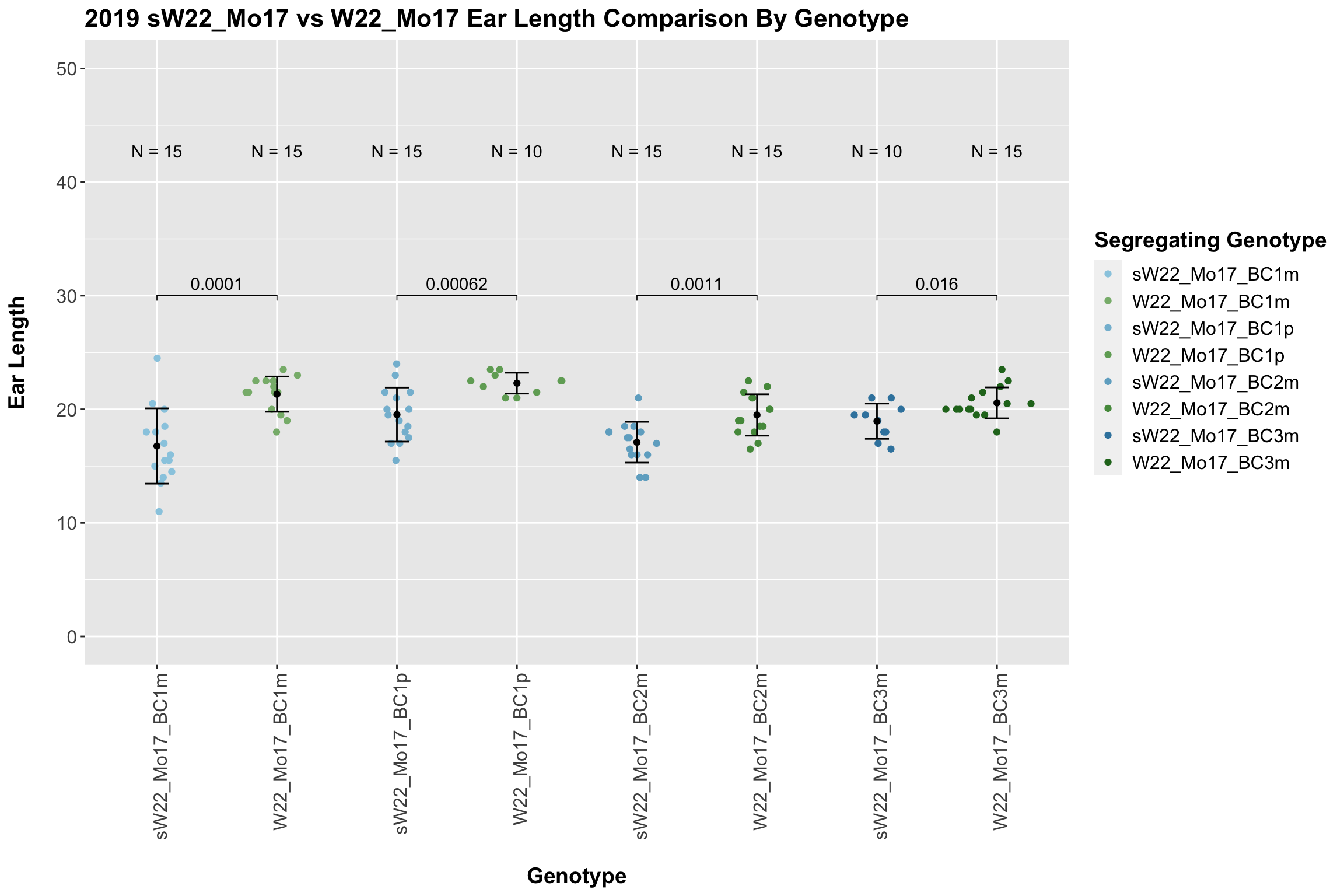
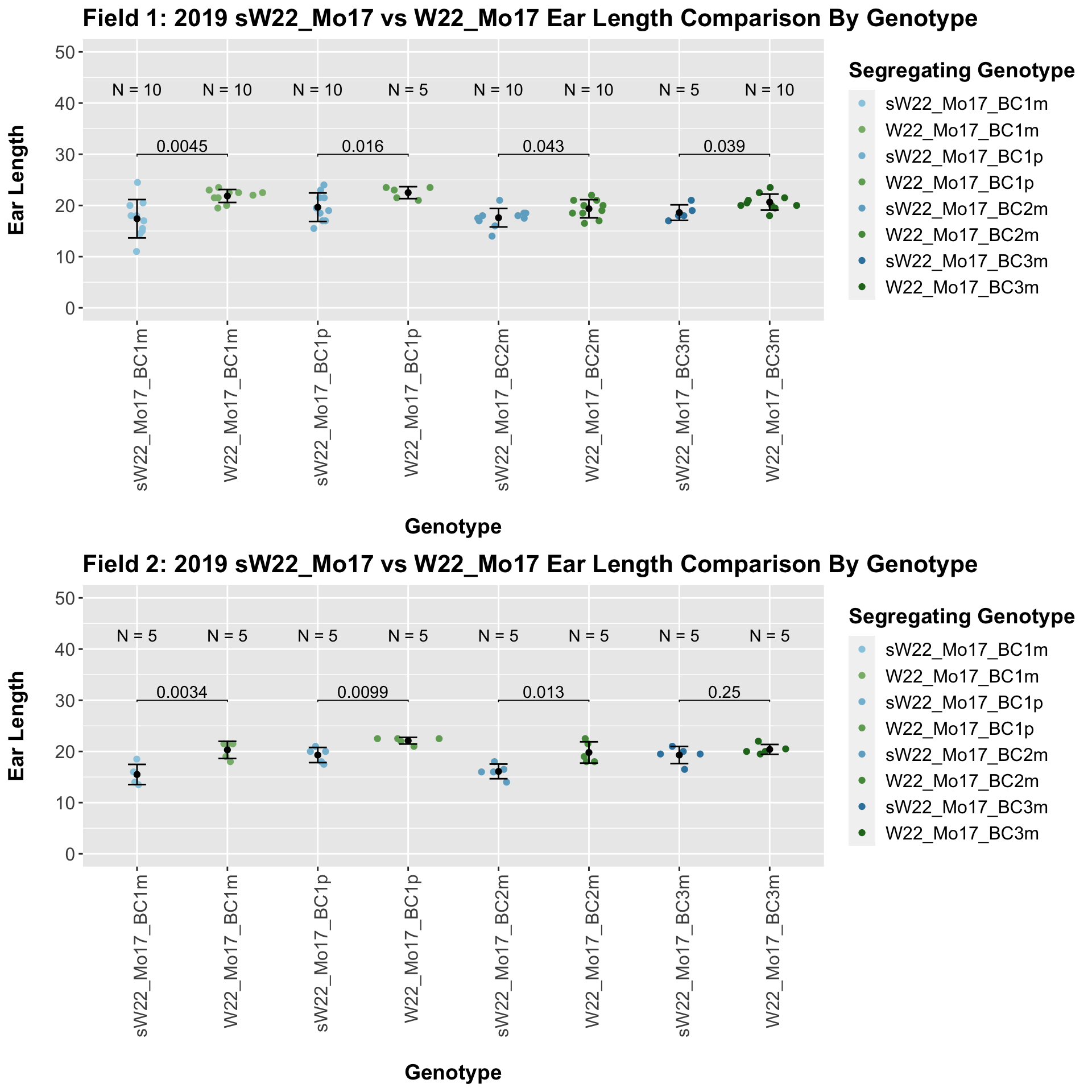
We find that there is a significant reduction in ear length for the sW22_Mo17 backcrosses compared to the W22_Mo17 backcrosses.
We may also compare the distribution for all sW22 backcrosses (crossed to W22, B73, and Mo17 respectively). Note: when looking at these plots, just be aware that the genotypes don't align perfectly across backcrosses so be sure to check the x-axis.

5.1.4 2019 ANOVA for Ear Length
We now want to test whether (1) ear length is impacted by the sex of the sick parent and (2) the means across each backcross generation change #### . We also transformed the categorical genotype values (F1,BC1,BC2,BC3,BC4,BC5) to numerical values (0,1,2,3,4,5).
We start by fitting a series of linear models:
- mod_full_int: Ear_Length (Numerical) ~ Field (Cateogrical) + Genotype (Numerical) + Sick_Sex (Categorical) + Genotype*Sick_Sex
- mod_full: Ear_Length (Numerical) ~ Field (Categorical) + Genotype (Numerical) + Sick_Sex (Categorical)
- mod_geno: Ear_Length (Numerical) ~ Field (Cateogrical) + Genotype (Numerical)
- mod_sex: Ear_Length (Numerical) ~ Field + Sick_Sex (Categorical)
We can then compare the fit of these models to our data using an ANOVA to test whether the more complex model (mod_full) is significantly better at capturing our height data than either of our simpler models. This will tell us whether incorporating sex/genotype significantly improves our model.
We can summarize the results of this across each set of genotypes. The significance codes are as follows:
- '***' - between 0 and 0.001
- '**' - between 0.001 and 0.01
- '*' - between 0.01 and 0.05
- '.' - between 0.05 and 0.1
- ' ' - between 0.1 and 1
##    Geno_Set  Sex_PValue Sex_Signif Genotype_PValue Genotype_Signif
## 1  sW22_W22 0.000242345        ***    1.622735e-01
## 2  sW22_B73 0.153716290               1.858024e-24             ***
## 3 sW22_Mo17 0.385178464               1.503581e-02               *
## 4   W22_B73 0.397966059               1.864605e-11             ***
## 5  W22_Mo17 0.021112068          *    1.985123e-01
##   Sex_Geno_Int_PValue Sex_Geno_Int_Signif
## 1          0.32971698
## 2          0.02338886                   *
## 3          0.74829786
## 4          0.19946173
## 5                  NA